Spatiotemporal Downscaling Model for Solar Irradiance Forecast Using Nearest-Neighbor Random Forest and Gaussian Process

Abstract

Accurate solar photovoltaic (PV) capacity estimation requires high-resolution, site-specific solar irradiance data to account for localized variability. However, global datasets, such as the National Solar Radiation Database (NSRDB), provide regional averages that fail to capture the fine-scale fluctuations critical for large-scale grid integration. This limitation is particularly relevant in the context of increasing distributed energy resources (DERs) penetration, such as rooftop PV. Additionally, it is critical to the implementation of the U.S. Federal Energy Regulatory Commission (FERC) Order 2222, which facilitates DER participation in U.S. bulk power markets. To address this challenge, this study evaluates Nearest-Neighbor Random Forest (NNRF) and Nearest-Neighbor Gaussian Process (NNGP) models for spatiotemporal downscaling of global solar irradiance data. By leveraging historical irradiance and meteorological data, these models incorporate spatial, temporal, and feature-based correlations to enhance local irradiance predictions. The NNRF model, a machine-learning approach, prioritizes computational efficiency and predictive accuracy, while the NNGP model offers a level of interpretability and prediction uncertainty by numerically quantifying correlations and dependencies in the data. Model validation was conducted using day-ahead predictions. The results showed that the average Goodness of Fit (GoF) of the NNRF model of 90.61% across all eight sites outperformed the GoF of the NNGP of 85.88%. Additionally, the computational speed of NNRF was 2.5 times faster than the NNGP. Finally, the NNGP displayed polynomial scaling while the NNRF scaled linearly with increasing number of nearest neighbors. Additional validation of the model on five sites in Puerto Rico further confirmed the superiority of the NNRF model over the NNGP model. These findings highlight the robustness and computational efficiency of NNRF for large-scale solar irradiance downscaling, making it a strong candidate for improving PV capacity estimation and real-time electricity market integration for DERs.

1. Introduction

The global push for decarbonization has driven regulatory developments such as the U.S. Federal Energy Regulatory Commission (FERC) Order 2222 [1], which enables the participation of distributed energy resources (DERs), including rooftop solar photovoltaic (PV) systems, in wholesale electricity markets. This regulatory shift is accelerating the integration of renewable energy resources and reshaping both power system operations and market dynamics [2]. However, integrating variable renewable energy resources (VREs) like solar PV presents significant challenges for grid stability, reliability, and dispatch [3]. Unlike conventional generators, VREs exhibit volatile output due to rapid fluctuations in cloud cover, humidity, and other localized weather conditions. As a result, accurate and high-resolution solar irradiance forecasting is essential for managing DERs effectively within the power grid. However, existing global irradiance models typically operate at coarse spatial and temporal resolutions, limiting their utility for site-specific forecasting and real-time grid operations.

Advances in power electronic converter (PEC) technology, such as improved dynamic models [4] and virtual inertia solutions [5], address some stability concerns. However, accurate solar PV forecasting remains a critical challenge for grid operators and market participants. Existing approaches for solar PV forecasting primarily rely on numerical weather prediction (NWP) models [6,7], statistical methods and machine-learning techniques [8,9,10,11], deep learning algorithms [12,13], and hybrid approaches [9,14,15]. Some studies incorporate probabilistic methods to quantify uncertainty [16,17,18], while others consider the spatial influence of neighboring sites on a target location [12,19]. Although these methods have demonstrated success, many rely on an implicit assumption that global solar irradiance datasets provide accurate site-specific representations. This assumption introduces inaccuracies because global datasets, such as those from the National Solar Radiation Database (NSRDB) [20], provide irradiance values averaged over large spatial scales (e.g., 4 km × 4 km), which fail to capture fine-grained local variability at individual DERs.

A key challenge in solar PV forecasting is the need for high-resolution, site-specific solar irradiance data. Current datasets from sources like NSRDB and Open Meteo [21] cover broad spatial regions, with some reaching resolutions as coarse as 11 km × 11 km. This leads to approximation errors that can undermine accurate capacity estimation and power system operations such as dispatch and balancing. While the ideal solution would involve deploying weather stations at every prospective PV site to obtain direct irradiance measurements, this approach is impractical due to cost, maintenance, and logistical constraints. Furthermore, it would be infeasible for forecasting irradiance at prospective solar PV sites where physical measurements are not yet available. Therefore, there is a pressing need for advanced downscaling techniques that can transform coarse global irradiance data into high-resolution, site-specific estimates suitable for real-time market operations and DER integration.

By leveraging historical data on both global and local solar irradiance measurements, models can be developed to learn the mapping of the global values to the local values. Additionally, by incorporating spatial correlations, the dependencies of neighboring sites could be captured to infer forecast values for sites whose local solar irradiance measurements are unknown. As promising as downscaling is for power system operations, there is a dearth of literature on this method. Most solar irradiance downscaling studies focused on generating high-resolution time-scale measurements from coarse-grained solar irradiance forecast values [22,23,24,25,26]. Some of the studies that focused on spatial downscaling include [27], where coarse resolution downward shortwave radiation is disaggregated into a 30 m scale using an atmospheric transmittance-based weighting technique. Although the proposed model achieves reliable downscaling results, especially for mountainous areas, the model heavily depends on a satellite-derived dataset. Similarly, artificial neural networks (ANNs) were used to downscale weather variables from a 1.2 km spatial resolution to a 240 m resolution [28]. The study, however, used a simulated dataset generated from the Weather Research and Forecasting (WRF) model in Large Eddy Simulation mode with a 240 grid, which may bring into question the practical implementation of their model. The study in [29] adopted the nearest-neighbor Gaussian process (NNGP) to downscale solar irradiance from global resolution to a more fine-grained local resolution. However, the model in [29] performed interpolation instead of extrapolation (i.e., forecasting) to obtain day-ahead predictions. By evaluating the NNGP model on a temporal point within the training temporal space, the study failed to validate the capability of the NNGP to accurately forecast downscaled irradiance for time points beyond the training temporal space.

The main contribution of this paper is the development of an accurate, scalable spatiotemporal downscaling model for day-ahead solar irradiance forecast. Our study designs a novel approach to spatiotemporal downscaling of solar irradiance for modeling and forecasting using a Nearest-Neighbor Random Forest (NNRF). The NNRF approach is compared to the performance of NNGP updated from [29] to properly perform forecasting.

In the rest of the paper, the methodology is presented in Section 2, which describes the NNGP and NNRF spatiotemporal models. The simulation setup and data collection are presented in Section 3. Section 4 of this paper discusses the results. Finally, conclusions are made in Section 5, alongside future research directions. Additionally, the data preprocessing steps are shown in Appendix A.

2. Downscaling Theory and Methods

2.1. Spatiotemporal Models

Time series data, used in many forecasts, contains information about when each data element was observed. Spatial data, on the other hand, reveals information about where each data element was collected [30]. Spatiotemporal forecast models, combining these two dependencies, predict target variables by analyzing the dataset in both space and time dimensions [31]. The combination of temporal and spatial features enables the model to capture both the influence of nearby locations and past observations on the prediction outcome. Such integration of spatial components into temporal forecasts is demonstrated in the literature to improve forecast accuracy [32]. Mathematically, a spatiotemporal model for predicting a variable $\mathit{y}$ can be expressed as:

$$\begin{array}{c}\hfill {\mathbf{y}}_{\mathbf{i},\mathbf{t}}=f({\mathbf{y}}_{i,t-1},\dots ,{\mathbf{y}}_{i,t-n},{\mathbf{X}}_{i,t},{\mathbf{Y}}_{\mathrm{neighbors}},{\mathit{ϵ}}_{\mathbf{i},\mathbf{t}}),\end{array}$$

(1)

where, at time t and location i, ${\mathit{y}}_{i,t}\in R^n$ is the target variable, $y_{i,t-1},\dots ,y_{i,t-n}$ represents n past values (i.e., temporal dependency), ${\mathbf{X}}_{i,t}$ are exogenous variables (e.g., weather features in the case of solar irradiance forecast), ${\mathbf{Y}}_{\mathrm{neighbors}}$ are target variable values from neighboring locations (i.e., spatial dependency), and ${\mathit{ϵ}}_{\mathit{i},\mathit{t}}\in R^n$ is the model error term. The spatiotemporal model is then represented as the function f (e.g., statistical, machine learning, deep learning).

2.2. Methods for Downscaling Solar Irradiance

Global solar irradiation data, like those provided by the NSRDB, cover a 4 km by 4 km spatial resolution and mostly in a coarse temporal resolution [33]. The low resolution of the NSRDB poses two significant challenges to the accurate estimation of solar PV output. First, the 30 min time resolution is not suitable for real-time dispatch of solar PV, where output forecasts are needed on a shorter time scale (e.g., 5 min for real-time electricity markets). Second, due to the erratic variability of weather, the averaged solar irradiance over the 4 km by 4 km space does not reflect the individual site-specific measurements, which can contain many different solar PV installations in the 16 km² area. Figure 1 shows that the inherent variation between the global solar irradiance and the ground measurements (i.e., the local solar irradiance) can range from very small, negligible deviations to significantly high disparities in a day. Such significant margins could misinform the forecast of solar PV output and lead to inefficient market dispatch or, in the worst case, grid failure and blackouts. These spatiotemporal resolution issues necessitate the development of accurate models to map global irradiance to site-specific solar irradiance for better PV capacity estimation and electricity market integration.

To better estimate the ground measurements, the Gaussian copula is used to downscale global to local global horizontal irradiance (GHI) clear sky indices in [24]. The same method is used in [23] to spatiotemporally downscale solar irradiance from hourly resolution to a 15 s resolution. This method models dependencies between variables with potentially different marginal distributions by transforming them into a common Gaussian space using a copula function. The study in [24] is improved by adopting the T-copula method to downscale the GHI clear sky index in [25]. This improved method offered the advantage of better simulation of binary events caused by the movement of clouds of adjustable frequency. Furthermore, a nearest-neighbor (NN) approach is combined with a Gaussian process (GP) in [29] to downscale solar irradiance from the global level to local resolution. The GP simplifies the Gaussian copula method by assuming the marginal distributions of the variables within the dataset to be uniform or Gaussian. Such an assumption makes the GP model very suitable for a sparse dataset. However, this process still involves the inversion of large covariance matrices, making its application computationally intensive. Based on the concept of the NNGP, our proposed NNRF resolves this challenge by replacing the GP with a random forest (RF) model, eliminating the need to invert a large covariance matrix. Instead, an ensemble of decision trees is used to capture the temporal and spatial relationship between neighboring sites and past observations. We will next describe the underlying theory and application of NNGP and NNRF to spatiotemporal downscaling.

2.3. Nearest-Neighbor Gaussian Process (NNGP)

NNGP is an efficient approximation of the traditional GP, designed for large-scale datasets. Traditional GPs involve a covariance matrix of size $n\times n$, where n is the number of training points. This leads to computational complexities of $\mathcal{O}\left(n^3\right)$ for matrix inversion and $\mathcal{O}\left(n^2\right)$ for storage. NNGP mitigates this limitation using only the k-nearest neighbors for each data point, resulting in a sparse precision matrix. This approximation reduces the computational complexity from $\mathcal{O}\left(n^3\right)$ to $\mathcal{O}\left(k^{3}n\right)$, while preserving local dependencies. As k is a constant parameter, the scaling of NNGP becomes linear with n.

For a random process $f\left(x\right)$, a GP is defined as:

$$\begin{array}{c}\hfill f\left(x\right)\sim \mathcal{GP}\left(m\left(x\right),k(x,x^{\prime })\right),\end{array}$$

(2)

where $m\left(x\right)$ is the mean function, and $k(x,x^{\prime })$ is the covariance kernel function that models the similarity between points x and $x^{\prime }$. A common kernel is the squared exponential kernel [34,35], given as:

$$\begin{array}{c}\hfill k(x,x^{\prime })={\sigma }^{2}exp\left(-{\displaystyle \frac{\parallel x-x^{\prime }{\parallel }^2}{2{\mathcal{l}}^2}}\right),\end{array}$$

(3)

where ${\sigma }^2$ is the variance and ℓ is the length scale controlling smoothness. NNGP approximates the full GP by considering only the k nearest neighbors (k-NNs) for each data point. The covariance matrix is sparsified as:

$$\begin{array}{c}\hfill K_{\mathrm{NN}}(x_i,x_j)=\left\{\begin{array}{cc}k(x_i,x_j),\hfill & \mathrm{if}{x}_j\in {\mathcal{N}}_i,\hfill \\ 0,\hfill & \mathrm{otherwise},\hfill \end{array}\right.\end{array}$$

(4)

where ${\mathcal{N}}_i$ denotes the set of k-NNs of $x_i$. This informs the computation of the covariance matrices, which incorporate spatial, temporal, and feature-based distances. Thus:

$$\begin{array}{c}\hfill k(x,x^{\prime })={\sigma }^{2}exp\left(-{\displaystyle \frac{d_s^2}{2{\mathcal{l}}_s^2}}\right)exp\left(-{\displaystyle \frac{d_t^2}{2{\mathcal{l}}_t^2}}\right)exp\left(-{\displaystyle \frac{d_g^2}{2{\mathcal{l}}_g^2}}\right),\end{array}$$

(5)

where

• $d_s=\parallel x_{\mathrm{spatial}}-x_{\mathrm{spatial}}^{\prime }\parallel$ is the spatial distance,
• $d_t=|t-t^{\prime }|$ is the temporal distance, and
• $d_g=\parallel x_{\mathrm{global}\mathrm{features}}-x_{\mathrm{global}\mathrm{features}}^{\prime }\parallel$ is the feature-based distance.

Using the GP kernel in (5), we compute the covariance matrix between the test point and its neighbors ($K_{\mathrm{test},\mathrm{train}}$), as well as the covariance matrix among the neighboring points themselves ($K_{\mathrm{train},\mathrm{train}}$). The final downscaled prediction is obtained as:

$$\widehat{\mathbf{y}}={\mathbf{X}}_{\mathrm{test}}^T\widehat{\beta }+{\mathbf{K}}_{\mathrm{test},\mathrm{train}}{{\mathbf{K}}_{\mathrm{train},\mathrm{train}}}^{-1}\left({\mathbf{y}}_{\mathrm{train}}-{\mathbf{X}}_{\mathrm{train}}^T\widehat{\beta }\right),$$

(6)

where

$$\widehat{\beta }={\left({\mathbf{X}}^T\mathbf{X}\right)}^{-1}{\mathbf{X}}^T\mathbf{y}.$$

(7)

In the above equation, $X_{\mathrm{test}}$ represents the input features of the target site, while $X_{\mathrm{train}}$ denotes the input features of the neighboring sites. The matrix $K_{\mathrm{test},\mathrm{train}}$ is the covariance matrix between the test site and its neighbors, and $K_{\mathrm{train},\mathrm{train}}$ is the covariance matrix among the neighboring sites. The vector $y_{\mathrm{train}}$ contains the target values of the neighboring sites. More generally, X and y denote the input features and target values for all sites, respectively, and $\widehat{\beta }$ is the estimated coefficient vector obtained from the linear regression model. Finally, $\widehat{y}$ is the predicted downscaled solar irradiance of the target site. The pseudo algorithm for the implementation of this model is described in Algorithm 1.

Algorithm 1 Pseudo Algorithm for Nearest-Neighbor Gaussian Process (NNGP).

Require: • Training data $\mathcal{D}={\left\{({\mathbf{x}}_i,y_i)\right\}}_{i=1}^n$ with spatial coordinates ${\mathbf{s}}_i$ and global features ${\mathbf{f}}_i$ Hyperparameters $\sigma$, ${\mathcal{l}}_s$, ${\mathcal{l}}_t$, ${\mathcal{l}}_g$ (spatial, temporal, and feature length scales, and signal variance) Regularization term $ϵ$ and number of neighbors k Ensure: Predictions $\widehat{y}$ for test points ${\mathbf{x}}_{\ast }$ 1: Step 1: Data Preprocessing 2: Construct input features $\mathbf{X}$ for training points: $${\mathbf{X}}_i\leftarrow \{t_i,{\mathbf{s}}_i,{\mathbf{f}}_i\}\forall i\in \{1,2,\dots ,n\}$$ 3: Step 2: Kernel Function 4: Define the combined kernel function: $$K({\mathbf{x}}_i,{\mathbf{x}}_j)={\sigma }^{2}exp\left(-{\displaystyle \frac{d_s^2}{2{\mathcal{l}}_s^2}}\right)exp\left(-{\displaystyle \frac{d_t^2}{2{\mathcal{l}}_t^2}}\right)exp\left(-{\displaystyle \frac{d_g^2}{2{\mathcal{l}}_g^2}}\right),$$ where: $d_s=\parallel {\mathbf{s}}_i-{\mathbf{s}}_j\parallel$ is the spatial distance $d_t=|t_i-t_j|$ is the temporal distance $d_g=\parallel {\mathbf{f}}_i-{\mathbf{f}}_j\parallel$ is the feature distance 5: Step 3: Hyperparameter Selection 6: Select hyperparameters that minimize the validation Mean Absolute Error: $${\widehat{\mathcal{l}}}_s,{\widehat{\mathcal{l}}}_t,{\widehat{\mathcal{l}}}_g,\widehat{\sigma }=arg\underset{{\mathcal{l}}_s,{\mathcal{l}}_t,{\mathcal{l}}_g,\sigma }{min}{\mathrm{MAE}}_{\mathrm{val}}$$ 7: Step 4: Nearest-Neighbor Selection 8: for each test point ${\mathbf{x}}_{\ast }$ do 9:      Compute spatial distances $d_s$, temporal distances $d_t$, and feature distances $d_g$ between ${\mathbf{x}}_{\ast }$ and all training points 10:     Identify k-NN based on combined distances 11: end for 12: Step 5: Covariance Computation 13: Compute the covariance matrix among neighbors for training points: $${\mathbf{K}}_{\mathrm{train},\mathrm{train}}=K({\mathbf{x}}_i,{\mathbf{x}}_j)+ϵ\mathbf{I},$$ where: $ϵ\mathbf{I}$ is a penalty term to prevent singularity of the covariance matrix 14: Compute the covariance vector between the test point and neighbors: $${\mathbf{K}}_{\mathrm{test},\mathrm{train}}=K({\mathbf{x}}_{\ast },{\mathbf{x}}_j)\forall j\in \mathrm{neighbors}$$ 15: Step 6: Prediction 16: Estimate the coefficients of the linear regression model $$\widehat{\beta }={\left({\mathbf{X}}^T\mathbf{X}\right)}^{-1}{\mathbf{X}}^T\mathbf{y}$$ 17: Predict the output for the test point: $$\widehat{\mathbf{y}}={\mathbf{X}}_{\mathrm{test}}^T\widehat{\beta }+{\mathbf{K}}_{\mathrm{test},\mathrm{train}}{\mathbf{K}}_{\mathrm{train},\mathrm{train}}^{-1}\left({\mathbf{y}}_{\mathrm{train}}-{\mathbf{X}}_{\mathrm{train}}^T\widehat{\beta }\right)$$ 18: Step 7: Evaluation 19: Calculate metrics such as Mean Absolute Error (MAE), Root Mean Squared Error (RMSE), and Goodness of Fit (GoF) for predictions 20: Step 8: Output 21: Return trained NNGP predictions for each site and evaluation results

2.4. Nearest-Neighbor Random Forest (NNRF)

The RF algorithm is formed by bagging random samples of decision trees to produce an ensemble model that improves the predictions of each tree [36]. RFs are well known for their ability to learn complex non-linear patterns while efficiently handling high-dimensional features and large datasets [37,38]. This makes RF well-suited for scalability as the number of neighbors and data points increases.

An RF model minimizes the Mean Squared Error (MSE) of the ensemble decision trees over the training points such that:

$$\begin{array}{c}\hfill \mathrm{MSE}={\displaystyle \frac{1}{N}}\sum _{i\in {\mathcal{N}}_s}{\left(y_i-{\displaystyle \frac{1}{T}}\sum _{t=1}^T{h}_t\left({\mathbf{f}}_i\right)\right)}^2,\end{array}$$

(8)

where T is the total number of trees in the forest and $h_t\left({\mathbf{f}}_i\right)$ is the prediction from the t-th tree for input ${\mathbf{f}}_i$. Each decision tree, $h_t$, is trained by recursively splitting the training data to minimize the impurity. A common type of impurity is the entropy, which quantifies the amount of uncertainty or information disorder at each splitting node. The RF model seeks to minimize the average entropy of the decision tree as:

$$minH\left(S\right)=-\sum _i{P}_i\left(S\right)lo{g}_2{P}_i\left(S\right),$$

(9)

where S represents the set of samples at a particular node in the decision tree, H is the entropy of S, and $P_i$ measures the probability of class i in sample S.

For a given test point ${\mathbf{X}}_{\mathrm{test}}$, the RF model predicts the normalized local irradiance as:

$$\begin{array}{c}\hfill {\widehat{\mathbf{y}}}_{\mathrm{test}}={\displaystyle \frac{1}{T}}\sum _{t=1}^T{h}_t\left({\mathbf{X}}_{\mathrm{test}}\right),\end{array}$$

(10)

where $h_t\left({\mathbf{X}}_{\mathrm{test}}\right)$ is the prediction from the t-th tree for test input ${\mathbf{X}}_{\mathrm{test}}$.

The NNRF approach enhances traditional RF by incorporating an NN framework, ensuring both spatial and temporal locality in predictions. NNs are selected based on spatial coordinates, allowing the model to capture local dependencies more effectively while maintaining computational efficiency. For a target site s, the k-NNs are determined using the Euclidean distance [39]:

$$\begin{array}{c}\hfill d_{\mathrm{spatial}}(s,n)={\parallel {\mathbf{x}}_s-{\mathbf{x}}_n\parallel }_2,\end{array}$$

(11)

where ${\mathbf{x}}_s$ and ${\mathbf{x}}_n$ are the spatial coordinates of the target site s and the n-th neighbor, respectively. The k-NNs are stored in the set:

$${\mathcal{N}}_s=\{n_1,n_2,\dots ,n_k\}.$$

For a target site s with spatial coordinates ${\mathbf{x}}_s$, the k-NNs are identified as:

$$\begin{array}{c}\hfill {\mathcal{N}}_s=arg\underset{{\mathcal{S}}^{\prime }}{min}\sum _{i\in {\mathcal{S}}^{\prime }}{\parallel {\mathbf{x}}_s-{\mathbf{x}}_i\parallel }_2,\end{array}$$

(12)

where $|{\mathcal{S}}^{\prime }|=k$ and $\mathcal{S}$ is the set of all sites. For each site s, the training data consists of its feature vectors in addition to the global irradiance of the neighboring sites. The target variable for each site is the local irradiance of that particular test site. The pseudo algorithm for the implementation of NNRF is described in Algorithm 2.

Algorithm 2 Pseudo Algorithm for Nearest-Neighbor Random Forest (NNRF).

Require: Training data $\mathcal{D}={\left\{({\mathbf{x}}_i,y_i)\right\}}_{i=1}^n$, spatial coordinates ${\mathbf{s}}_i$, number of neighbors k, features $\mathcal{F}$, target variable y Ensure: Trained random forest model for predicting y   1: Step 1: Preprocessing   2: Combine data from all sites into a single dataset $\mathcal{D}$   3: Normalize feature values using MinMaxScaler   4: Step 2: Nearest-Neighbor Identification   5: for each site s in spatial coordinates ${\mathbf{s}}_i$ do   6:      Compute spatial distances $d_s$ between site s and all other sites   7:      Identify k-NNs based on $d_s$   8: end for   9: Step 3: Training Data Preparation 10: for each site s do 11:     Extract training data ${\mathcal{D}}_s$ for site s from $\mathcal{D}$ 12:     for each neighbor $s_{\mathrm{neighbor}}$ of site s do 13:         Extract neighbor’s data ${\mathcal{D}}_{s_{\mathrm{neighbor}}}$ 14:         Align neighbor’s data by datetime with ${\mathcal{D}}_s$ 15:         Add neighbor’s GHI as a new feature: $GH{I}_{\mathrm{neighbor}}$ 16:     end for 17: end for 18: Step 4: Random Forest Training 19: for each site s do 20:     Define features $\mathcal{F}$, including $GH{I}_{\mathrm{neighbor}}$ for each neighbor 21:     Split data into ${\mathbf{X}}_{\mathrm{train}}$ (features) and $mathbf{y}_{\mathrm{train}}$ (target variable $GHI\_local$) 22:     Train Random Forest Regressor on ${\mathbf{X}}_{\mathrm{train}}$ and ${\mathbf{y}}_{\mathrm{train}}$ with $n_{\mathrm{estimators}}$ trees 23: end for 24: Step 5: Prediction 25: for each test point ${\mathbf{x}}_{\ast }$ at site s do 26:     Align neighbor data by datetime and add $GH{I}_{\mathrm{neighbor}}$ as features 27:     Predict $\widehat{\mathbf{y}}$ using trained random forest model 28: end for 29: Step 6: Evaluation 30: Calculate metrics such as Mean Absolute Error (MAE), Root Mean Squared Error (RMSE), and Goodness of Fit (GoF) for predictions 31: Step 7: Output 32: Return trained NNRF predictions for each site and evaluation results

3. Simulation Setup

In this study, we trained the NNGP and NNRF models on datasets from eight different sites and compared their performances in terms of accuracy and computational speed. The datasets were first cleaned of outliers and missing data. Details of the preprocessing steps are provided in the appendix. The temporal features were engineered to capture the periodic patterns in the dataset. The Euclidean distances between the sites were computed to determine the nearest neighboring sites. The NNGP model was first built using the squared exponential kernel, followed by the replacement of the GP with RF to form the NNRF model. Both models were developed in Python version 3.11.7. Major packages used in the code implementation include scikit-learn, mainly for the machine-learning modeling, and geopandas for the spatial analysis of the sites’ coordinates. Both models were executed on a local desktop equipped with an Intel^® Core^™ processor featuring 16 CPUs, each operating at a clock speed of 2.0 GHz and 16 GB of RAM. The rest of the simulation setup describes the dataset used in the study, the implementation details of NNGP and NNRF, the scalability test of the models, and the evaluation metrics.

3.1. Data Collection

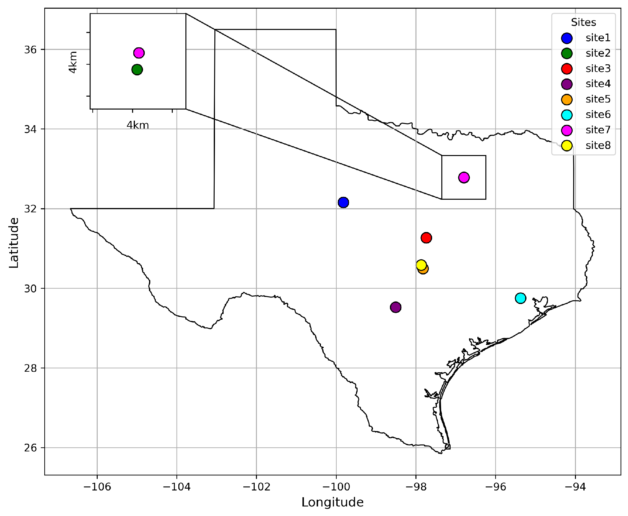
Texas has significant solar energy potential and deployed solar resources, with annual average global tilt solar radiation ranging from 4.76 kWh/m²/day to 6.58 kWh/m²/day across the state [40]. Its abundant solar resources, combined with the unique characteristics of the isolated ERCOT grid, make it an ideal region for this study. Eight sites across Texas were selected for analysis, with their locations and coordinates listed in

Table 1. Selected Sites and their Locations.

Name	Site	Latitude	Longitude
3-Door, Ovalo	1	32.154290	−99.81891
Camp David Dallas	2	32.776600	−96.79706
Hermitage Austin	3	30.26726	−97.74281
Kruckenland San Antonio	4	29.5213	−98.5101
Misty Morn Cedar Park	5	30.49450	−97.82257
Roof Station Houston	6	29.7554	−95.37575
Weather Toy Dallas	7	32.78709	−96.79605
Wiley, Leander	8	30.58262	−97.86712

, and their spatial distribution illustrated in Figure 2. In this study, Sites 2 and 7 share the same global 4 km² grid space, while each other site has a distinct global region.

The spatial distribution of the selected sites, shown in Figure 2, indicates that most of the sites are sparsely distributed across the region. However, certain locations—specifically Sites 3, 4, 5, and 8 form a relatively close cluster, while Sites 2 and 7 share the same global space as shown by the inset plot in Figure 2. Understanding this spatial arrangement is essential for accurately capturing the influence of neighboring sites on local conditions.

Table 2. Distances between sites (in km).

Site	1	2	3	4	5	6	7	8
1	0.00	291.81	219.76	318.32	264.60	500.59	292.17	254.71
2	291.81	0.00	190.04	396.97	271.69	362.07	1.17	264.13
3	219.76	190.04	0.00	207.62	86.26	282.26	191.11	77.05
4	318.32	396.97	207.62	0.00	126.86	304.03	398.07	133.25
5	264.60	271.69	86.26	126.86	0.00	249.26	272.81	10.69
6	500.59	362.07	282.26	304.03	249.26	0.00	363.12	256.55
7	292.17	1.17	191.11	398.07	272.81	363.12	0.00	265.25
8	254.71	264.13	77.05	133.25	10.69	256.55	265.25	0.00

presents the ground distances between the sites in km, further illustrating their relative proximity and separation.

The global dataset for each site was obtained from the NSRDB website [20], while the local dataset was sourced from Ambient Weather [41]. The global dataset consists of 5-min interval data on solar irradiance, temperature, pressure, wind speed, and dew point, spanning the period from 1 January 2022 to 31 December 2022. During the same period and with the same temporal resolution, ground-measured solar irradiance data were collected as the local irradiance dataset. The dataset for each site has 105,120 data points, enough to effectively train a machine-learning model.

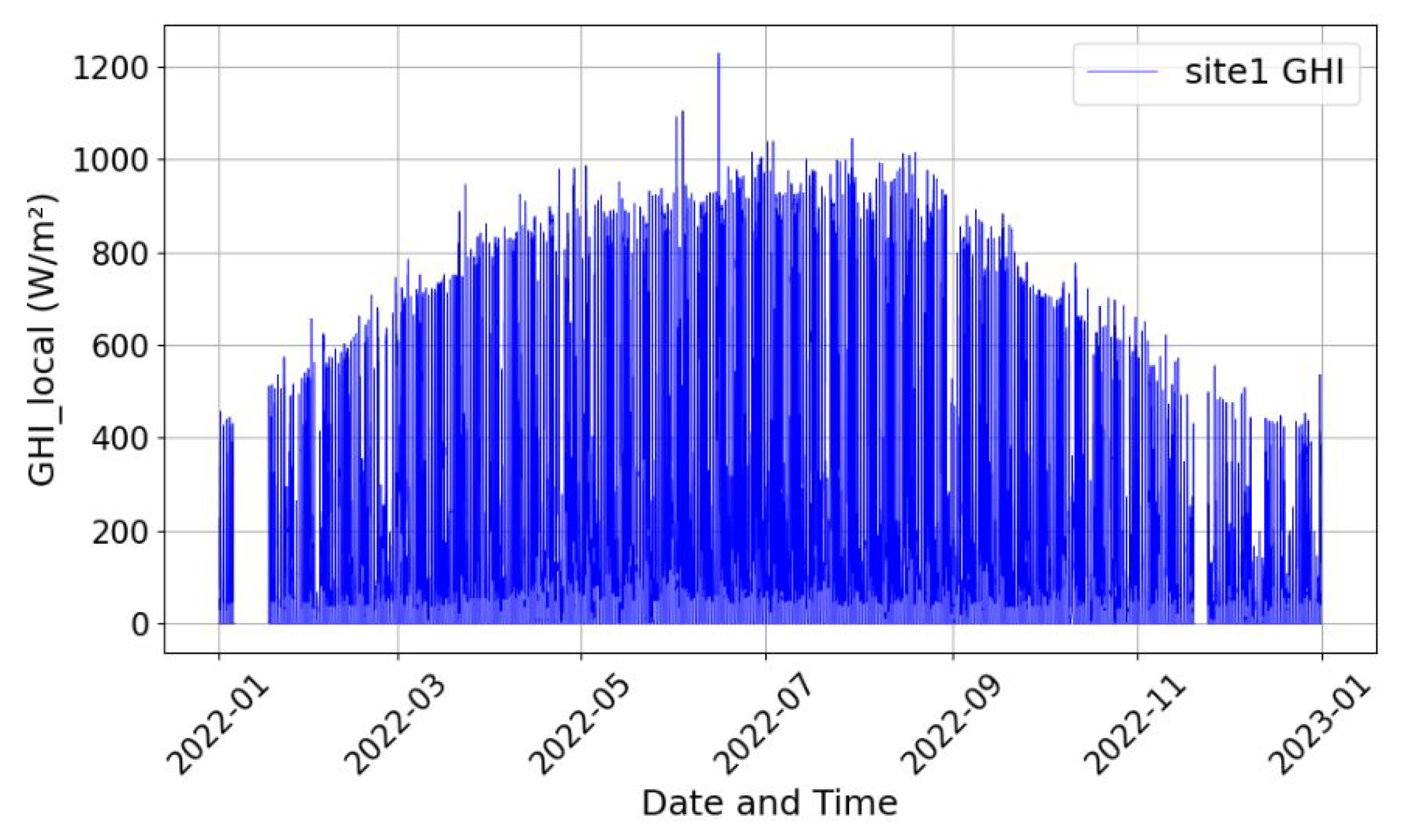
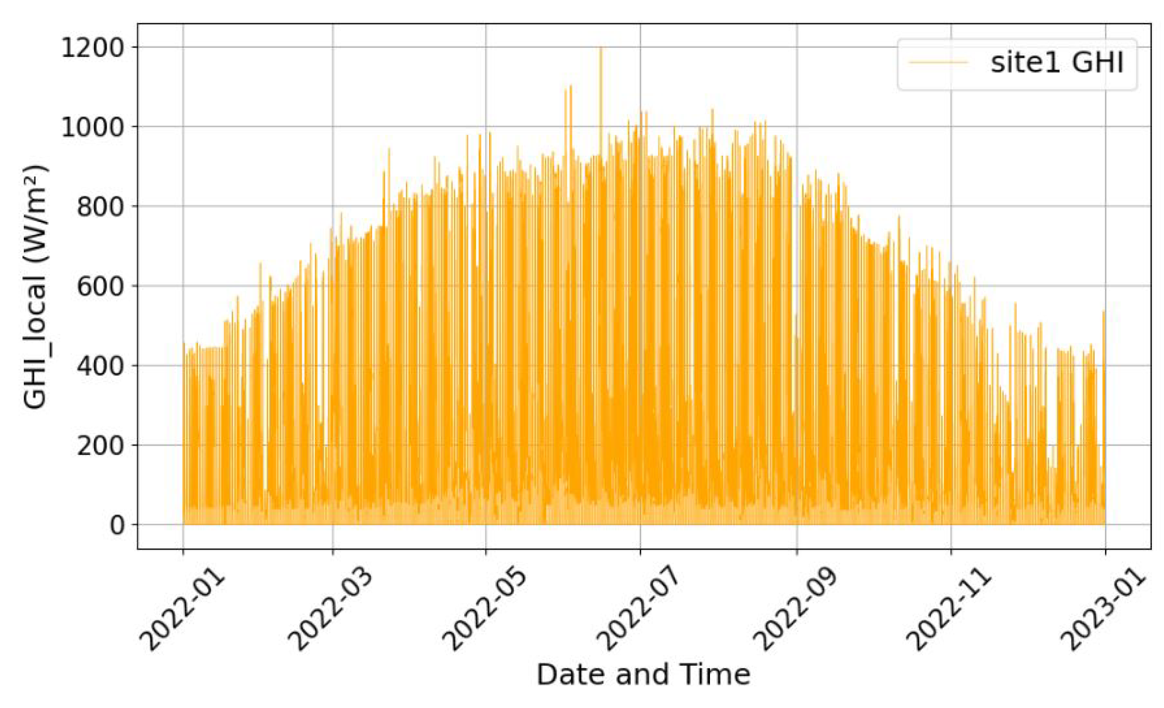
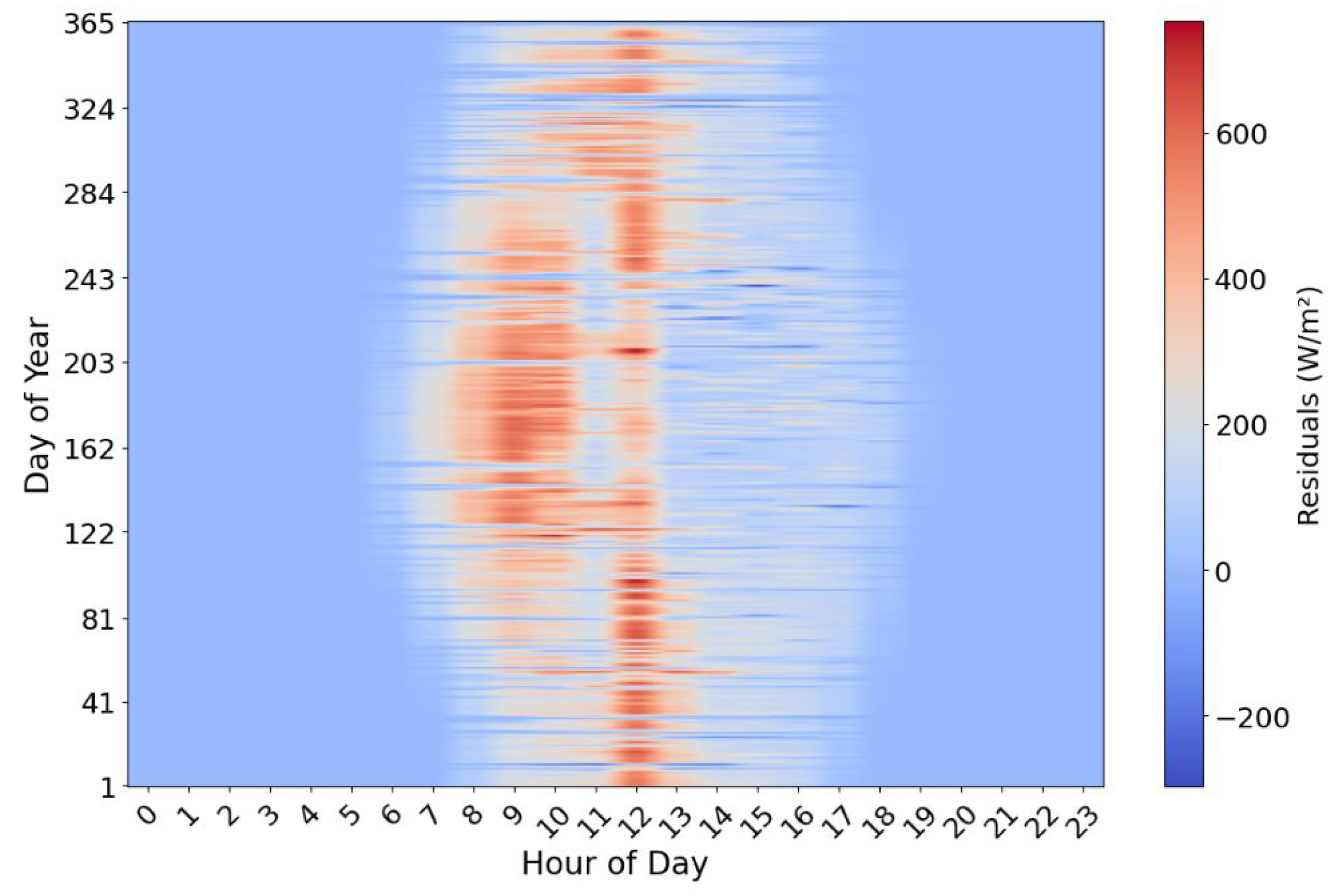
Figure 3 and Figure 4 present the annual profiles of global and local irradiance, respectively, for Site 1 in 2022. The plots show significant differences between the global and local irradiance. This is confirmed by the residual plot in Figure 5, which shows the numerical deviations of the global and local irradiance at each time point for Site 1. The global irradiance, being forecast values by NSRDB, does not accurately represent the ground measurements. In the same manner, the datasets of the other seven sites have similar distribution and deviation between the global and local irradiance. This observation reveals that the use of global solar irradiance for solar PV estimation could result in inaccurate solar PV forecasting, posing risks to power dispatch reliability and even network stability. This affirms the need to downscale the forecast global irradiance to more accurate site-specific values.

3.2. Feature Engineering

Solar irradiance is influenced by temporal and meteorological factors. Therefore, critical temporal features such as the hour of the day and day of the year were encoded using sine and cosine transformations to capture cyclical trends accurately. This cyclical encoding ensures continuity across periodic boundaries, such as midnight to midnight or December to January transitions. Capturing these cyclical temporal variations is crucial in reducing predictive errors, particularly during transitional periods with rapid changes in solar angles. Meteorological parameters such as temperature, atmospheric pressure, wind speed, and dew point from the global dataset were incorporated to reflect weather-dependent variability in irradiance. Integrating meteorological data provides essential contextual information that improves the model’s ability to generalize under diverse weather conditions and thus enhances its robustness. The Hour_sin and Hour_cos features were computed using equations:

$$\mathrm{Hour}\_\sin =sin\left({\displaystyle \frac{2\pi ·\mathrm{Hour}}{24}}\right),$$

(13)

$$\mathrm{Hour}\_\cos =cos\left({\displaystyle \frac{2\pi ·\mathrm{Hour}}{24}}\right).$$

(14)

Similarly, the DayOfYear_sin and DayOfYear_cos features were computed as:

$$\mathrm{DayOfYear}\_\sin =sin\left({\displaystyle \frac{2\pi ·\mathrm{DayOfYear}}{365}}\right),$$

(15)

$$\mathrm{DayOfYear}\_\cos =cos\left({\displaystyle \frac{2\pi ·\mathrm{DayOfYear}}{365}}\right).$$

(16)

The input data to the models are the encoded hour and day values, temperature, pressure, wind speed, dew point, and the global solar irradiance of the target and neighboring sites. These features were scaled using scikit-learn’s MinMax Scaler. The model was then trained to predict local solar irradiance as the output.

3.3. NNGP Implementation

The NNGP model was implemented to predict site-specific GHI values using a combination of spatial, temporal, and feature-based distances. For each site, its k-NNs were identified based on Euclidean distance in the spatial domain, with geographic coordinates serving as inputs. By focusing solely on these neighbors, the NNGP framework effectively localized the GP. This significantly reduced the dimensionality of the covariance matrices. Temporal dependencies were incorporated by considering the time difference between the current observation and historical data from neighboring sites. Temporal distances were calculated in minutes to ensure fine-grained temporal resolution suitable for solar irradiance modeling. Furthermore, feature-based distances were included to account for meteorological conditions such as temperature, pressure, wind speed, and dew point. These feature-based distances were computed in the feature-space to capture similarities and differences in environmental conditions across sites.

The squared exponential kernel in (5), used for the computation of the covariances incorporated spatial, temporal, and feature-based distances, with separate length-scale parameters (${\mathcal{l}}_s$, ${\mathcal{l}}_t$, ${\mathcal{l}}_g$, $\sigma$) for each distance type. Larger values of these parameters implied that distance neighbors and observations had a significant influence on the prediction outcome. These parameters, including the variance ($\sigma$), were tuned to balance their influence on the predictions. The final values of the hyperparameters used for the results in this paper are presented in

Table 3. Values of Hyperparameters for the NNGP model.

Hyperparameter	Value
number of neighbors (k)	3
$\sigma$	2.0
${\mathcal{l}}_s$	0.1
${\mathcal{l}}_t$	288 (1 day)
${\mathcal{l}}_g$	0.5
penalty term	0.2

.

To enhance the predictive capacity of the model, cyclical encoding of time was applied to represent the periodic nature of hours and days of the year. The covariance matrix among training points ($K_{\mathrm{train},\mathrm{train}}$) was regularized for numerical stability during inversion. Regularization was achieved by adding a small offset penalty term to the training covariance matrix to prevent singularities. Predictions were made using the GP regression formula provided in (6). This was achieved by combining the computed covariance matrices to scale the residuals between the neighbors’ local GHI and their predicted values from the linear regression model computed in (7). The resulting scaled residuals, known as the Gaussian correction term, were added to the linear regression estimated values of the target site to obtain the final downscaled GHI.

3.4. NNRF Implementation

Similar to the NNGP model, the NNRF model was developed to predict site-specific GHI values by leveraging spatial, temporal, and meteorological information. For each site, the model utilized its k-NNs, determined using Euclidean distances computed from the geographic coordinates of the sites. A k value of 3 was used in this model. This nearest-neighbor framework enabled the model to incorporate local spatial relationships, ensuring that predictions were informed by the most relevant neighboring data. Temporal dependencies were integrated by incorporating the encoded Hour and Day as part of the input features. This was carried out to ensure that training data reflected consistent diurnal and seasonal patterns. Additionally, meteorological features such as temperature, pressure, wind speed, and dew point were included to capture the environmental factors influencing solar irradiance variability.

The global GHI values of neighboring sites were also included as additional features to provide spatial context for each prediction. These neighbor features were aligned temporally to ensure consistency between the target site and its neighbors. The RF model, comprising an ensemble of decision trees, was trained using these features to predict the local GHI values. The model was initialized with 150 estimators to balance accuracy and computational efficiency. The ensemble approach enabled the RF model to handle complex non-linear relationships between input features and the target variable.

3.5. Scalability Test

Additionally, we investigated how well both models scale in terms of accuracy and computational speed with varying numbers of k-NNs. We achieved this by adding seven more sites to the existing ones to make fifteen, and retrained the models on a new dataset. To ensure adequate evaluation of the model’s scaling performance, the new training dataset was collected from 1 January to 30 December 2023, different from the former training dataset. Similar to earlier simulations, the dataset for 31 December 2023 was excluded to validate the accuracy of the scaled models. The k-NNs were varied from 2 to 14 for each of the sites. As a result of the increased data size, the scalability test was performed on one compute node of the South Dakota State University’s Innovator’s Cluster equipped with 2 Intel Xeon Gold 6342 CPUs with 48 cores. Each processor operated at a clock speed of 2.80 GHz and was supported by 256 GB of RAM.

3.6. Evaluation of Models

After the initial training of the two models on the dataset from 1 January 2022 to 30 December 2022, the models were validated by making day-ahead predictions of the downscaled local GHI for all eight sites for 31 December 2022. The evaluation of the model’s performance was achieved using Mean Absolute Error (MAE) and the Goodness of Fit (GoF). The MAE was computed as:

$$\begin{array}{c}\hfill \mathrm{MAE}={\displaystyle \frac{1}{N}}\sum _{i=1}^n|y_i-{\widehat{y}}_i|,\end{array}$$

(17)

where $y_i$ is the actual or true value of the i-th observation, ${\widehat{y}}_i$ is the predicted value corresponding to the i-th observation, and N denotes the sample size in the testing set. To measure how well the estimated models capture the patterns of the dataset, the GoF is computed using the normalized Root Mean Squared Error (NRMSE), such that:

$$\begin{array}{c}\hfill \mathrm{GoF}\left(Percent\right)=(1-\mathrm{NRMSE})\ast 100,\end{array}$$

(18)

where NRMSE is given by:

$$\begin{array}{c}\hfill \mathrm{NRMSE}={\displaystyle \frac{\sqrt{\frac{1}{n}{\sum }_{i=1}^n{(y_i-{\widehat{y}}_i)}^2}}{y_{\max }-y_{\min }}}.\end{array}$$

(19)

The use of the NRMSE to compute the GoF offers the advantage of normalizing the error to make it dimensionless, allowing easier comparison of the model’s performance across the dataset with different units. Additionally, while MAE, NRMSE, and GoF measure the effectiveness of the model, we assessed the model’s efficiency by measuring the computational time, as this is required for real-time power system operations.

3.7. Case Study on Puerto Rico

To evaluate the generalizability of the proposed data-driven models, it is essential to test their performance not only on unseen data but also across distinct climate zones. To this end, we conduct an additional validation using a new dataset from Puerto Rico, which represents a markedly different climatic environment compared to Texas. Puerto Rico was chosen due to its highly variable and erratic weather patterns, providing a test of the models’ robustness. Successful performance in this setting demonstrates the models’ ability to adapt to diverse environmental conditions. As with the Texas simulation, comparable datasets including global and local solar irradiance, as well as meteorological variables, were collected for this analysis. The data spans from 1 February 2023 to 31 December 2023, across five geographically distributed sites in Puerto Rico. Figure 6 presents the map of the selected locations.

Both the NNGP and the NNRF were trained on the dataset from Puerto Rico from 1 February 2023 to 31 December 2023. Similar to the earlier simulations, predictions were made for 31 December 2023. The hyperparameters of both models were maintained, but the number of decision trees for the RF was tuned from 100 trees to 150 trees.

4. Results and Discussion

4.1. Training Performance of NNRF and NNGP

Both the NNGP and NNRF perform very well during the training phase; however, the NNRF shows slightly superior accuracy over the NNGP. The performance of NNRF is consistently higher than NNGP across all eight sites, as could be seen from

Table 4. Comparison of NNRF and NNGP Training Performance.

Site	NNRF			NNGP
	MAE	NRMSE	GoF (%)	MAE	NRMSE	GoF (%)
1	13.6480	0.0278	97.22	19.8886	0.0479	95.21
2	8.1693	0.0178	98.22	12.7651	0.0303	96.97
3	13.5003	0.0256	97.44	20.5084	0.0446	95.54
4	11.9800	0.0271	97.29	19.0394	0.0475	95.25
5	12.0539	0.0245	97.55	20.7114	0.0441	95.59
6	13.6236	0.0250	97.50	20.4696	0.0432	95.68
7	5.9689	0.0183	98.17	9.2296	0.0316	96.84
8	12.4045	0.0235	97.65	19.6315	0.0410	95.90

. The NNRF records an average GoF of 97.63% across all sites, compared to 95.87% of the NNGP. This superior performance of the NNRF model can be attributed to RF’s ability to learn non-linear patterns in the dataset, in contrast to the NNGP’s inherent linearity. Furthermore, averaging the predictions of several decision trees makes the RF model robust to noise and outliers. This makes it comparatively more suitable for non-smooth data such as solar irradiance. Visual displays of the training performance of both models for Site 8 are shown in Figure 7a,b.

A careful observation of the two plots reveals how the NNRF model accurately captures the variability of the local irradiance better than the NNGP model. However, even though the RF model gives some partial interpretability in terms of the number of decision tree estimators and tree depth, the GP offers a better interpretability in terms of the correlation and influence of neighboring sites on predictions. The interpretability of NNRF can be further explored using explainable AI (xA), such as SHapley Additive exPlanations (SHAP) values [42]. The GP’s hyperparameters, such as the temporal, spatial, and feature length scales, and the variance, give visibility of how far in time-space or feature-space the model looks for correlations. Similarly, the covariance matrix’s structure reveals how points influence each other’s predictions.

This improved interpretability of the NNGP, however, comes with increased computational cost. The NNGP took 1004.19 s to train on the eight sites, compared to 407.63 s of the NNRF model. By avoiding the computation and inversion of covariance matrices, the NNRF model speeds up computational speed by 2.5 times more than the NNGP model. While these results are promising, validation is required to confirm how well they generalize and scale with an increasing number of neighboring sites, which is discussed later in the results.

4.2. Validation Performance of NNRF and NNGP

The final evaluation of the NNRF was made by predicting the downscaled local solar irradiance for the next day to be used in day-ahead power system operations. The dataset for 31 December 2022, used for this validation, was excluded from the training. The features of the global data and the global solar irradiance of the selected neighboring sites were used as input variables for the predictions. The day-ahead forecast was made for each site in a 5 min time step, and compared to the actual local solar irradiance of each site. The plots of the predicted downscaled solar irradiance for Sites 1, 2, 7, and 8 are presented in Figure 8. The orange line represents the NNGP’s predictions, and the red line depicts the predictions of the NNRF.

Table 5. Validation Results of NNRF and NNGP for Day-Ahead Forecast.

Site	NNRF			NNGP
	MAE	NRMSE	GoF (%)	MAE	NRMSE	GoF (%)
1	32.4447	0.1162	88.38	36.4148	0.1197	88.03
2	22.1226	0.0986	90.14	50.8843	0.2216	77.84
3	35.8097	0.1115	88.85	43.9536	0.1385	86.15
4	21.4388	0.0728	92.72	25.2055	0.0835	91.65
5	26.0342	0.1047	89.53	29.8221	0.1187	88.13
6	18.8950	0.0748	92.52	28.3873	0.1185	88.15
7	14.4113	0.1209	87.91	29.4329	0.2304	76.96
8	16.3520	0.0594	94.06	25.8150	0.0946	90.54

displays the model’s evaluation results for each site.

Once again, the NNRF performed better across all eight sites with an average GoF of $90.61\%$, compared to 86.31% of the NNGP model. This is confirmed by the plots in Figure 8, where the NNRF’s predictions closely follow the trajectory of the local GHI better than the NNGP model. The boxplots in Figure 9 show the residuals of the actual and predicted values. While each model’s residual has an approximate mean of 0, the variance of the NNGP is much larger than the NNRF (which appears in the other error metrics). Additionally, there are larger outliers predicted by NNGP, such as the −400 point in Site 1. All these observations confirm the superior performance of the NNRF model over the NNGP model.

Aside from these observations, the NNGP predictions show an interesting trend where it performed better for sites with less rapid variation in the local irradiance profile. Likewise, its performance is relatively lower for sites with rapid local irradiance variation, which deviates more from the shape of the global solar irradiance. For instance, as can be seen in Figure 8, Site 1 and Site 7, which recorded the lowest GoF, also display higher deviations from the profile of the global irradiance. This can be seen from

Table 6. Correlations Between Global and Local Solar Irradiance.

Site	1	2	3	4	5	6	7	8
Correlation	0.7635	0.9346	0.9543	0.9226	0.6487	0.9686	0.5797	0.9707

, where they show relatively lower correlation values of 0.7635 and 0.5797, respectively. Similarly, with the exception of Site 3, it is observed that the more the shape of the local and global irradiance is highly correlated, the higher the NNRF prediction’s accuracy. This implies that, generally, the alignment of the shape profiles of the global and local irradiance has a higher impact on the accuracy of prediction than the value of their variance. The MAE and the NRMSE also follow a similar pattern, where Site 7, whose profile’s shape deviates most from that of the global irradiance, recorded the highest prediction error. In sharp contrast, Site 8 records the minimum prediction error due to its high correlation value of 0.9707 between the global and local GHI.

This high correlation makes the global solar irradiance a good predictor of the local solar irradiance. However, when the local irradiance differs significantly from the global profile due to localized weather conditions such as cloud cover, terrain shading, or microclimate effects, the global irradiance features are unable to fully explain these local variations. The departure of Site 3 from this trend could be the result of a lower influence of the other features, such as wind, temperature, pressure, and dew point, on the predictions.

While the models’ performances are satisfactory, the variability in solar irradiance demands quantification of prediction uncertainty to improve grid planning. The NNRF model, though robust and more accurate, produces point estimates only. This makes it unable to give any insight into the prediction tolerance for effective planning or operation under uncertainties. The NNGP model, however, displays high strength in this regard. By using the values of the Gaussian corrections as variance, upper and lower bound prediction values could be generated by addition and subtraction with the mean values. These upper and lower bounds give some insight into the accompanying uncertainties of the predicted values. The results of the NNGP’s predictions for Site 3 and Site 4 are shown in Figure 10. This makes the NNGP model very suitable for probabilistic forecasts. Based on these results, the decision to choose NNRF or NNGP does not depend solely on factors such as accuracy, computational speed, and interpretability, but also, whether point forecasts or probabilistic forecasts are desirable.

4.3. Scalability of the NNGP and NNRF Models

The scalability results as presented in Figure 11 reveal how the NNRF consistently performs better than the NNGP model for different numbers of k-NNs. These accuracy values are the GoF of the day-ahead predictions of the NNGP and NNRF for 31 December 2023. It can be seen from Figure 11a that the NNRF requires as few as 3 k-NNs to achieve very good accuracy. Beyond 3 k-NNs, the NNRF model does not seem to record any significant improvement in prediction accuracy. Conversely, the NNGP accuracy scales linearly from 2 to 6 k-NNs, beyond which the accuracy shows very minimal improvement. If we select 3 k-NNs and 6 k-NNs as the local optimum values for the NNRF and NNGP, respectively, the corresponding accuracy is 90.13% for NNRF and 88.74% for NNGP. The equivalent computational time is 582.92 s for the NNRF and 1578.60 s for the NNGP. This clearly shows that besides requiring a smaller number of k-NNs to achieve a locally optimum accuracy, the NNRF also takes comparably less computational time (in this case, almost three times as fast as the NNGP model). Additionally, based on the results presented in Figure 11b, the NNRF scales linearly, whiles the NNGP displays a polynomial scaling with increasing number of k-NNs. This implies the NNRF responds to a step increase in the number of k-NNs with a scalar multiple of the computational time, while the NNGP responds with an exponential increase in the computational time. This further proves the effectiveness and efficiency of the NNRF model for large-scale solar irradiance downscaling tasks, making it more suitable for real-time grid integration of DERs.

4.4. Results of Puerto Rico Case Study

The NNRF model continued to outperform the NNGP model in both predictive accuracy and computational efficiency. Validation results yielded a Goodness of Fit (GoF) of 85.83% for NNRF compared to 84.79% for NNGP. Although the NNRF performance showed a slight decrease relative to its results in the Texas simulation, this reduction may be attributed to the increased volatility and rapid fluctuations in local solar irradiance observed in Puerto Rico. Nevertheless, the NNRF maintained a significant advantage in computational speed, completing the simulation in 276.1 s—nearly half the time required by the NNGP model, which took 530.8 s. These results further underscore the effectiveness of the proposed NNRF model in achieving comparable or superior accuracy while substantially reducing computational overhead. Figure 12 presents a visual comparison of the prediction performance of both models.

The results displayed in Figure 12 above are the point estimates of NNRF and NNGP. However, as stated earlier, the NNGP has the advantage of giving a probabilistic forecast that shows the prediction uncertainties to be expected. These are displayed in Figure 13 for Site 1 and Sites 5 in Puerto Rico.

Finally, we present the residual plot in Figure 14 to once again demonstrate how the NNRF gives lower prediction errors compared to the NNGP model.

5. Conclusions

This study evaluates the performance of the NNRF and NNGP models in downscaling solar irradiance to localized measurements. The NNRF model performs better than the NNGP model in terms of accuracy and computational time during both training and validation. The NNRF recorded an average validation accuracy of 90.61% which outperformed the 85.88% recorded by the NNGP model. The NNRF model also improved computational speed by 2.5 times over the NNGP model. A case study on five sites in Puerto Rico further confirmed the superior performance of the NNRF model over the NNGP model in terms of accuracy and computational speed. Although the NNGP lags behind in terms of accuracy and computational speed, it shows strength in terms of interpretability and prediction uncertainty quantification. Its hyperparameters, such as the variance ($\sigma$), temporal (${\mathcal{l}}_t$), spatial (${\mathcal{l}}_s$), and feature-based (${\mathcal{l}}_g$) scale parameters, give insight into how far in time and space past observations and neighboring sites influence the prediction outcome. This makes the NNGP more suitable for probabilistic estimates, which demands more transparency of the modeling process.

Furthermore, scalability tests that measured both models’ performance and computational speed with varying numbers of k-NNs from 2 to 14 showed a linear scaling for NNRF and a polynomial scaling for NNGP in terms of computational time. Similarly, the NNRF achieved a local optimal accuracy with 3 k-NNs, while the NNGP took 6 k-NNs to obtain a local optimal accuracy. Irrespective of the increased number of k-NNs, the NNGP still could not outperform the NNRF, which had a scaling accuracy of 90.13% compared to 88.74% of the NNGP. These findings prove the superiority of the NNRF for large-scale solar irradiance downscaling tasks. Further studies could investigate improving the NNRF’s accuracy by combining the nearest-neighbor model with either artificial neural networks, the extreme gradient boosting (XGboost) method, or other advanced machine-learning models.

These findings could be very useful in the implementation of the FERC order 2222, by enabling real-time, accurate estimation of solar PV capacity for day-ahead dispatch. Additionally, due to the improved accuracy and computational speed of the NNRF model, its application can be extended to the real-time electricity market with accurate PV estimates on a 5 min rolling basis. Finally, the use of downscaled solar irradiance forecasts reduces the level of solar PV generation uncertainties with its associated reserve requirements and instability issues in power dispatch planning.