Abstract
The existing linear frequency increment cable defect detection method using frequency domain reflectometry suffers from severe pseudo-peak phenomena due to non-targeted frequency domain sampling, which interferes with diagnosis. To address this issue, this paper proposes an optimized frequency domain sampling method based on the exponential frequency increment reflection coefficient spectrum. This method optimizes the distribution of frequency domain sampling points, reducing the sampling of high-frequency noise signals, thereby effectively suppressing pseudo-peaks. Research indicates that the low-frequency band of the cable reflection coefficient spectrum contains richer information about the cable’s condition and has less noise compared to the high-frequency band. Therefore, an exponential frequency increment is used instead of the current linear frequency increment, resulting in a denser sampling in the low-frequency band and sparser sampling in the high-frequency band, better matching the information distribution characteristics of the cable reflection coefficient spectrum. To avoid spectral leakage caused by non-uniform sampling under exponential frequency increments, this method locally linearizes exponential sampling and uses interpolation to complete the overall frequency sampling rate, ensuring it meets the basic assumption of Fourier transform—uniform and equally spaced sampling signals. Finally, this method was validated on a 500 m laboratory test cable and a 2000 m operational cable. Experimental results show that this method can make the amplitude of regions other than impedance mismatch points in the positioning curve flatter and effectively suppress abnormal peak interference, significantly improving the accuracy of defect diagnosis.
1. Introduction
With the development of urbanization and the large-scale aging of cables, there is an urgent need for rapid cable defect location. In recent years, the frequency domain reflection method (FDR) has been widely used in cable defect detection and has been proven to be a reliable and effective defect location method through numerous field cases [1,2,3]. However, FDR still has some issues: the maximum inherent frequency of different types and lengths of cables varies, making it difficult to ensure linear sampling for each cable in actual testing [4]; high-frequency signals attenuate quickly, leaving only noise during propagation [5], so more high-frequency signals are not necessarily better for cable location; high-frequency signals generate strong multiple reflections at the front and near ends, creating many abnormal peaks that affect judgment. Therefore, reducing high-frequency signal attenuation and suppressing the impact of abnormal peaks are crucial for accurate cable defect location and diagnosis.
Ohki et al. initially measured the broadband input impedance of cables through frequency domain scanning and used inverse fast Fourier transform to detect cable aging areas [6,7]. However, this method requires sweep frequency equipment with a large test frequency range and many test frequency points, increasing testing costs and limiting its application scope. Hernández-Mejía et al. created defects on cables using local heating and used frequency domain reflection and inverse fast Fourier transform to precisely locate the defects, proving that increasing the incident signal frequency can effectively improve the spatial resolution of the location spectrum [8]. Zhou Kai et al. proposed a method for selecting the optimal upper frequency limit [9], effectively reducing cable defect location errors, but in actual testing, the optimal upper frequency limit of the test cable cannot be obtained and can only be estimated based on experience. Li Chengrong et al. proposed a cable local defect location method based on frequency-modulated continuous waves, enhancing the anti-interference capability of the test signal, but the cable detection distance is limited, making it unsuitable for actual cable detection and unable to solve the problem of abnormal peak interference.
To address these challenges, this study introduces a novel cable defect localization approach utilizing an exponentially increasing frequency-based reflection coefficient spectrum. Low-frequency signals attenuate more slowly compared to high-frequency signals, resulting in the reflection coefficient spectrum containing richer cable status information (including amplitude and phase characteristics) in the low-frequency band than in the high-frequency range. Additionally, within the low-frequency domain, the amplitude variations in the reflection coefficient spectrum better align with the signal attenuation trend. However, in high-frequency regions, the amplitude–frequency curve becomes susceptible to distortion, which alters the cable state information and introduces measurement errors. By controlling the sampling method of the injected signal, the effects of spectral leakage and abnormal peaks are suppressed. This method differs from traditional linear frequency increments by making the frequency increase exponentially, resulting in dense low-frequency sampling and sparse high-frequency sampling, better matching the information distribution characteristics of the cable reflection coefficient spectrum. Interpolation is then used to complete the overall frequency sampling rate, ensuring it meets the basic assumption of Fourier transform—uniform and equally spaced sampling signals. Finally, the method is tested on a 500 m laboratory test cable and a 2000 m operating cable. The results show that the method effectively suppresses the generation of abnormal peaks, which proves the effectiveness and practicability of the method.
2. Traditional Linear Frequency Increment Defect Location Method
2.1. Cable Distributed Parameter Model
According to transmission line theory [10,11,12], a cable can be considered as composed of countless tiny segments, each with specific distributed parameters, including resistance R0, conductance G0, capacitance C0, and inductance L0 per unit length Δx, as shown in Figure 1. These tiny segment equivalent circuits are cascaded to simulate the electrical characteristics of the cable under high-frequency conditions. The approximate formulas for the resistance R0 (Ω/m), inductance L0 (H/m), conductance G0 (S/m), and capacitance C0 (F/m) per unit length of the cable have been fully derived in the literature [13] and will not be repeated here.
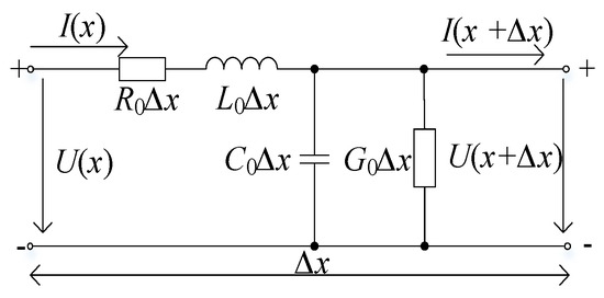
Figure 1.
Equivalent model of cable distribution parameters.
2.2. Principle of Linear Frequency Increment Defect Location
Based on transmission line theory, the reflection coefficient Γl at the input terminal of a cable with a length of l can be expressed as [14]
where ZL represents the load impedance, γ denotes the propagation constant of the cable, and Z0 stands for the characteristic impedance of the cable, which can be defined as
where α is the attenuation factor, representing the signal amplitude attenuation characteristics per unit cable length; β is the phase constant, representing the signal phase lag characteristics per unit cable length [15]; and v is the speed of electromagnetic waves in the cable, which is constant at high frequencies.
When the cable end is open (ZL = ∞), Γl can be expressed as
Expanding Equation (3) using Euler’s formula and taking the real part gives the reflection coefficient spectrum at the front end of the cable:
where Real(Γl) is the real part of the reflection coefficient Γl, and f is the test frequency. From Equation (4), it can be seen that Real(Γl) exhibits an exponentially decaying oscillation. When the test frequency f is the independent variable, the real part of the reflection coefficient of a healthy cable will have a frequency equivalent component of 2 l/v. When there is an impedance discontinuity at a distance l1 from the front end of the cable, such as a defect or fault, the real part of the reflection coefficient will have a frequency equivalent component of fl1 = 2 l1/v. This corresponds to the round-trip propagation time of the input signal traveling from the cable’s front end to the impedance discontinuity located at a distance l1 and back. The defect location in the cable can be determined using the following equation:
Consequently, the impedance discontinuity along the cable can be accurately identified by conducting Fourier analysis on the real component of the reflection coefficient.
2.3. Problems with Linear Frequency Increment
The low-frequency band of the cable reflection coefficient spectrum contains richer cable state information and less noise, while the traditional frequency domain reflection method does not prioritize frequency points, giving equal weight to the entire frequency band. The maximum inherent frequency of different types and lengths of cables varies, making it difficult to ensure linear sampling for each cable in actual testing. Since high-frequency signals attenuate quickly during propagation in the cable, only low-frequency signals and noise remain during long-distance cable propagation. If a continuous linear frequency increment sampling method is used, considering signal attenuation, a higher upper frequency limit cannot be set, but this will result in poor resolution between location peaks due to the lack of high-frequency signals, and the obtained location peaks will be too wide, obscuring adjacent defect segments. To improve the resolution between location peaks, a higher upper frequency limit is needed, but this will increase the number of high-frequency components, accelerating the overall signal attenuation and leaving only noise, affecting the diagnosis of long-distance cables. At the same time, high-frequency signals generate strong multiple reflections at the front and near ends, creating abnormal peaks that affect judgment.
The amplitude–frequency characteristics of the reflection coefficient spectrum are shown in Figure 2. It can be seen that the low-frequency band contains richer information about the amplitude, phase, and signal attenuation of each frequency point in the cable reflection coefficient spectrum, while the high-frequency band is distorted due to signal attenuation and noise interference, making it unfavorable for reflecting the actual condition of the cable [16,17]. Therefore, in actual measurements, more low-frequency signals and fewer high-frequency signals should be included to avoid the impact of signal attenuation and noise interference on the test results, allowing the reflection coefficient spectrum to reflect more effective cable state information.
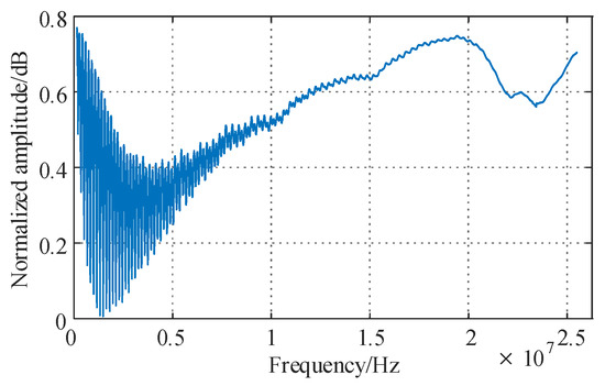
Figure 2.
Amplitude–frequency characteristics of reflection coefficient spectrum (measured).
3. Exponential Frequency Increment Defect Location Method
Therefore, an exponential frequency increment frequency domain sampling optimization method is proposed, increasing the frequency selection interval according to an exponential growth trend, resulting in a higher density of low-frequency sampling points and a sparser distribution of high-frequency sampling points within the same total number of measurement points, better matching the information distribution characteristics of the cable reflection coefficient spectrum. To facilitate fast Fourier transform data processing, multiple equally spaced linear samplings are used to replace exponential sampling, making the frequency trend increase exponentially while maintaining local uniform sampling. Interpolation is then used to complete the overall frequency sampling rate, improving the sampling rate and frequency resolution, further reducing the interference of abnormal peaks caused by spectral leakage.
3.1. Exponential Frequency Increment
The frequency of the exponential frequency increment sweep signal increases exponentially with time, and its time-domain expression is as follows:
where A denotes the signal amplitude, f0 represents the initial frequency, a is the base of the exponent function, k is a constant governing the rate of frequency variation, t signifies time, and β corresponds to the initial phase. To explore more accurately the influence of various parameters of the index-increased swept-frequency signal on the reflection coefficient spectrum, the following discussion is carried out:
- Selection of Signal Amplitude (A): This parameter solely affects the upper and lower clipping levels of the input signal. As indicated by Equations (2), the cable’s propagation constant and characteristic impedance are independent of signal amplitude. Moreover, higher amplitude values for high-frequency test signals require greater power delivery capabilities, which become increasingly challenging to implement. To standardize parameter configurations, the input voltage of the FDR test equipment (Sichuan University, Chengdu, China) is set to 5 V; hence, the signal amplitude is designated as A = 5 V in subsequent analyses.
- Selection of Initial Frequency (f0): The lower frequency limit of the network analyzer employed in laboratory settings is 150 kHz. Consequently, the initial frequency is configured as f0 = 150 kHz for both simulations and experimental validations.
- Determination of Frequency Ramp Rate (k): Equation (6) demonstrates that parameter k essentially equivalates to modifying the effective starting frequency. For computational convenience, the frequency ramp rate is standardized at k = 1 throughout subsequent simulations and experimental procedures.
- Specification of Initial Phase (β): As derived from Equation (6), the initial phase parameter exerts no influence on test signal characteristics when implementing continuous sinusoidal frequency-sweep excitation. To facilitate analytical processing and computational efficiency, the initial phase is designated as β = 90°.
In conclusion, Equation (6) can be simplified as follows:
The time-domain waveform and time-frequency characteristics of the exponential frequency increment sweep signal are shown in Figure 3 and Figure 4. It can be seen that in the time domain, the period of the exponential frequency increment signal becomes denser over time. This means that in the frequency domain, the interval between each frequency component increases exponentially over time. Such a distribution can make the spectrum energy more concentrated in the low-frequency part after Fourier transform, reducing spectral leakage in the low-frequency part. The high-frequency part, due to its fast energy attenuation and low amplitude after FFT, will not exceed the amplitude of the main lobe even if spectral leakage is exacerbated by sparse sampling, thus suppressing the generation of abnormal peaks to some extent. At the same time, the low-frequency signal in the cable reflection coefficient spectrum contains richer cable state information. Therefore, under the same impedance sampling bandwidth and frequency domain sampling points, this method can obtain more cable state information compared to traditional linear frequency increments, thereby increasing the accuracy of defect location.
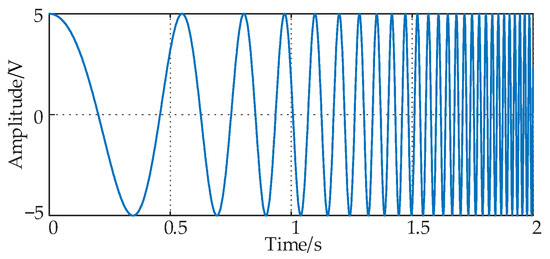
Figure 3.
Time-domain waveform of exponential frequency increasing signal.
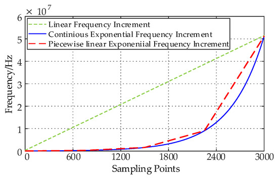
Figure 4.
Time-frequency characteristics of exponential frequency-increase signal.
3.2. Local Linearization of Exponential Frequency Increment
As shown in Figure 4, the exponential frequency increment signal contains more low-frequency components and some high-frequency components. However, when using exponential frequency increments for frequency selection, since the windowed Fourier transform assumes that the input signal is uniformly sampled with equal intervals between frequency points, directly using the windowed Fourier transform will affect the transformed results [18]. Therefore, based on the exponential frequency increment, a local piecewise linear frequency increment sampling method is used, and its time-frequency characteristics are shown in Figure 4. This method can achieve equally spaced sampling during windowed Fourier transform while still meeting the frequency distribution requirements of more low-frequency components and fewer high-frequency components according to the exponential growth trend.
In terms of parameter settings, compared to the traditional linear continuous frequency increment method, the base of the exponential function and the number of linear segments need to be determined, and the selection of these two parameters will directly affect the quality of the exponential frequency increment.
For the selection of the base of the exponential function, it is necessary to balance the frequency growth rate and signal power attenuation. Choosing a base that is too high will cause the frequency to grow too fast, possibly missing too much mid-to-high frequency information, thus losing details of the near end of the cable. The signal power attenuation can be calculated using the following formula:
where αc is the attenuation coefficient of the cable.
To ensure the effectiveness of data processing, it is necessary to ensure that each piecewise linear exponential frequency increment signal contains enough frequency components. Therefore, the range of the base is limited to between 1 and 10, and the base is selected in steps of 0.1. Through step experiments, the impact of different bases from 1.1 to 10 on signal power attenuation and frequency growth rate is evaluated.
As illustrated in Figure 5, the energy attenuation exhibits a nonlinear oscillatory relationship with varying exponential bases. When the base is set to 2, the signal energy attenuation reaches its minimum value of 0.488. To further validate the suitability of the frequency growth rate under this base, a 600 m cable is analyzed. Based on the measured amplitude–frequency characteristics of the reflection coefficient spectrum, the curve above 20 MHz demonstrates irregular distortions, rendering the extraction of effective cable state information impractical. Consequently, the cut-off frequency is standardized at 20 MHz, with an initial frequency of 150 kHz and a sampling point count of 3000. The frequency growth curve with a base of 2 is plotted in Figure 6.
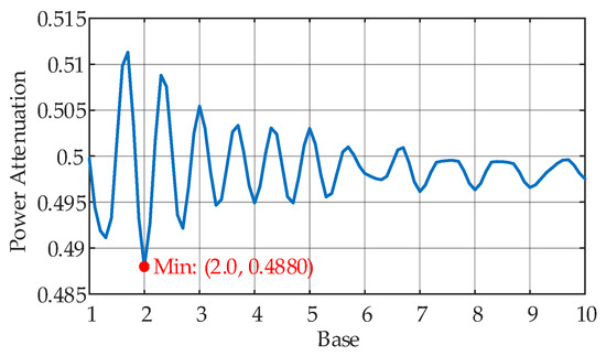
Figure 5.
Optimal Selection Curve for exponential base.
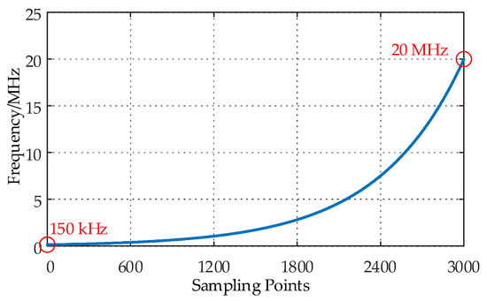
Figure 6.
Frequency growth curve with exponential base number of 2.
Furthermore, Figure 2 reveals that the low-frequency range (150 kHz to 5 MHz) encompasses richer cable state information, including reflection coefficient spectral amplitudes, phase characteristics, and attenuation profiles. Specifically, the 150–10 MHz frequency band contains the majority of valid cable state information. As shown in Figure 6, when using a base of 2, the low-frequency portion (≤10 MHz) occupies 71.6% of the total sampling points, significantly surpassing the 25% achieved by linear frequency increments. Additionally, the effective cable information bandwidth accounts for 85.8% of the total sampling points, far exceeding the 50% observed with linear frequency progression. These results confirm that the frequency growth rate with a base of 2 is highly appropriate.
In conclusion, based on comprehensive analysis of energy attenuation minimization, frequency distribution optimization, and sampling efficiency, a base value of 2 is determined to be the optimal choice for this application.
The number of linear segments is determined as follows:
- 1.
- Select the initial number of segments: first, determine an initial number of segments based on the characteristics of the exponential frequency increment signal or testing experience.
- 2.
- Piecewise linear fitting: calculate the frequency of each segment point based on the start, stop frequency, and number of segments, and then use linear interpolation to perform piecewise linear fitting on the signal.
- 3.
- Calculate the fitting error: Introduce an error function to measure the difference between the piecewise linear function and the original exponential frequency increment signal. Use the root mean square error (MSE) to calculate the fitting error.
- 4.
- Optimize FFT calculation overhead: optimize through iterative experiments, evaluate the FFT calculation overhead under different numbers of segments, and the FFT calculation complexity (O(N/log N)) is usually related to the number of data points, so the FFT calculation time can be compared for evaluation.
- 5.
- Determine the optimal number of segments: balance the selection of calculation overhead and approximation accuracy to find a compromise that provides good fitting and optimizes FFT calculation overhead.
Among them, S is the number of segments, E(S) is the fitting error function, which measures the difference between the piecewise linear function and the original exponential frequency increment curve. C(S) is the FFT computation cost function, which measures the computational resource consumption for performing the FFT transformation. w1 and w2 are weighting coefficients used to balance the importance of fitting error and computation cost. The parameter setting flow chart is shown in Figure 7.
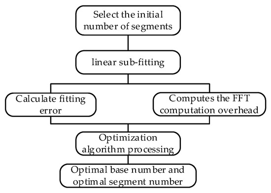
Figure 7.
Parameter setting flow chart.
To determine the optimal number of segments, a 600 m cable was analyzed using parameters from the previous section: frequency band 150–20 MHz, 3000 sampling points, exponential base 2, and the frequency growth curve in Figure 6 as the reference. Piecewise linear fitting was performed with segment counts ranging from 3 to 15, yielding the segment-dependent MSE and computation time curves in Figure 8.
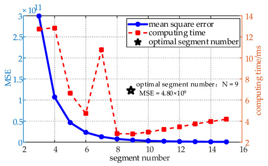
Figure 8.
The influence of the number of segments on the fitting error and calculation time.
As shown in Figure 8, the MSE decreases nonlinearly with increasing segments, exhibiting significant initial reduction before plateauing beyond 10 segments. Computation time shows no linear correlation but follows a trend: sharp decline initially, followed by a gradual rise after nine segments. At nine segments, MSE = 4.8 × 10⁹. Given the large frequency unit scale, the absolute error is approximated as 6.9 × 10⁴ Hz, corresponding to a relative error of 0.34% (relative to 20 MHz), which is acceptable for practical localization. Increasing to 10 segments reduces the MSE to 3.2 × 10⁹ (0.29% error), but computation time rises by 18% (2.7 ms to 3.2 ms). This delay would amplify in real-world testing.
Thus, nine segments achieve the shortest computation time with sufficient accuracy, making it the optimal choice for 600 m cable measurements.
After using this method for frequency selection, during data processing, each linear segment of data is interpolated at equal intervals to restore the reflection coefficient spectrum to the set frequency band range with equally spaced sampling results, as shown in Figure 9. It can be seen that although the reflection coefficient spectrum of the linear frequency increment method shows a relatively standard attenuation curve, due to the limitation of the number of sampling points, the amplitude–frequency curve of the reflection coefficient spectrum still has amplitude distortion; before interpolation, the exponential frequency increment method has fewer sampling points in each linear frequency segment, missing many frequencies, resulting in obvious amplitude mutations in the amplitude–frequency characteristic curve of the reflection coefficient spectrum; after cubic spline interpolation, the exponential frequency increment method eliminates the problem of data missing due to fewer sampling points of high-frequency signals, making the amplitude–frequency curve of the reflection coefficient spectrum smoother, and the frequency sampling rate is completed to equally spaced sampling, improving the sampling rate and frequency resolution, which means that adjacent frequency components can be more clearly distinguished in the spectrum. In this way, even if spectral leakage occurs, its impact on the analysis results becomes less significant due to the higher resolution, thereby reducing the impact of spectral leakage on location analysis.
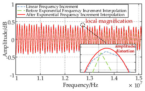
Figure 9.
Reflection coefficient spectrum amplitude–frequency characteristic curves of different methods.
4. Cable Defect Simulation Verification
4.1. Simulation Parameter Settings
Common cable body defects change the local unit capacitance C of the cable, forming impedance discontinuity defects. The normal cable unit capacitance is C0, and the unit capacitance at the defect changes. To illustrate that the local linear exponential frequency increment method can suppress the generation of abnormal peaks while ensuring the same location error, simulation experiments are conducted on cables with total lengths of 300 m and 600 m based on the cable distributed parameter model. The defect parameters with the same multiple of capacitance increase are set to facilitate the judgment of the impact of different methods on signal attenuation. The simulation parameters for the cable are summarized in Table 1, with the values for R0, L0, G0, and C0 derived from established literature [19] sources.

Table 1.
Cable simulation parameters.
According to the linear segment selection method described in Section 2.3, for Cable 1, a suitable frequency range of 50–51.2 MHz is selected based on its length, and then the linear segment fitting error and FFT calculation overhead are calculated using the iterative algorithm to obtain the optimal number of segments as eight. Similarly, for Cable 2, the optimal number of segments is nine.
4.2. Simulation Result Analysis
For the single defect set on Cable 1, two methods are compared, and the same upper frequency limit is set. The location curves are shown in Figure 10, where the linear frequency increment method has 10,000 measurement points, and the exponential frequency increment method has 1800 measurement points, using interpolation to increase to 200,000 points. Compared to the linear frequency increment method, the exponential frequency increment method has fewer measurement points while ensuring the same location error. To eliminate the impact of using only interpolation on the location effect, the linear frequency increment method is also interpolated to the same number of points. It can be seen after interpolation that there is not much difference from the original linear frequency increment curve, indicating the necessity of selecting frequencies according to the exponential trend. At the same time, it can be seen from the figure that the exponential frequency increment method effectively suppresses the side lobe effect caused by large end reflections, making the amplitude of regions other than the defect smoother and the location map simpler. This is because the dense low-frequency sampling and sparse high-frequency sampling reduce spectral leakage in the low-frequency part. At the same time, the low-frequency part has concentrated energy and slow attenuation, resulting in a larger amplitude after FFT; the high-frequency part has dispersed energy and fast attenuation, resulting in a lower amplitude after FFT, so even if the high-frequency part has increased spectral leakage due to sparse sampling, it will not exceed the amplitude of the main lobe, thus achieving a certain suppression effect and obtaining a smoother location curve.
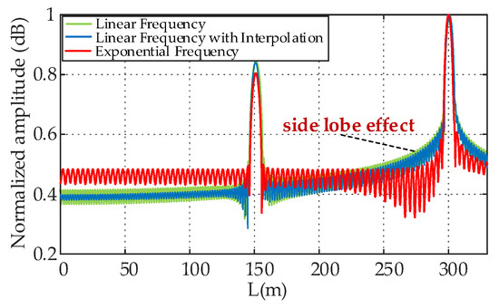
Figure 10.
Linear frequency-increasing and exponential frequency-increase positioning curves of Cable 1.
For the multi-defect model, the defect setting method is as described in Section 3.1, and the parameter setting method is as described in Section 3.2. The frequency range of 50–25.6 MHz is selected, and the defect location curve of Cable 2 is shown in Figure 10. The exponential frequency increment method has 1912 measurement points, using interpolation to increase to 100,000 points, and the linear frequency increment method has 10,000 measurement points, with an additional linear frequency increment curve interpolated to the same number of points. From Figure 11, it can be seen that when there are multiple defects, using the linear frequency increment method in the Fourier transform process will cause spectral leakage in both the high-frequency and low-frequency parts due to the same sampling rate across the entire frequency band but limited by the number of sampling points, generating abnormal peaks and affecting the accuracy of location. At the same time, the side lobe effect causes the amplitude of regions other than impedance mismatch points to be abnormally raised by the influence of these points, increasing the misjudgment rate of defect location. When using the exponential frequency increment method, there are more low-frequency components and fewer high-frequency components with a large span. Such a distribution can make the spectrum energy more concentrated in the low-frequency part after Fourier transform, reducing spectral leakage in the low-frequency part. After interpolation, the frequency resolution is completed to equally spaced sampling, further reducing spectral leakage, significantly reducing the impact of side lobes and abnormal peaks on the location effect.
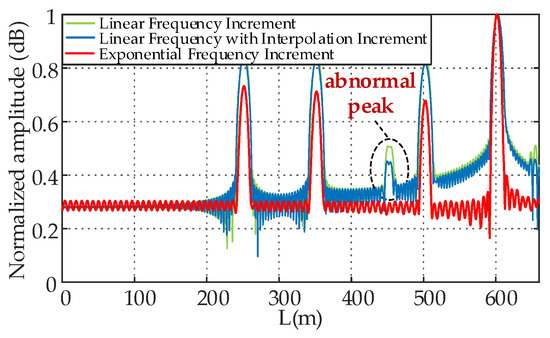
Figure 11.
Positioning curves of Cable 2 using both linear frequency-increasing and exponential frequency increment methods.
5. Power Cable Experimental Verification
5.1. Laboratory 500 m 10 kV XLPE Cable Experimental Verification
As shown in Figure 12, a 500 m long YJLV22 8.7/15-1 × 95 10 kV XLPE power cable is tested in the laboratory, with a middle joint made at 250 m. The test frequency range is 150–25.5 MHz, the exponential frequency increment method has 1580 sampling points, and the traditional linear frequency increment method has 10,000 sampling points.
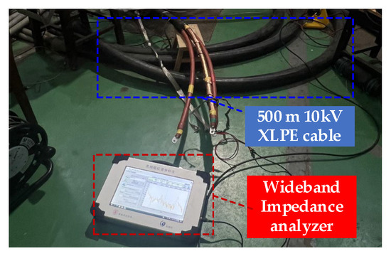
Figure 12.
500 m Cable Test Platform.
The FDR test results are shown in Figure 13. As illustrated in the figure, the exponential frequency increment method significantly reduces the amplitude in regions outside the joint and the cable end compared to the linear frequency increment approach, effectively mitigating the influence of side lobes on the localization results. In terms of localization accuracy, the traditional linear frequency increment method estimates the total cable length as 502.8 m, with the joint positioned at 251.3 m, resulting in a localization error of 0.54%. In contrast, the exponential frequency increment method achieves a total length estimate of 501.1 m, a joint position of 250.4 m, and a reduced localization error of 0.19%. Furthermore, the testing time is decreased from 10.3 s to 3.1 s, representing a 69.9% reduction, thereby significantly lowering time costs. When applied to the measurement of cable groups, such as in the case of 100 cables, the time savings directly determine whether the measurements can be completed within the allocated timeframe, enhancing measurement efficiency and improving the fault tolerance of on-site operations.
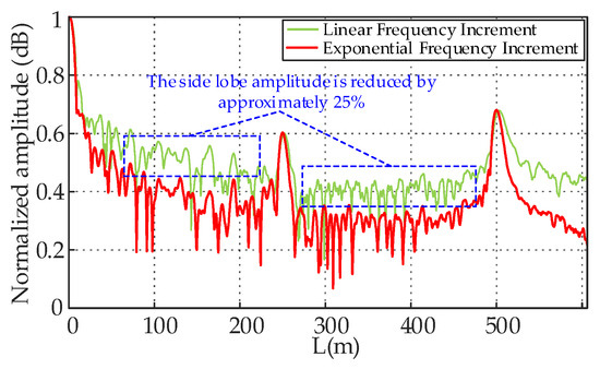
Figure 13.
Positioning map of 500 m cable.
5.2. In-Service 2000 m 10 kV XLPE Cable Experimental Verification
To verify the engineering practicality of the proposed method, an in-service cable is tested. The cable is 2000 m long, model YJLV22 8.7/15-1 × 95 10 kV XLPE power cable, and the test frequency range is 150–12 MHz. Operational site testbed is shown in Figure 14. The FDR test result is shown in Figure 15.
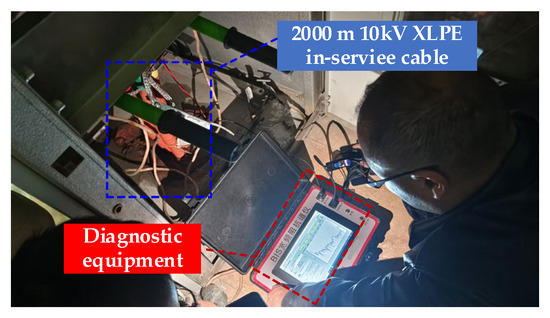
Figure 14.
Operational site testbed.
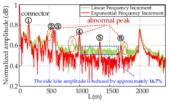
Figure 15.
Positioning map of the 2000 m cable in service.
From the figure, it can be seen this method lowers the amplitude of regions other than the joint and the end, to some extent suppressing the impact of side lobes on the location result. Combined with on-site record information and location curve joint diagnosis, it is determined that the peaks at 500 m and 900 m on the linear frequency increment are abnormal peaks caused by multiple reflections of the joint at 100 m, while the other peaks correspond to the joint positions in the records, thus verifying the suppression effect of this method on abnormal peaks. At the same time, the overall test time is reduced from 9.8 s to 3.4 s, a reduction of 66.7%, reducing the overall test time cost. In summary, it can be seen that the exponential frequency increment method is superior to the traditional linear frequency increment method in terms of reducing location error, the abnormal peak suppression effect, and overall test time.
6. Conclusions
This paper proposes a cable sampling frequency optimization method based on the exponential frequency increment reflection coefficient spectrum to solve the problem of traditional linear frequency scanning methods in cable defect detection being unable to accurately locate due to excessive side lobe amplitude and abnormal peaks caused by spectral leakage. By using non-linear exponential growth frequency sampling, dense low-frequency sampling and sparse high-frequency sampling are achieved, effectively reducing spectral leakage in the low-frequency band. Experimental results show that this method can effectively suppress the amplitude fluctuation of regions other than impedance mismatch points in the location curve on a 500 m laboratory cable and a 2000 m in-service cable, significantly reducing the interference of abnormal peaks and reducing location error.
Author Contributions
Conceptualization, K.J., K.Z. and Y.X.; methodology, K.J., K.Z. and Y.X.; resources, K.Z. and Y.X.; data curation, K.J.; writing—original draft preparation, K.J.; writing—review and editing, K.Z. and Y.X.; supervision, K.Z. and Y.X.; project administration, K.Z. and X.R.; funding acquisition, K.Z. and X.R. All authors have read and agreed to the published version of the manuscript.
Funding
This research was funded by the Science and Technology Project of State Grid Corporation of China (Research and Application of High Voltage Cable Typical Defect Detection and Location Technology Based on Time-Frequency Information of Increased Frequency Pulse, Grant No. 5500-202422152A-1-1-ZN).
Data Availability Statement
The data presented in this study are available on request from the corresponding author due to privacy.
Conflicts of Interest
Author Xiang Ren is employed by the company State Grid Hubei Electric Power Co., Ltd. The remaining authors declare that the research was conducted in the absence of any commercial or financial relationships that could be construed as a potential conflict of interest. The funding sponsors had no role in the design of the study; in the collection, analyses, or interpretation of data; in the writing of the manuscript, and in the decision to publish the results.
Abbreviations
The following abbreviations are used in this manuscript:
| FDR | Frequency Domain Reflection |
| FFT | Fast Fourier Transform |
| MSE | Mean Square Error |
| XLPE | Cross-Linked Polyethylene |
References
- Liu, F.L.; Xia, R.; Li, W.J. Research on Detection Method of Buffer Layer Ablation Defect in High Voltage XLPE Cable. High Volt. Appar. 2022, 58, 259–266+274. [Google Scholar]
- Zhao, S.J.; Zhan, B.B.; Gong, L.T. Research on Cable Local Defect Detection Method Based on Phase-Sensitive Characteristics of Frequency Modulated Continuous Wave. Trans. China Electrotech. Soc. 2023, 38, 3009–3021. [Google Scholar]
- Hu, Y.X.; Chen, L.; Liu, Y.; Xu, Y. Principle and Verification of an Improved Algorithm for Cable Fault Location Based on Complex Reflection Coefficient Spectrum. IEEE Trans. Dielectr. Electr. Insul. 2023, 30, 308–316. [Google Scholar] [CrossRef]
- Zhou, Z.Q. Local Defects Diagnosis for Cable Based on Broadband Impedance Spectroscopy. Ph.D. Thesis, Huazhong University of Science and Technology, Wuhan, China, 2015. [Google Scholar]
- Zhao, S.J.; Gong, L.T.; Zhan, B.B.; Wang, W.; Li, C.R. Location Method for Local Defects of Cable Based on Stepped Frequency Continuous Wave Technology. High Volt. Technol. 2023, 49, 2121–2130. [Google Scholar]
- Ohki, Y.; Yamada, T.; Hirai, N. Diagnosis of Cable Aging by Broadband Impedance Spectroscopy. In Proceedings of the IEEE Conference on Electrical Insulation and Dielectric Phenomena, Cancun, Mexico, 24–27 October 2011. [Google Scholar]
- Ohki, Y.; Yamada, T.; Hirai, N. Precise Location of the Excessive Temperature Points in Polymer Insulated Cables. IEEE Trans. Dielectr. Electr. Insul. 2013, 20, 2099–2106. [Google Scholar] [CrossRef]
- Hernández-Mejía, J.C.; Harley, R.; Hampton, N.; Hartlein, R. Characterization of Ageing for MV Power Cables Using Low Frequency Tan δ Diagnostic Measurements. IEEE Trans. Dielectr. Electr. Insul. 2009, 16, 862–870. [Google Scholar] [CrossRef]
- Zhou, K.; Xu, Y.F.; Fu, Y.; Huang, J.; Meng, P.; Tang, Z.; Liang, Z. Upper Sweeping Frequency Selection for Cable Defect Location Based on STFT. IEEE Trans. Instrum. Meas. 2023, 72, 1–9. [Google Scholar]
- Paul, C.R. Analysis of Multiconductor Transmission Lines; Wiley: New York, NY, USA, 1994; pp. 45–54. [Google Scholar]
- Xie, Z.Y.; Sun, Y.; Guo, Y.H. Modeling and Analysis of Medium Voltage Power Line Channel Based on Transmission Line Theory. Electr. Power Sci. Eng. 2010, 26, 5–8. [Google Scholar]
- Zou, X.Y.; Mu, H.B.; Zhang, H.T.; Qu, L.Q.; He, Y.F.; Zhang, G.J. An Efficient Cross-Terms Suppression Method in Time–Frequency Domain Reflectometry for Cable Defect Localization. IEEE Trans. Instrum. Meas. 2022, 71, 1–10. [Google Scholar] [CrossRef]
- Zhang, Z.; Zhang, D.; Huang, J.; Li, M. Local Degradation Diagnosis for Cable Insulation Based on Broadband Impedance Spectroscopy. IEEE Trans. Dielectr. Electr. Insul. 2015, 22, 2097–2107. [Google Scholar]
- Xie, M.; Zhou, K.; Zhao, S.L.; He, M.; Zhang, F. A New Location Method of Local Defects in Power Cables Based on Reflection Coefficient Spectrum. Power Syst. Technol. 2017, 41, 3083–3089. [Google Scholar]
- Song, J.H. Research on Several Key Technologies of Cable Length Measurement Based on Time Domain Reflection Principle. Ph.D. Thesis, Harbin Institute of Technology, Harbin, China, 2010. [Google Scholar]
- Mu, H.B.; Zhang, H.T.; Zou, X.Y.; Zhang, D.N.; Lu, X.; Zhang, G.J. Sensitivity Improvement in Cable Faults Location by Using Broadband Impedance Spectroscopy with Dolph-Chebyshev Window. IEEE Trans. Power Deliv. 2022, 37, 3846–3854. [Google Scholar] [CrossRef]
- Li, E.L.; Kang, Y.H.; Tang, J.; Wu, J.B.; Yan, X.Z. Analysis on Spatial Spectrum of Magnetic Flux Leakage Using Fourier Transform. IEEE Trans. Magn. 2018, 54, 1–10. [Google Scholar] [CrossRef]
- Harris, F.J. On the Use of Windows for Harmonic Analysis with the Discrete Fourier Transform. Proc. IEEE 1978, 66, 51–83. [Google Scholar] [CrossRef]
- Li, R.; Zhou, K.; Rao, X.J.; Xie, M.; Liang, Z.; Gong, W. Identification and Location of Cable Faults Based on Input Impedance Spectrum. High Volt. Technol. 2021, 47, 3236–3245. [Google Scholar]
Disclaimer/Publisher’s Note: The statements, opinions and data contained in all publications are solely those of the individual author(s) and contributor(s) and not of MDPI and/or the editor(s). MDPI and/or the editor(s) disclaim responsibility for any injury to people or property resulting from any ideas, methods, instructions or products referred to in the content. |
© 2025 by the authors. Licensee MDPI, Basel, Switzerland. This article is an open access article distributed under the terms and conditions of the Creative Commons Attribution (CC BY) license (https://creativecommons.org/licenses/by/4.0/).