Article

Reducing the Peak Power Demand and Setting the Proper Operating Regimes of Electrical Energy Devices in an Industrial Factory Using a Multi-Agent System—The Solutions of the DIEGO Project

1
Electrical Power Engineering Institute, Warsaw University of Technology, Koszykowa 75 Street, 00-662 Warsaw, Poland
2
Institute of Control and Computation Engineering, Warsaw University of Technology, Nowowiejska 15/19 Street, 00-665 Warsaw, Poland
*
Author to whom correspondence should be addressed.
Energies 2025, 18(10), 2416; https://doi.org/10.3390/en18102416
Submission received: 11 April 2025 / Revised: 30 April 2025 / Accepted: 2 May 2025 / Published: 8 May 2025

Abstract

:
Reducing the peak power demand at the level of a considered factory and setting the proper operating regimes of electrical devices located in a factory are the problems raised in this paper. These are essential challenges in industrial facilities, especially when existing highly variable loads for power demand, highly variable renewable sources for power generation, and electrical energy storage systems are considered. Appropriate studies relating to this question were performed within the DIEGO international research project (Digital Energy Path for Planning and Operation of Sustainable Grid, Products, and Society). First, the paper presents the technical characteristics of the electric power grid in the considered factory and analyses the results of the measurements performed in the scope of the load and generation of electrical energy in the factory. Next, the paper presents considered preventive measures for limiting peak electric loads at the industrial enterprise level and describes the results of the effectiveness evaluation of the defined preventive measures. The issue of setting the proper operating regimes for electrical devices installed in the factory is also presented. Multi-agent systems have been implemented for this purpose. The paper presents and discusses the results of the implementation.

1. Introduction

Due to increasingly stringent environmental protection regulations and rising energy carrier prices, many industrial plants are considering implementing eco-friendly solutions, such as investments in renewable energy sources and improvements in the energy efficiency of industrial processes [1,2]. Industrialists are taking action and commissioning scientific research aimed at reducing the consumption of fossil fuels and minimizing energy waste. The metallurgical sector is susceptible to rising energy prices and environmental regulations [1,3]. Given the complexity of the problems related to improving energy efficiency, it is necessary to develop comprehensive, repeatable, and scalable solutions. While some research focuses on large-scale planning, such as city-wide planning [4], in the international research project DIEGO, co-authored by the authors of this publication, we concentrated on developing solutions dedicated to industrial facilities. Some of DIEGO’s achievements are discussed in this article.
The scientific community continues to delve into the challenges of electricity balancing and peak power demand limitation in industrial facilities. Numerous research papers have been published on these topics, showcasing ongoing interest and advancements in the field. For instance, in one study [5], the authors utilized Internet of Things (IoT) techniques to create a forecasting model that dynamically balanced electricity generation and consumption in a steel industry factory. In another study [6], the authors proposed smart energy management mechanisms for both industrial and residential facilities, focusing on minimizing energy consumption costs. Study [7] presented an hour-ahead price-based energy management scheme for industrial facilities using artificial neural networks. Studies [8,9] concentrated on methods to reduce power demand in smart power grids, such as using electric vehicle onboard batteries as an energy storage solution. The development of advanced management systems for power network operations requires the delivery of high-quality, distortion-free signals to control devices, as any distortions may cause errors in the operation of control systems. An example method for rapidly processing current and voltage signal samples was described in [10].
The DIEGO project aimed to address both the limitation of power demand and the balancing of electricity consumption and generation within a specific industrial plant in Poland. This plant comprises four buildings, each with varying electricity demand levels: two office buildings (including one using an electric heating system), a metal processing building with four high-powered laser cutters, and a warehouse. The facility also features a photovoltaic (PV) system to partially fulfill its electricity needs. This research’s goal is to develop a multi-agent system (MAS)-based control algorithm that can balance electricity in real time (Task 1) and minimize the maximum power demand (Task 2) within this industrial facility.
Multi-agent solutions are currently widely considered and implemented, including their application in smart grid systems [11], microgrid systems [12,13], energy markets [14,15], electric vehicles [14,16,17], and renewable energy systems [11,18]. Decentralization, elasticity, autonomy of agents, and adaptability are among the appreciated features of multi-agent solutions. In [11], the integration of renewable energy sources into a smart grid, assuming a shared energy storage system using a decentralized multi-agent system, is proposed. Paper [12] summarizes multi-agent applications in microgrid control and proposes a multi-agent-based controller for a DC microgrid, and [13] proposes a sustainable, intelligent energy management system for a microgrid. Multi-agent systems offer broad autonomy and communication among the entities represented by agents. Thus, P2P solutions are widely applied using MAS, as pointed out in survey [15] or in [14], where the agents represent a variable-sized household community, an independent aggregator, and a commercial entity with PV and EV parking. Groving electric vehicle (EV) integration into the different levels of power systems is also widely discussed, covering the issues of coordinated charging and discharging strategies, using EVs as a supplementary balancing system [16], and shaping the load curve. Different algorithms for coordinating the charging of multiple EVs have been considered, e.g., the hierarchical one described in [17]. In turn, [18] discusses the use of smart agents to handle renewable energy fluctuations and load demand. Many tools are used to implement multi-agent systems, and paper [19] provides a recent overview of the existing ones. Due to the popularity of Python 3.12 and the ease of combining it with many libraries offered by this language (e.g., pandas, numpy), SPADE (Smart Python Agent Development Environment) [20] has recently become a frequently chosen framework for implementing utility multi-agent systems.
A comprehensive approach to the problem under consideration characterizes the proposed solution. As part of the conducted work, the authors analyzed the power system of the industrial facility in question in terms of its structure and, after installing measurement devices, the energy consumption of the technological process. Subsequently, based on the characteristics of the technological process, proposals for preventive measures (methods) were developed to reduce peak power demand, improve energy efficiency, and establish appropriate operating regimes for the equipment located at the industrial site. Using the collected measurement data, a predictive model was created to estimate expected energy demand and generation, and simulations were carried out to assess the effectiveness of the proposed remedial measures.
The final outcome of the research was the presentation of simulation results to the industrial stakeholders and the determination of which methods would be implemented within a multi-agent-system-based algorithm controlling the operation of electrical devices at the considered industrial facility. This approach provides an interesting example of reasoning from the general to the specific, illustrating general possibilities on the one hand while, on the other, verifying them in practice at a site that does not constitute an ideal environment for the implementation of all measures. Thus, it delivers realistic and practical insights regarding achievable results. Other members of the DIEGO project also carried out similar research efforts in Germany, Austria, and Israel.
The structure of the paper is as follows:
First, the technical characteristics of the electric power grid in the factory are presented and discussed (Section 2.1). This is followed by an analysis of the obtained results of measurements performed in the scope of the load and generation of electrical energy (Section 2.2). In Section 2.3, the paper presents the considered preventive measures for reducing peak electric loads at the level of the considered factory. Section 2.4 describes the results of the feasibility and effectiveness assessments of the defined preventive measures for reducing peak electric loads on selected sample measurement data. This is followed by the issue of setting the proper operating regimes for electrical devices (Section 2.5). Section 2.6 describes the control algorithm for the operation of electrical devices within the industrial plant, prepared as part of the research. Multi-agent systems (MASs) for reducing the peak power demand at the level of the considered factory and setting the proper operating regimes of electrical devices located in the factory are discussed in Section 2.7. Selected results from the operation of our prepared software solution are presented in Section 3. A summary, a brief discussion, and our final conclusions are presented in the last section of the paper.

2. Materials and Methods

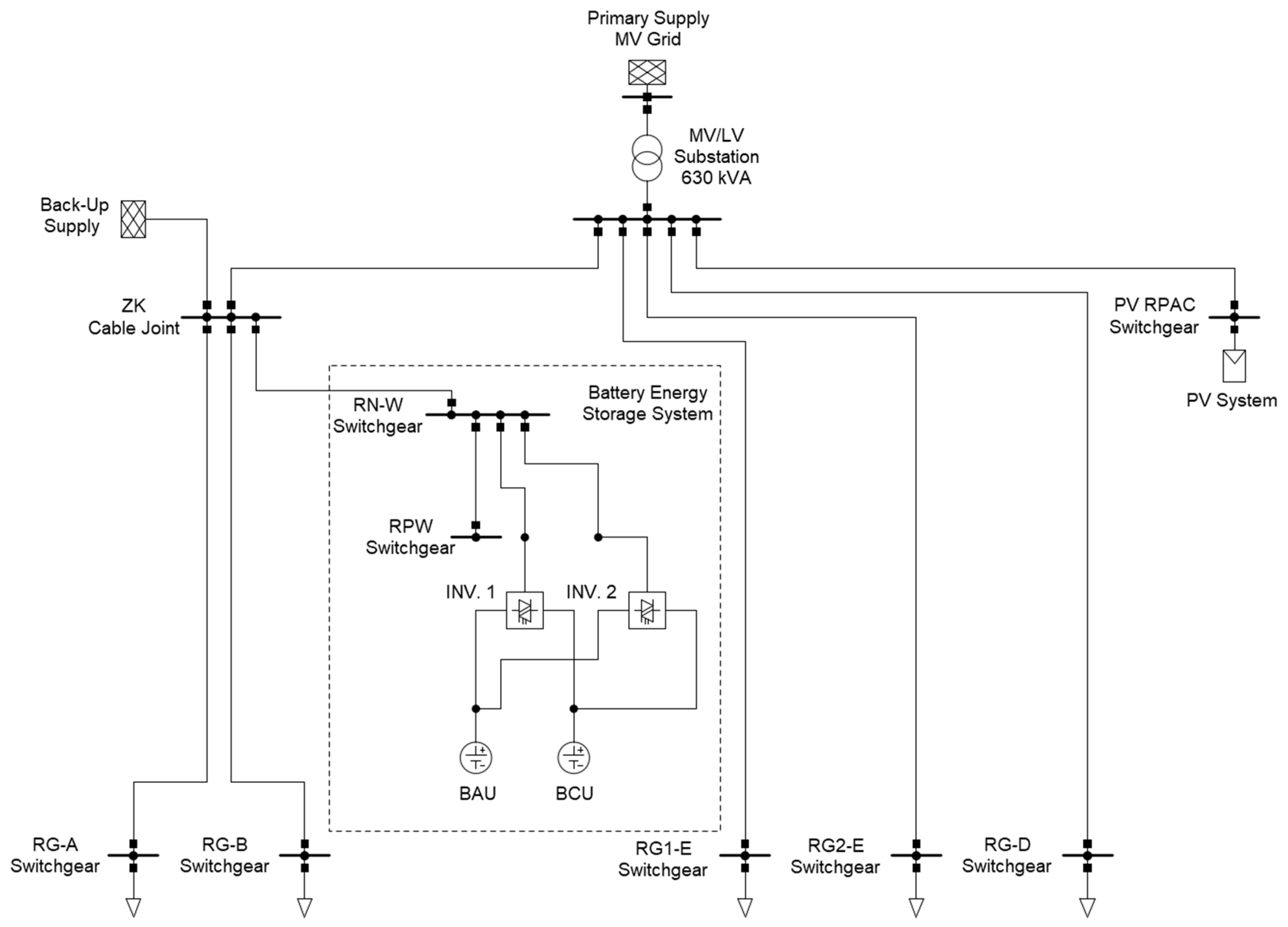
2.1. The Technical Characteristics of the Electric Power Grid in the Considered Factory

Figure 1 presents the connection arrangement of the electric power grid in the considered factory, located on the outskirts of Białystok in north–eastern Poland.
The considered industrial factory is supplied from a grid of 15 kV by means of an MV/LV indoor transformer substation located on the premises of the factory, with a transformer with a rated power of 630 kVA [21,22,23]. A photovoltaic system with a total installed power equal to 317.12 kW (located on the roof of one of the buildings) and the electrical energy battery storage system of 50 kVA rated power and 177.6 kWh rated capacity are also located on the premises of the factory. The MV/LV substation is connected at the LV side (0.4 kV), with some number of switchgears located inside the factory as well as with the mentioned photovoltaic installation and electrical energy storage system [21,22,23].
Located in the building with the electrical energy storage system, the “Inv. 1” inverter (bidirectional converter) of 50 kVA/50 kW with battery packs marked as “BAU” and “BCU” (each one of 88.8 kWh energy) serves as the energy storage system. In turn, the “Inv. 2” inverter (unidirectional converter) of 200 kVA/160 kW together with the “BAU” and “BCU” battery packs creates a UPS system [21,22].
Four industrial laser sets are the leading electricity receivers in the considered factory. The maximum demand for power of the biggest unit was approximately 54 kVA. Each laser acts continuously for 24 h daily and is independent from the others. The lasers cut metal elements [21,22]. The factory’s production profile is described in detail in [21]. A charging station for electric vehicles—EVCS (with maximum power equal to approximately 21 kW)—is supplied, among others, from the “RG-B” switchgear. In turn, an electric heater—EH (with maximum power equal to 4 kW)—is supplied from the “RG-A” switchgear, among others. The electric heater is installed in the domestic hot water tank in the boiler room. The charging station for electric vehicles and the electric heater act as controllable loads [21,22,23].

2.2. Preliminary Analysis of Collected Measurement Data

Selected daily load curves and generation curves in the scope of active and reactive energy, which were prepared based on measurements performed in the considered factory, were characterized [24].
The measurements were performed in April, May, June, and July 2023, on all days of the week. The obtained measurement data were normalized regarding an arbitrarily assumed value of reference. Selected measurement data from the considered days of the week and the mentioned months of the measuring period were analyzed. There were working days (Wednesday), Saturday, Sunday, and holidays. Measurement data were averaged in 15 min intervals [21,22,23].
When analyzing all the curves of the consumption and generation of active and reactive energy for particular months and days of the measuring period, the following conclusions could be drawn [21]:
  • The largest total hypothetical consumption of active energy occurred in different hours of the day; it is worth mentioning that, most often, it took place in the hours of 11:00 a.m.–1:00 p.m.
  • The total hypothetical consumption of active energy on Saturdays was almost always significantly smaller than on Wednesdays, while on Sundays, it was most often a bit smaller than on Saturdays.
  • A considerable daily variability in the total hypothetical active energy consumption was usually observed.
  • The largest total hypothetical consumption of reactive energy occurred at different hours of the day; it is worth mentioning that there was no clear pattern.
  • Charging the energy storage system occurred almost every day; it is worth mentioning that there was no clear pattern observed regarding the hours of the charging process.
  • There were days in which the discharging process of the energy storage system did not occur; if the discharging of the energy storage system occurred, then it took place most often in the evening hours.
  • The amount of electrical energy utilized for charging/discharging the energy storage system on Saturdays and Sundays was most often larger than on Wednesdays.
  • The largest generation of active energy took place in the hours from 11:00 a.m. to 4:00 p.m.; it is worth mentioning that it was most often between 11:30 a.m. and 1:30 p.m.
  • The maximum active energy generated by the PV installation was usually a significant part of the maximum total hypothetical consumption of active energy at the considered factory level, i.e., from around 45% to even 80% of the consumption. Additionally, the amount of active energy generated by the PV installation was usually quite large, large, or very large in relation to the total hypothetical consumption of active energy for the considered factory during the day.
  • A considerable daily variability in the active energy generated by the PV installation was usually observed.
In the case of holidays, the following was observed [21]:
  • The largest total hypothetical consumption of active energy and reactive energy occurred at different hours of the day;
  • The largest total hypothetical consumption of active energy was about 55–60% of the largest total hypothetical consumption of active energy on Wednesday, which was chosen as a reference day;
  • The consumption of reactive energy was much smaller than the consumption of active energy;
  • Periods of charging and discharging the energy storage system did not always happen during these days;
  • The amount of active energy generated by the PV installation during the exploitation hours of the installation was large or quite large, in relation to the total hypothetical consumption of the active energy during the day.
It should be noted that, in all the analyzed curves of the active and reactive energy consumption in the particular months and days of the measuring period, the following relations were observed [21,22,23]:
  • The daily variability in active energy consumption was much larger than the daily variability in reactive energy consumption;
  • The consumption of reactive energy was much smaller than that of active energy.
It should also be noted that, in all the analyzed curves of the reactive energy generation in the particular months and days of the measuring period, the generation of reactive energy by the PV installation was not too large [21,22,23].

2.3. Proposed Preventive Measures for Reducing Peak Electricity Loads at the Level of the Considered Factory

In order to reduce peak electric loads at the level of the considered factory, it was possible to apply the following preventive measures [21,22,23]:
  • Limitation of the levels of power and energy received by power loads exploited in the factory;
  • Shifting the power consumption periods of the power loads exploited in the factory during the day.
Additionally, it was possible to apply the following preventive measures [21,22,23]:
  • Increasing the level of electric power and energy produced by a generation source located on the premises of the factory;
  • Applying appropriate operating regimes for the electric energy storage system located on the factory premises.
As for the possibility of a reduction in the level of power and energy received by power loads exploited in the analyzed factory, it is worth mentioning, in this respect, the general characteristics of the technological processes realized in the considered factory. As a result of these characteristics, most of the observable big power loads were situated in Building “B”. There were four sets of lasers in particular; it is worth noting that each laser acted regardless of the other lasers. As the working conditions show, the possibility of a reduction in the level of power and energy received by the laser sets, due to the often random nature of their work and technological aspects, would not have been easy. Apart from the set of lasers, it is also worth mentioning the controllable loads, i.e., an electric heater located in Building “A” and a charging station for electric vehicles, supplied from the main switchgear, located in Building “B”. In both cases, it was possible to reduce the level of power and energy received by the mentioned devices. It should be recalled, however, that the rated powers of the devices were not very large in relation to the peak demand on the power of the considered factory.
As for the possibility of shifting power consumption periods of the power loads exploited in the considered factory during the day, the same conditions applied here as in the above case. It would have been possible for the electric heater and the charging station of electric vehicles (that is, for controllable loads), while it would not have been easy in the case of the laser sets.
Regarding the possibility of increasing the level of electric power and energy produced by a generation source located on the premises of the considered factory, this would, in practice, result in the need to increase the installed capacity of the existing PV installation or the necessity to build an additional PV installation. It is difficult to assess if this would be an easy task to accomplish in the short term.
Yet another possibility for limiting electric load peaks at the level of the considered factory was applying appropriate operating regimes (charging, discharging) for the existing electric energy storage system. As discussed in [21,22], this preventive measure is a perspective approach. The results of the analysis carried out in the DIEGO project [21,22] indicated that, for each day, it was possible to define the appropriate period for charging and discharging the electrical energy storage system installed in the considered factory. In order to flatten the load at the level of the considered factory, the demand for electrical power and energy would need to be shifted during the day. Thus, the installed storage system can limit the peak daily demand for active energy (reduce the peak active power). It is worth noting that choosing relevant parameters for a functioning energy storage system is an important issue in this context. This issue has been analyzed, e.g., in [25,26,27,28].

2.4. Feasibility and Effectiveness of Proposed Preventive Measures: Analysis Based on Measurement Data Samples

If all the mentioned preventive measures (PMs) were used, they would theoretically decrease the peak electric loads at the level of the considered factory.
In order to evaluate the effectiveness of the defined PMs, simulated calculations on the model of a sample electric power grid were performed [23]. The sample electric power grid had characteristics similar to those of the real electric power arrangement functioning on the industrial factory’s premises. A model of the sample grid was developed in the PowerFactory environment. The model was based on technical data obtained in the inventory process of the real electric power arrangement and measurement data originating from devices installed in outgoing bays of a low-voltage main switchgear, the circuits supplying main electricity loads, the PV installation, and the electrical energy storage system.
The mentioned calculations were performed on a selected working day (on Thursday) in the period from October to November 2023. The following PMs were subjected to simulated verification [23]:
  • PM1—Shifting the demand for electrical power and energy of the laser sets installed in the factory in the range of ±60 min (four periods of 15 min). The time horizon adopted in this study results from the specific technological process in the analyzed industrial facility. In particular, the laser start time could be shifted forward or backward by 15, 30, 45, or 60 min. The laser start-up process is not fully automated and requires the operator’s presence. Moreover, the cutting time depends on the thickness of the processed material. Cutting operations requiring longer processing times are conducted during the day shift, while elements with shorter processing times are handled during the afternoon and night shifts. As a result, the facility owner determined that the permissible time shift for the laser start-up—and consequently, the corresponding power demand adjustment—must not exceed one hour.
  • PM2—An increase of 50% in the capacity of the electrical energy storage system located on the premises of the factory in comparison with the rated capacity of the currently functioning system.
  • PM3—An increase of 50% in the level of electrical power and energy delivered from the PV installation existing on the premises of the factory in comparison with the installed power of the currently operating PV installation.
  • PM4—The modification of the control algorithm for the operation of the electrical energy storage system. The changed control algorithm assumed that the storage system would be charged if and only if a surplus of active power generated over the factory’s total demand for active power took place. In turn, the discharging of the storage system (and in this way, a reduction in the peak power load of the factory) would take place when the value of the active power received from the DSO grid was greater than 100 kW. In the case of power consumption from 0 to 100 kW, the storage system would be switched off. The discharge threshold of the energy storage system was set at 100 kW of power drawn from the distribution grid, reflecting the relatively small capacity of the storage system compared to the facility’s daily energy demand. This setting allows, on the one hand, for a reduction in peak power demand from the grid and, on the other hand, prevents the storage system from discharging too rapidly when recharging from the PV source is not possible.
In the simulated calculations, variants composed of several of the above (basic) preventive measures were also considered (11 such variants from PM5 to PM15) [23]. An explanation of which basic variants made up the composite variants is presented in Table 1.
Additionally, variant PM0, treated as a reference variant, was examined. For the PM0 variant, calculations based only on measurement data obtained from devices located on the premises of the considered factory were performed.
Values of the peak daily load (demand for active power) of the MV/LV transformer substation supplying the analyzed factory in relation to the PM0 variant are shown in Figure 2.
From the performed simulated verification results, a reduction in the peak daily load in the scope of the active power of the MV/LV transformer substation supplying the considered industrial factory was obtained in most of the analyzed variants. Variant PM2 was the only variant for which an active power level decrease received from the DSO grid was not achieved. The reductions in the peak daily load for variants PM1, PM3, and PM4 in comparison with the reference variant PM0 were equal, respectively, to 0.05%, 3.08%, and 6.05% [23].
The analysis of the variants combining at least two basic preventive measures results showed that the biggest potential for reduction in the peak daily demand for active power at the level of the considered industrial factory was the variant PM4 and its combination with the variant PM3. The greatest degree of peak daily load reduction (9.12%), compared with the variant PM0, was obtained for the variants PM13 and PM15 (in which the basic variants PM3 and PM4 appeared) [23]. Additionally, the implementation of the variant PM4, consisting of a change in operation algorithm of the energy storage system controller is a low-cost solution. However, it should be noted that the results presented in [23] concern only one day per year.
From the simulated calculations performed [23], it can be stated that applying the defined preventive measures (excluding the variant PM2) in the scope of a reduction in the peak daily load (demand for active power) at the level of the considered factory would be justified.
After analyzing the results of the simulation studies evaluating the effectiveness of the defined preventive measures, consultations were conducted with an industrial partner to discuss the possibilities of implementing our recommended methods for reducing the peak power demand of the industrial plant. As a result, we decided to increase the energy storage system capacity by 50% and modify its operation schedule for the next research phase. The revised operation schedule of the energy storage system is described in Section 2.6, while the results of its operation, considering the latest measurement data, are presented in Section 3.

2.5. Setting the Proper Operating Regimes for Electrical Devices

One of the aims of setting the proper operating regimes for electrical devices was an improvement in the energy efficiency of selected technological processes realized in the considered factory in the scope of electrical energy [21].
The following issues were analyzed in the considered factory within the DIEGO project [21]:
  • A reduction in network losses resulting from reactive energy consumption by various kinds of electrical energy receivers;
  • A reduction in network losses connected with the transmission or distribution of electrical energy, also including losses in the internal distribution systems of electrical energy powering the installations used in industrial processes.
As for the reduction in electrical power and energy losses resulting from reactive energy consumption by various kinds of electrical energy receivers, decreasing the reactive powers drawn by selected electrical energy receivers should be considered as a preventive measure if this is technically and technologically possible [21].
Assuming that the active power P, the resistance R, and the voltage U are constant, active power losses depend on the power factor tanϕ as a square function. Thus, to minimize power losses (and consequently energy losses), efforts should be made to minimize the tanϕ power factor, i.e., to reduce reactive power consumption. This problem requires detailed considerations regarding reactive power consumption in particular production processes carried out in the considered factory. Selected curves of the tanϕ power factor and reactive energy consumption and generation values were characterized in [21]. They were prepared based on measurements performed in the considered factory [24]. All the measurement data obtained for the consumption and generation of reactive energy were normalized against an arbitrary reference value.
The following should be stated [21]:
  • Problems regarding reactive power (energy), both at the level of the entire considered factory and at the level of individual bays supplying switchgears, from which, in turn, devices carrying out specific technological processes are powered, occur. There are 15 min time intervals when the value of the tanϕ power factor exceeds the permissible value of the factor, equal to 0.4.
  • There are also 15 min intervals in which reactive energy is delivered to the grid.
Similar situations occur in circuits (bays) supplying the PV installation, the electrical energy storage system, and the inverter operated as a UPS system [21].
Regarding the reduction in network losses related to the transmission or distribution of electrical energy, also including losses in the internal distribution systems of electrical energy powering the installations used in industrial processes, the aim should be to minimize active power consumption if this is technically and technologically possible. Assuming that the resistance R, the voltage U, and the power factor cosϕ are constant, the active power losses depend on active power P as a square function. In turn, assuming that the electrical energy required in a given cycle of technological process is constant, in order to minimize power losses (and consequently energy losses), efforts should be made to flatten out power consumption profiles (i.e., to reduce the peaks of the occurring loads) [21]. This issue was presented above.
After conducting consultations with the industrial partner, we decided to implement the ability to regulate the tanϕ power factor for the next research phase by changing the reactive power operating points of the photovoltaic inverters and the inverter within the energy storage system. The algorithm for determining the new operating points of the inverters is described in Section 2.6, while the results of its operation, considering the latest measurement data, are presented in Section 3.

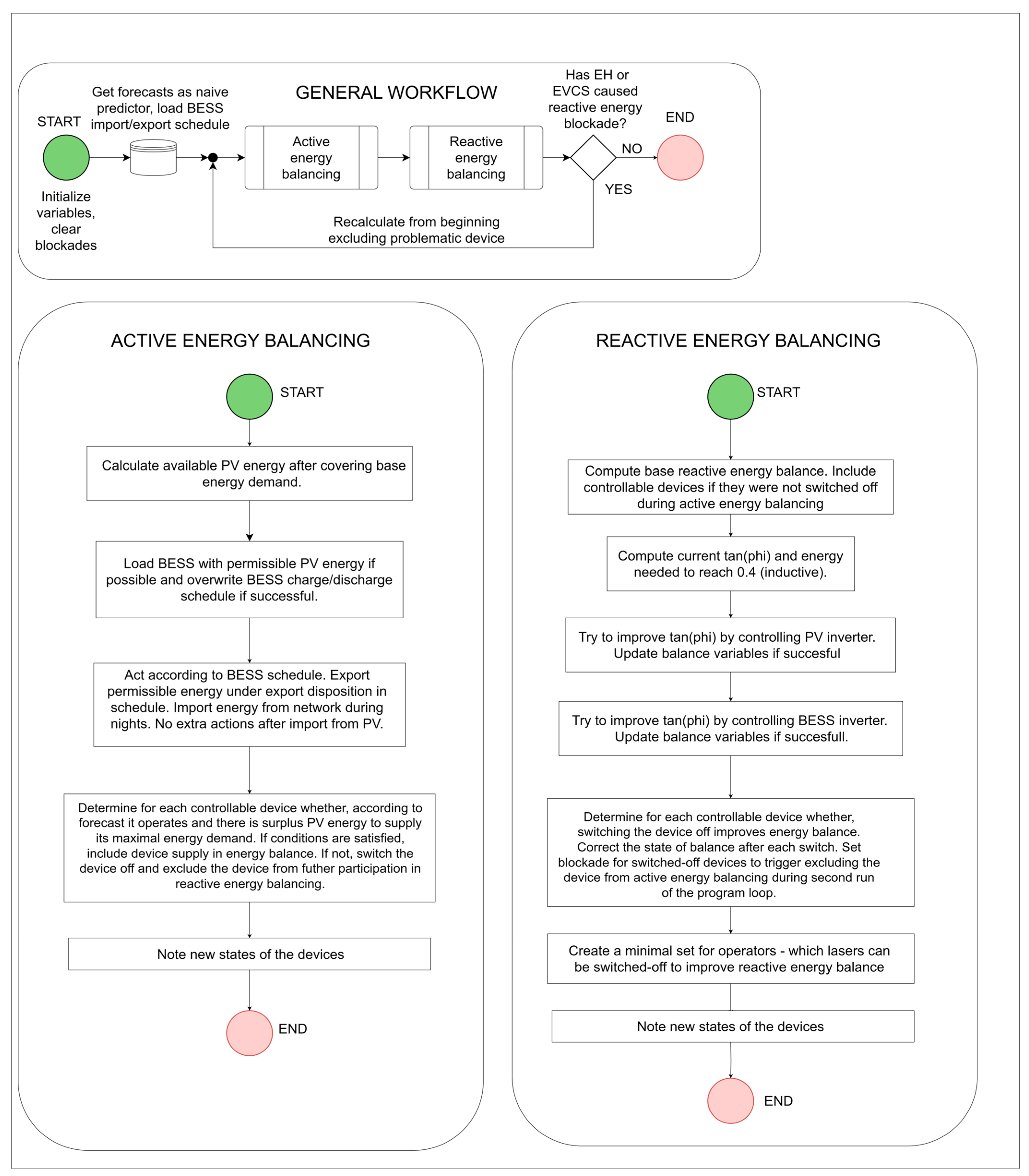
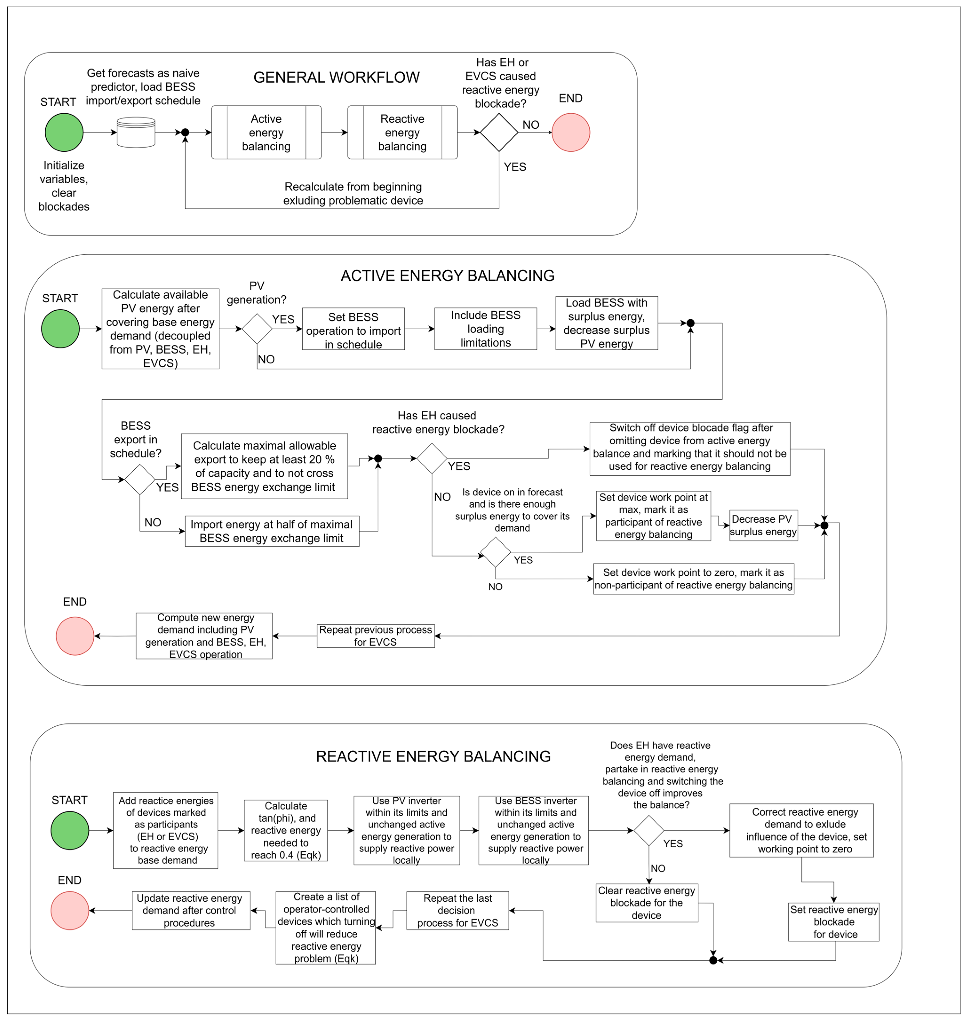
2.6. Control Algorithm Used for Industrial Plant’s Performance Improvement

2.6.1. Introduction

The assumptions relating to the control algorithm were as follows. The goal of operation improvement was to obtain a new, better operation state of the industrial plant for the next 15 min period. Only a scenario concerning 1-step-ahead calculations with a 15 min resolution was considered due to multiple input variables being highly random, which would have a strong impact on their forecastability over longer time horizons.
In the research, several component goals were set. The first of them was decreasing peak electricity demand, and the second was increasing the energy effectiveness of the considered plant. For the latter, the autoconsumption of electrical energy from the PV installation and energy savings were thus to be monitored. The third goal, in turn, concerned enhancing reactive power management. For that purpose, reactive power had to be kept within proper limits, and the phase angle tangent at the main switchgear level had to be monitored.
Our calculations had to use a naive predictor (last known state) as a method of future state estimation prior to the improvement of operation. This method was used mainly due to limited data availability. Amassing data in only the first half of the year 2024 imposed real challenges on the creation of models. On the one hand, to properly reflect the seasonality and periodicity of processes, at least one year of measurement should be used to train and validate newly created prediction models. Moreover, one more data year should be used to check the generalization capability of models. On the other hand, the division of one year of data into training, validation, and test datasets should allow for the mitigation of information leakage that occurs when datasets with periods adjacent to training datasets are used for testing purposes. The above problems could not be addressed with our limited range of obtained samples. Additionally, the behavior of some devices, like the electric heater and electric vehicle charging station, but also the lasers, was too random to create more accurate prediction models with our limited data. The limited forecastability of the mentioned devices required extensive research to overcome a naive predictor. From a potential investor perspective, this extra work could be treated as a potential liability for the entire solution application. As such, the naive predictor constituted a simple, practical solution within our limited possibilities. In the future, however, more accurate methods could be implemented in its place. The powers and corresponding energies of the BESS, EVCS, EH, lasers, PV, MS (main switchgear), and “SG1” (bay no.1 in the main switchgear, supplying a cable joint “ZK”, from which in turn the “RG-A” switchgear and the “RG-B” switchgear are supplied) were all forecasted with the naive predictor as the initial conditions of operation improvement.
Device work characteristics and their consequent limitations were further considered in operation improvement. The lasers were assumed to be non-controllable devices due to their typical real-life use. The BESS, in turn, had two types of limitations. The device needed to operate within 20–100% of its capacity, while the active energy exchanged within a 15 min period should not exceed the maximum energy allowed by the inverter (12.5 kWh). To properly satisfy the first BESS limitation, the state of charge and exchanged energy had to be updated after each run of the improvement procedure. The next pieces of equipment to be included in the calculations were the inverters of the PV system and BESS, which introduced constraints on reactive energy under a given level of active energy. Other general requirements imposed additional limits on allowable powers. The power of the devices had to be kept within their minimum and maximum ranges.
In the considered scenario, the EVCS and EH were treated as controllable devices. Due to their highly random characters of use, and thus the practical difficulties with highly accurate forecasts of their use, only two possible states of operation were assumed for the devices—work at their rated power or no operation at all. Those devices were turned on only if, according to forecasts, they would operate, and there would be a surplus of generation covering at least a given device’s maximal demand after the PV system fed the entire plant’s demand.
Various assumptions had to be made for potentially effective reactive energy management. If this energy was capacitive, the algorithm had to decrease it through the control of the PV system and BESS’s inverters. If it was inductive, the algorithm had to try to decrease its value only if the phase angle tangent exceeded 0.4. The decrease in inductive energy had to start with PV and BESS inverter control. Next, but only if it helped to reduce the problem, controllable devices would be turned off. After that, a list of lasers to be turned off was created, starting with lasers with the greatest inductive energy demand. A similar process was constructed for capacitive energy. Since the potential cost of turning the lasers off at a given time was hard to predict, the list showed only propositions, and no turning off happened in the program for lasers. In real-life use, the decision to accept turning off has to be individually made by either the owner or the laser operator, which was hard to imitate during the simulations phase.
Since one of the improvement procedure goals was to reduce peak load demand, planning the operation of the BESS was used as a means to an end. The BESS had an operation schedule that could be overwritten during the program run. According to this schedule, the BESS was discharged between 08:00 and 18:00 with a 15 min time resolution, and it charged during the rest of the day. The schedule was overwritten with charging from the PV system if there was a surplus of generation above the industrial plant’s demand. If the BESS was already full, the algorithm tried to supply energy to the electric heater or EV charging station. Obviously, when the EH or EVCS were turned off due to reactive energy problems, the entire energy balance was recalculated to exclude them from both the active and reactive energy demand.

2.6.2. Generic Workflow of Algorithm

Initially, the program loads data and inserts them into corresponding data structures. At this stage, the primary state of operations is loaded for the industrial plant (among which is the plant’s electricity demand before the improvement procedure). Next, the balancing happens. First active energy is balanced, and then reactive energy. During balancing, the program iterates over devices—the PV system, BESS, EH, EVCS, lasers, and network. The order of device appearance in calculations is dependent on settable prices, which allows the model to imitate energy auctions. During its operation, the program determines new operation states for devices, which facilitates, e.g., calculating energy effectiveness metrics by comparing new states with old ones.

2.6.3. Active Energy Balancing

First, the program determines whether there is a surplus of PV generation over the industrial plant’s active energy demand. If the condition is met, the algorithm tries to charge the BESS. On success, BESS is charged within permissible constraints; its state of charge, exchanged energy, and charge timetable are overwritten. The surplus is also reduced. Next, the program tries to supply electric heater or charging station of EV. If, according to the forecast, they would operate and the existing surplus can cover their maximal energy needs, they are supplied and included in the reactive energy balance.
Next, the BESS inverter is checked. If the BESS should be discharged according to the timetable, the program determines discretionary energy according to discharge limitations. Energy is discharged gradually to facilitate peak demand reduction for multiple time periods. If the BESS should be charged instead (and it did not happen with PV help), the energy is taken from the network. The taken energy value is equal to half of the maximal chargeable energy in order to achieve potential charging from the PV system in the next time period.
As described previously, controllable devices are considered by the algorithm next. If, according to the forecast, the devices operate, and there is surplus PV generation that is able to cover their demand, they are supplied in reactive energy balancing. If the surplus value is too low, or the devices operated but were blocked from operation during the reactive power balancing stage, the devices are determined to be turned off. This operation is followed by setting the switched-off controllable device as not participating in reactive energy balancing.
The last step of active energy balancing is checking whether a surplus of PV generation still exists after all the device feeding trials. For this unlikely situation, the program controls the PV inverter to make the surplus 0. Eventually, the rest of the demand (if it is not covered entirely by the PV system) is determined as energy taken from the grid.
The simplified active energy balancing procedure comes down to 3 main stages. During the first one, the decision is made whether the BESS should be loaded with PV energy. If this happens, the program charges the BESS within permissible limits and overwrites a predetermined charge/discharge schedule for the BESS, which is the basis for the next stage. During the second stage, the program checks whether the BESS should import or export energy according to its operation schedule. For exporting, the state of charge and operational limits are included to find how much energy the BESS can export. If, however, the BESS has to import energy (in a situation without PV production or at night), an additional condition is imposed on the transfer limit to allow the BESS to potentially import free PV energy during the next period. The third stage of active energy balancing concerns trying to supply controllable loads if they operate (according to forecast) and there is surplus PV energy to supply them. If satisfying those conditions is impossible, the devices are set to switched-off and not included in reactive energy balancing. The fourth (minor in this case) stage concerns, in turn, noting the new states of the devices.

2.6.4. Reactive Energy Compensation

For reactive power, the first step is to add the reactive power demand of the controlled devices if they were previously specified as turned-on. Then, the program calculates the new demand for active and reactive power by adding the previously specified new active power of the devices and the existing reactive power. Based on this, whether the plant’s resultant reactive power demand is capacitive or inductive is further determined.
For inductive demand, the energy that needs to be reduced to achieve a power factor tangent of 0.4 is determined. If this energy is negative, the operating state remains unchanged. However, if this energy is positive, an attempt is made to control the photovoltaic inverters and the energy storage system to maximize the reduction in reactive power consumption. Subsequently, it is checked whether turning off the controlled device will reduce the reactive power demand.
If the device has a reactive power demand, and doing so would improve the situation, the device is turned off, and a blockade is set for this device due to the reactive power. Subsequently, this lock causes the program to recalculate the energy balance, this time without including this device in the balance.
In the case of capacitive energy, an attempt is only made to control the inverters to increase the import of inductive reactive energy. In case of further problems, with both inductive and capacitive power, it is determined which lasers should be turned off to get as close as possible to solving the problem. The program’s operation scheme is shown in the block diagram in Figure 3. To allow the reader to track each operation as a more general flow, we additionally present a simplified flowchart in Appendix B.
The beginning of reactive energy balancing stays the same for both types of reactive energy demand. The program tries first to control the inverter of the PV system within permissible limits to mitigate the problem, accounting for the active energy needed for active energy demand. Then, it tries to do the same with the energy storage inverter. Only after that does the program check whether the character of the reactive energy demand is still capacitive, after the potential operation of source and energy storage inverters. Then, the program checks whether controllable device load shedding would improve total reactive energy balance.
In the presented case, the controllable devices included only the electric heater and EV charging station, but the entire operation scheme was planned to be generally applicable. Hence, if reactive energy demand was negative after the inverter operation stage, the program went through each controllable device (sorted from least to most important for user convenience) and checked whether switching off a given device helps mitigate the problem. If not, no change in state occurs so as not to worsen the problem. For the opposite situation, the switching happens, the Eqk value is adjusted, and a device blockade is set due to the reactive energy problem. This way, it is possible to switch on/off a minimal necessary number of elements. A similar operation scheme is applied to inductive reactive energy demand. For this situation, the program iterates over devices, checks whether switching them off would reduce the problem, adjusts Eqk after each switching, and sets device-specific reactive energy blockades. Since, for both signs of Eqk, the applied methodology is the same (with of course accounting for the proper signs of energies), in the diagram both cases are presented as one.
To allow the program to account for the fact that some devices may have been switched off during the reactive balancing stage, in case a reactive energy blockade was confirmed after the reactive balancing stage, the program goes back to the active energy balancing stage to exclude the active energy of the blocked devices from balancing and clear blockade flags.
One may observe that an arbitrary decision was made to first use inverter control instead of using load shedding first. This was caused by the assumed priorities of operation, meaning that if there is a surplus of active energy that allows for the user-convenient use of controllable devices and increased autoconsumption of own active energy (and, as a result, less energy taken from the grid), this sort of operation should have priority.

2.6.5. Calculation of Algorithm Effectiveness Metrics

After the energy balancing was completed, the quality indicators of the algorithm’s performance were calculated. These included the plant’s self-consumption of energy from photovoltaics, the new power factor tangent, and industrial plant electricity demand after control operation.
The saved energy can be expressed by the Formula (1):
s E t = E t b e f E t a f t
where
  • t—type of energy, p for active energy and q for reactive energy.
  • bef—state before control of industrial plant took action.
  • aft—state after control.
  • s E t —saved energy, with unit dependent on type of energy.
It should be noted that E t b e f and E t a f t are both given the “observable” label in the algorithm code. This means that they should be interpreted as values observable directly at the main switchgear meter level. This distinction is important because the observable demand at this level was deconstructed prior to the calculations to find the industrial plant’s “raw” demand (one without the influence of PV and energy storage). This allowed for the creation of a “purer”, more robust time series for our forecasting needs. However, to compare the values in a way that can replicate real-world measurement, after control operations calculations, we had to add the factors that were previously eliminated to obtain a state of variables comparable in a physical sense to the measurements.
The autoconsumption of PV energy can be expressed by the Formula (2):
S A C E t = P V E t E t i f   E t 0 N o n e i f   E t = 0
where
  • t—type of energy, p for active energy and q for reactive energy.
  • S A C E t [ ] —autoconsumption degree of a given type of energy generated by the industrial plant’s PV system.
  • P V E t —a given type of energy generated by PV.
  • E t —t-type energy demand, directly corresponding to either E t a f t or E t b e f .
t a n φ can be expressed by the Formula (3):
t a n φ = Q P = k · E q k · E p = E q E p i f   E p 0 N o n e i f   E p = 0
where
  • k 0 —a constant allowing us to create equivalent power corresponding to the given energy at the end of a considered 15 min period.
  • E p —the active energy measured in the considered 15 min period.
  • E q —the reactive energy measured in the considered 15 min period.
Again, this metric was calculated for states both before and after control took action, and the energies here refer to observable values.
When shown, the metrics allowed us to rate the momentary quality of the given solution. Unfortunately, some operations logic, such as moving the peak of electricity demand to demand valleys, can be inherently characterized by a momentary decrease in metrics to achieve better total results for longer periods of time. As such, to show a more general image of the data behavior before and after the control operations, metric distribution was additionally computed and is presented in Appendix A. Please note that, in Appendix A, deltas (change between state before and after control operations) are also calculated for metrics in order to give the reader an idea of how much the distribution of the variables changed after control operations. Additionally, compared to Appendix A, some outliers had to be filtered out to achieve a properly wide scale of the diagrams in the main text.

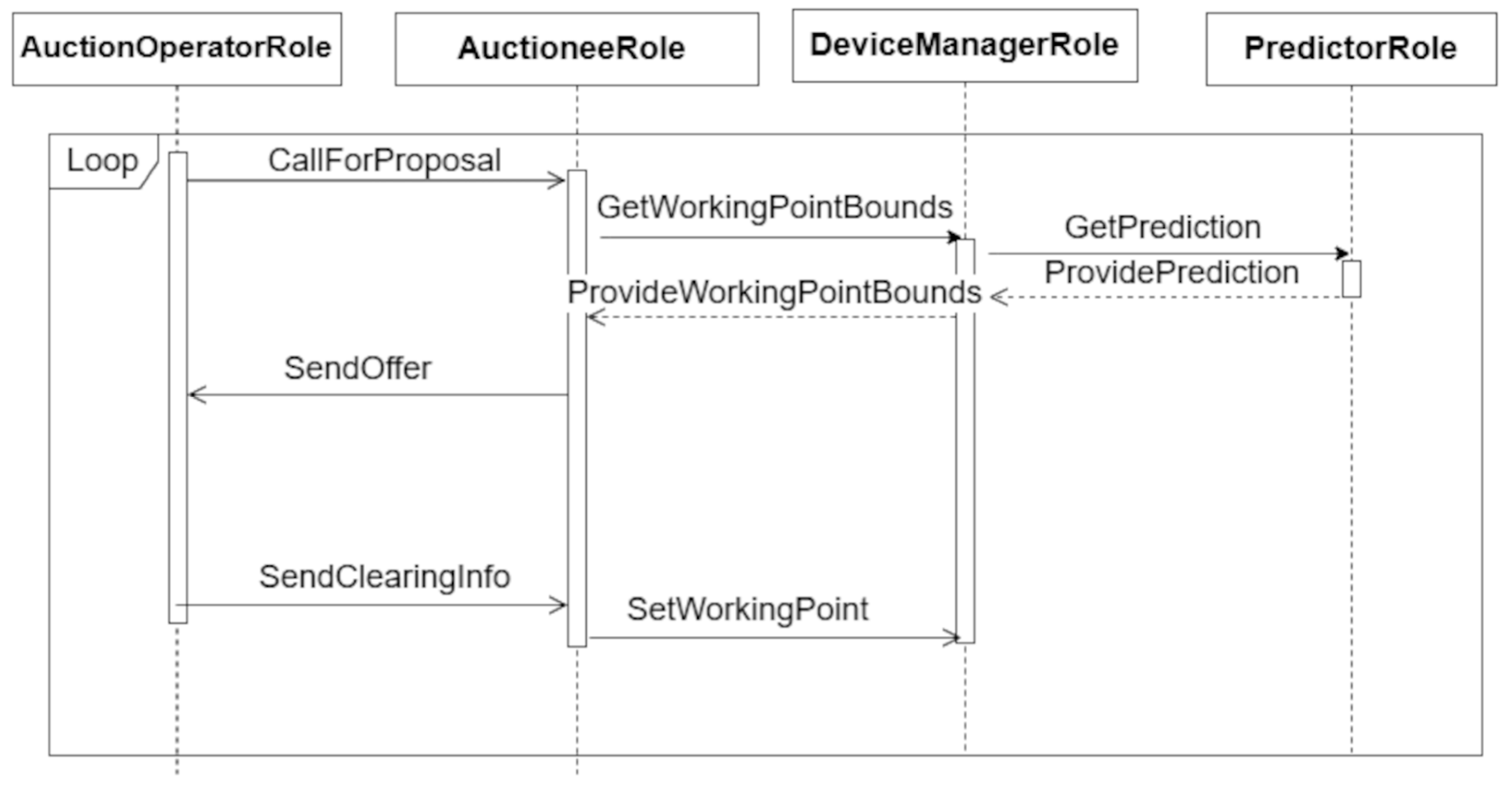
2.7. Multi-Agent Systems for Reducing the Peak Power Demand and Setting the Proper Operation Regimes of Electrical Devices Located in the Factory

We propose using multi-agent system technology to implement the dynamic energy management in an industrial facility. A MAS would optimize active energy balancing and reactive power compensation through a centralized bilateral auction mechanism, executed in 15 min intervals. The autonomous agents represent controllable and non-controllable devices, coordinating to ensure efficient energy use while complying with grid requirements.
A multi-agent system is a system where a number of autonomous software entities (agents) exist. Every agent has its own specific goal and information, and to reach the goal, it should interact with the other agents [29,30]. In the described problem, energy balancing in industrial plants requires real-time coordination between multiple entities (consumers, sources, storage).
The representation of devices by agents assumes the existence of agents representing each device, taking care of their characteristics. The predictions for every device are handled by a special predictor agent. We assumed the representation of non-controllable devices (i.e., those for which it is not possible to influence the current level of energy consumption/production) and controllable devices, i.e., those for which it is possible to control the level of energy production or consumption partially or entirely. These agents submit bids for the next 15 min, both for active and reactive power. The bids are collected by the auction operator, which performs the balancing procedure. Energy balancing in the considered facility was performed as a centralized double auction, which was carried out by “AuctionOperatorRole” every specified time period (15 min). The active energy in the balancing window was calculated as the sum of the energy measured in all three phases at the connection point to the DSO distribution network. As the energy balancing is performed using the double auction, the offers submitted are differentiated using prices. The higher the bid price and the more advantageous it is for the auction operator (i.e., the lower the sale price and the higher the purchase price of energy), the higher the priority of the given bid. In case the conflict is not resolved, the algorithm used for the balancing process, described in detail in Section 2.6, decides.
The main functional requirements (FRs) for a MAS used to balance electricity in real time and establish appropriate operating regimes of devices located in the considered industrial plant can be summarized as follows: balance active energy (FR1) and compensate reactive power (FR2); operate at the grid connection point (FR3) via agent collaboration (FR4); access real-time device parameters (FR5–FR7) and 15 min forecasts (FR8); and execute auctions for active (FR9) and reactive (FR10) energy every 15 min. A more detailed description of the system is described in [22].
From the requirements set, the project of the multi-agent system was created according to the GAIA [31] methodology for the design of the multi-agent system. We distinguished the following roles [22]:
  • “AuctionOperatorRole”, whose purpose was to organize the double auctions between participants represented by “AuctioneeRole”, clearing and sending the results back to participants.
  • “AuctioneeRole”, the purpose of which was to report a bid to buy (to consume energy from a specified range or, in the case of rigid bid, a certain amount of energy) and a bid to sell (to deliver energy from a specified range or, in the case of rigid bid, a certain amount of energy) to the “AuctionOperatorRole” role. The type of bid and the purpose for the specific type of energy (active or reactive) were specified in the data. This role received information about the device (current operating point) from the “DeviceManagerRole”. After receiving a decision from “AuctionOperatorRole” regarding the established operating point of the device, it passed it to “DeviceManagerRole”.
  • “DeviceManagerRole”, whose purpose was to transfer data from the device (current operating point, permissible operating range) and predictions (working point prediction, working range prediction) to “AuctioneeRole”, setting the current operating point resulting from the auction. The requests for predictions were sent to the appropriate “PredictorRole”.
  • “PredictorRole”, which calculated the prediction for the operating point or operating range of the appropriate device. It received the request, calculated it, and sent it back to “DeviceManagerRole”.
The flow of communication in a single process of balancing is presented in Figure 4.
Delays in message transmission are a natural phenomenon considered in the implementation of multi-agent systems, and the platforms used for their implementation propose technical solutions based primarily on the recipients of messages waiting for them to be received. On the other hand, waiting too long for a message can lead to blocking the system’s operation. Therefore, a good solution that has been used is to wait for a response for a minute (with a repeatability period of 15 min). Such a long waiting time (with a typical exchange of messages in an order of several seconds) is sufficient.
The multi-agent system was implemented in SPADE (Smart Python Agent Development Environment) [19,20]. Communication among agents was performed through the XMPP protocol [32], and the Tigase implementation of the XMPP server was used [33]. To ensure the portability of the solution, it was placed on two docker [34] instances: the multi-agent system on one docker and the Tigase XMPP server on the second docker. The multi-agent system implementation could be split into particular groups of agents, with each exemplary group representing the devices, and those groups could be placed into separate dockers.
The implemented solution concerned 17 agents that represent physical devices (PV system, BESS inverters, lasers, EH, and EVCS), power supply points (individual bays of MSs and external networks), and states of charge (SOC) of BESS. Each of such agent was represented by a group of three (sub)agents: “Predictor” (implements the “PredictorRole”), “DeviceManager” (implements the “DeviceManagerRole”) and “Auctionee” (implements “AuctioneeRole”). A single “AuctionOperator” agent (implementing “AuctionOperatorRole”) was responsible for setting out the auction every 15 min and sending the “CallForProposal” message to every “Auctionee” agent. The communication language used was JSON, and it put the timestamp to distinguish the specific timeslot. After that, each “AuctionOperator” agent waited for the answer from the appropriate “Auctionee” agent.
After receiving the “CallForProposal” message, each “Auctionee” agent prepared the offer to send back to the “AuctionOperator”. To do so, the “Auctioneer” sent a “Query” message to the appropriate “DeviceManager” agent. The communication language was JSON and the message was composed of the timestamp. Then, each “DeviceManager” waited for the answer.
Each “DeviceManager” agent, after receiving the “Query” message, prepared the details of the device (operating bounds for active and reactive energy, information on whether the device is controllable or non-controllable for active and reactive energy, respectively), and queries the “Predictor” agent for the prediction of, respectively, the active and reactive energy working point or working range.
After that, the agents sent the information back to the requestor, and finally, the “AuctionOperator”, after receiving a whole set of information from every “Auctionee”, processed the balancing procedure. After that, the “AuctionOperator” agent sent the informing communication to every “Auctionee” agent, which contained the clearing info. After that, selected “Auctionees” sent communications to the appropriate “DeviceManager” with instructions to set the working points (both in active and reactive power) to the calculated values.

3. Results

In this section, selected results from the operation of the developed control algorithms are presented.

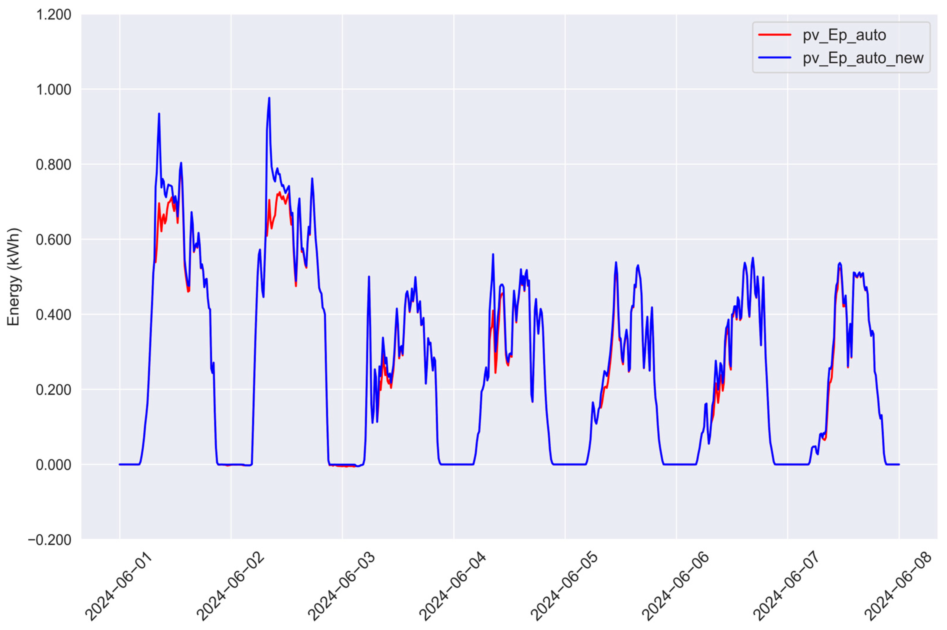
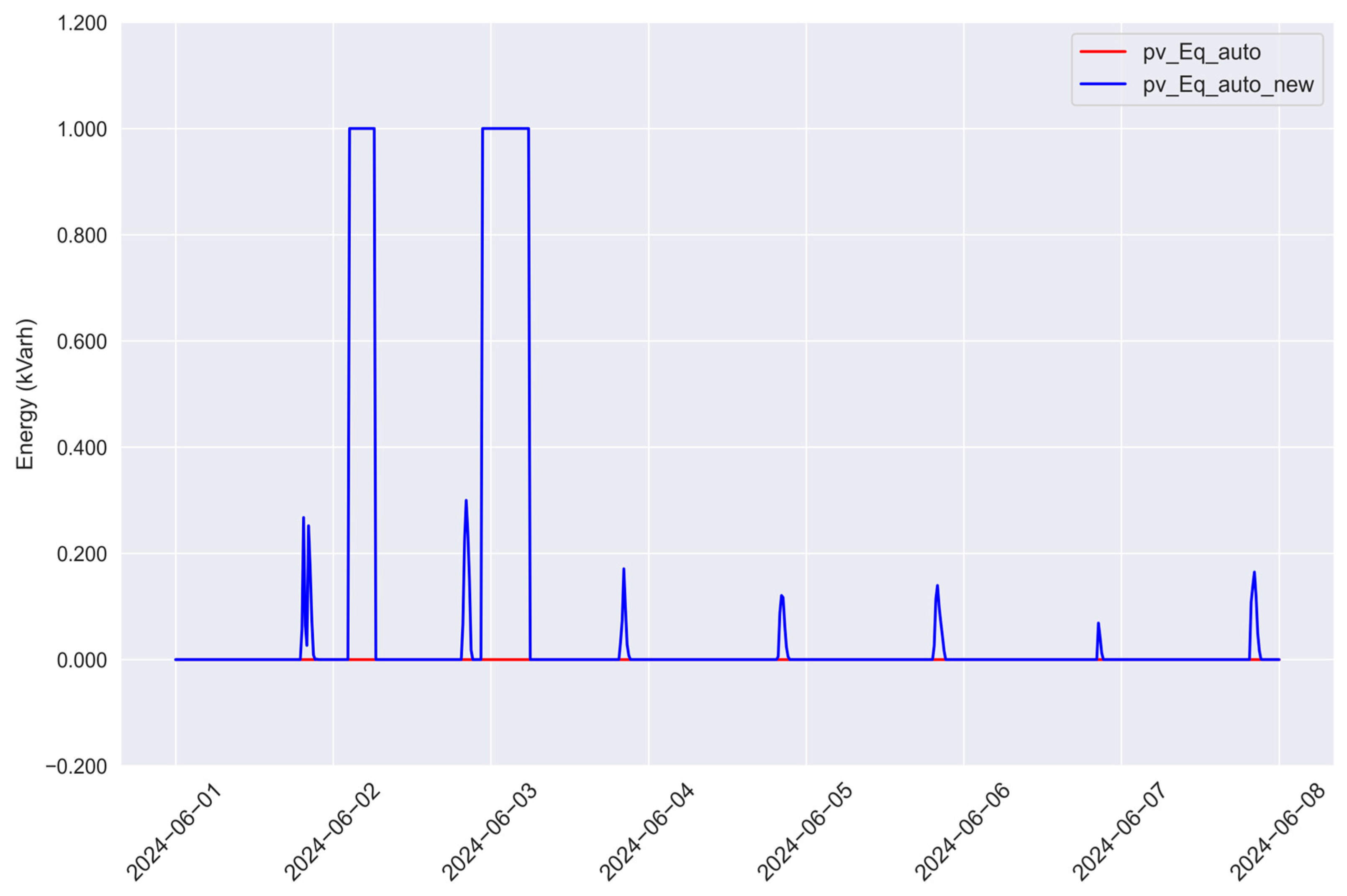
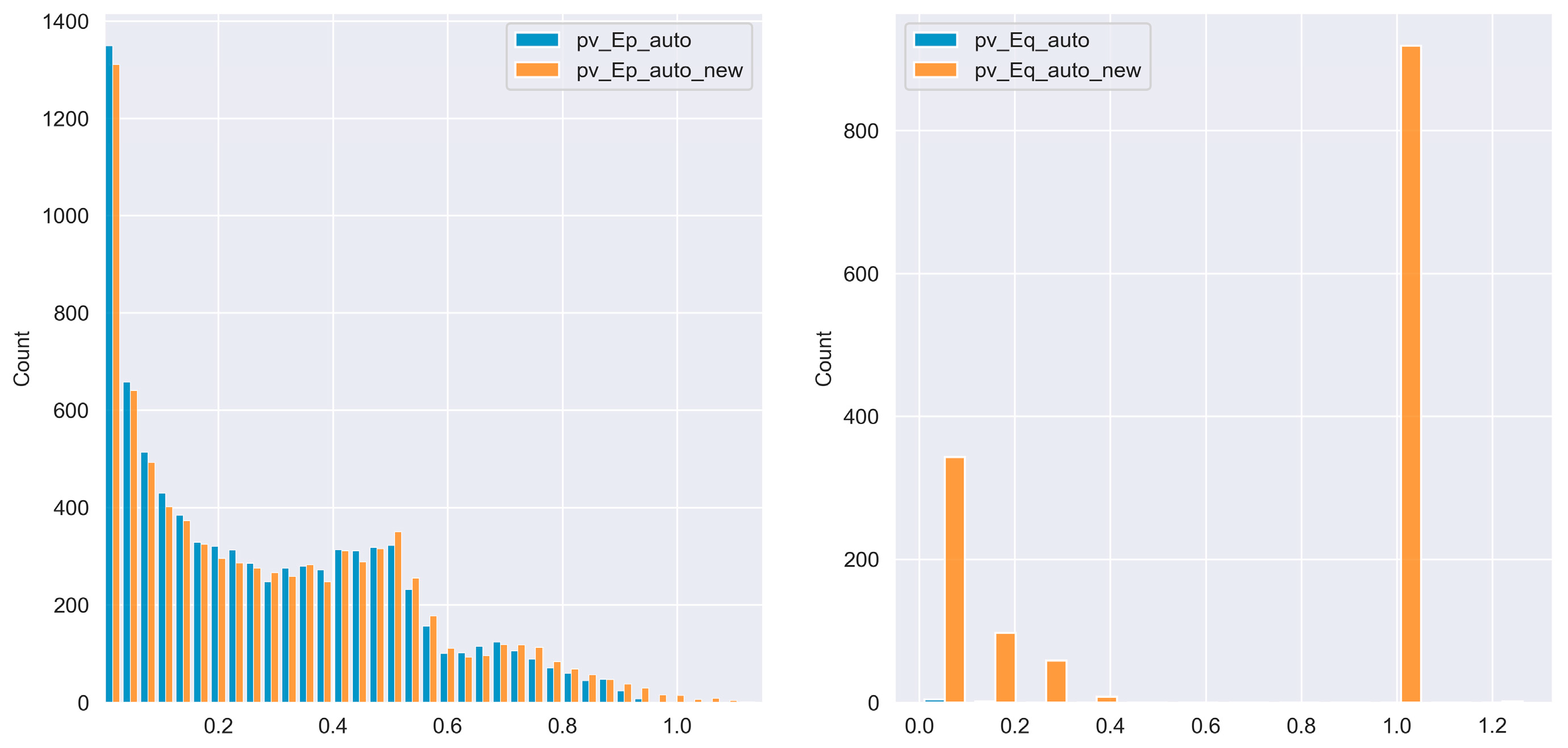
3.1. Statistical Description of Results

As the first step of results analysis, the statistical description of the energy efficiency metrics time series is given. To compare the effectiveness of industrial plant operation before and after the improvement procedure, both the primary state and state after improvement are presented, with respect to active (Ep suffix) and reactive energy (Eq suffix). The considered metrics contained the following:
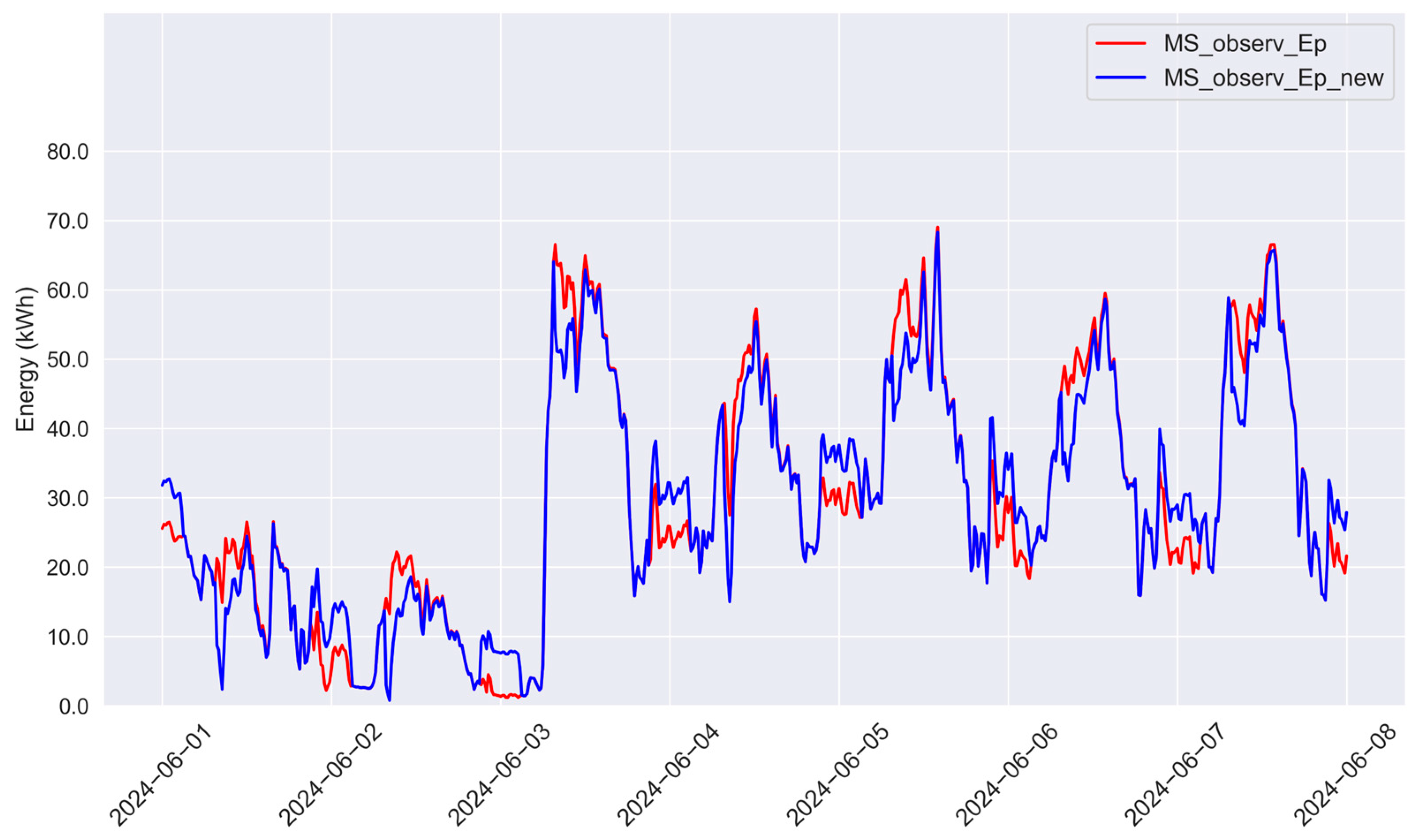
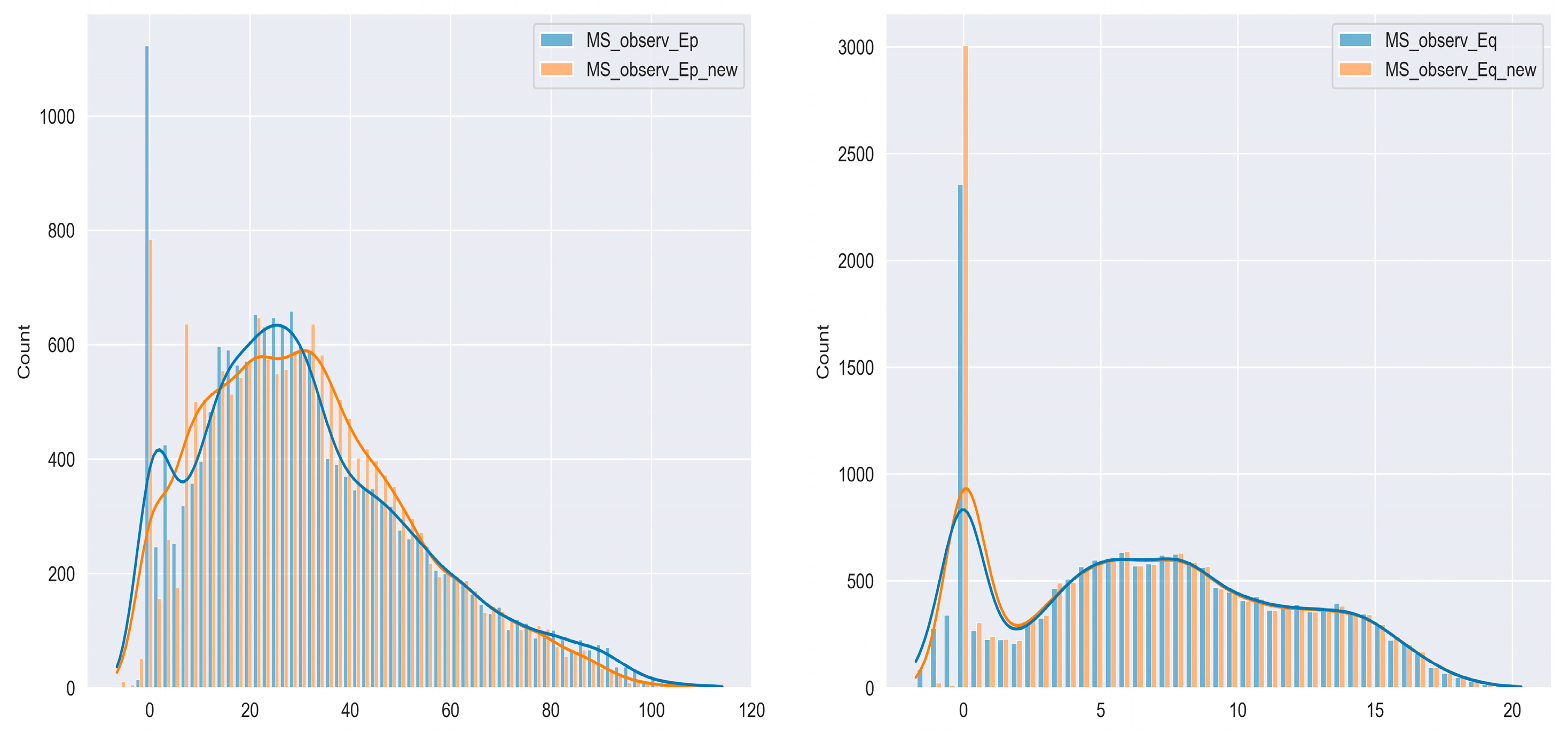
  • Observable energies before the improvement procedure, as seen on the main switchgear level (MS_observ);
  • Observable energies as seen on the main switchgear level after improvement (MS_observ_new);
  • The difference between the observable energies before and after the improvement procedure (delta_MS_observ);
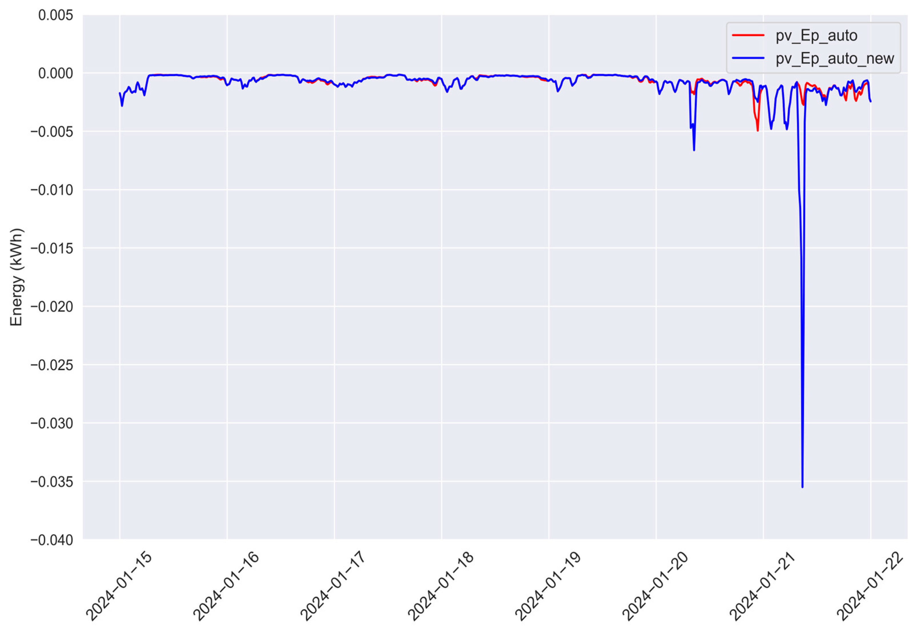
  • PV energy autoconsumption before the improvement procedure (suffix: auto);
  • PV energy autoconsumption after the improvement procedure (suffix: auto_new);
  • The difference between PV energy autoconsumption before and after the improvement procedure (suffix: auto; prefix: pv);
  • The phase angle tangent corresponding to the observable energies before the improvement procedure (tg);
  • The phase angle tangent corresponding to the observable energies after the improvement procedure (tg_new);
  • The difference between the phase angle tangents corresponding to the observable energies before and after the improvement procedure (delta_tg).
The results are presented in Appendix A due to the stats table’s size.
Statistical description allowed us to identify outlier values in some analyzed metrics. Examples of those can be found in the columns pv_Ep_auto_new and tg_new. After looking into the details, it can be noticed that outliers appeared for a minuscule number of the samples (approx. 0.1%). For ease of analysis, the effective range of each variable’s delta (differences between states prior to and after the improvement procedure) was conditionally formatted. For a better illustration, one winter week (15 January 2024–21 January 2024) and one summer week (1 June 2024–7 June 2024) are shown in the figures. Observable active energy and observable reactive energy for the winter period are presented in Figure 5 and Figure 6 respectively. The same variables for the summer period are presented in Figure 7 and Figure 8. The statistical distribution of the observable active and reactive energies before and after the control operation is presented in Figure 9. The autoconsumption of photovoltaic panels’ active and reactive energy for the winter period are shown in Figure 10 and Figure 11, and values for the summer period are shown in Figure 12 and Figure 13. The statistical distributions of PV energy autoconsumption prior to and after the operation improvement procedure are shown in Figure 14 and Figure 15. Tangent values before and after the operation improvement procedure are, in turn, shown in Figure 16 and Figure 17. The statistical distributions of tangent values prior to and after the operation improvement procedure are shown in Figure 18.
A first look at Figure 5, Figure 6, Figure 7 and Figure 8 confirms the effectiveness of the improvement procedure for demand peak shifting. The effect was observable for active energy; the peaks were shifted to night hours, thus achieving the declared energy saving. For reactive energy, in turn, the states of operation were mostly similar, which can be attributed to non-controllable devices like lasers being the main reactive energy consumers. The observable effect in this case mostly shows the proposed solution’s ability to deal with states of capacitive power consumption effectively.
Analyzing percentiles of the entire time series of observable active energy, it can be seen that an improvement of 5 up to approximately 5.4 kWh happened for each considered period. That means that in each 15 min period, the active energy demand can be decreased by up to approximately 5.4 kWh. Comparing this to the reactive energy delta columns, it can be seen that active energy saving occurs at the cost of a minuscule increase in reactive energy demand. This trade-off is still profitable due to the magnitude difference between the saved active energy and the increased demand for reactive energy. For reactive energy, it can also be seen that the capacitive demand of reactive energy was stopped due to the operation improvement procedure, thus limiting the cost of this type of reactive energy. A quick look at the observable energy distributions (of the full time series) in Figure 9 allows us to see that both the active and reactive energy distributions became narrower after control operations. For active energy, i.a., moving peak demand made the entire demand closer to the average value, while for reactive energy, the change was the most pronounced in negative reactive energies (capacitive ones). In this case, this problem was eliminated after control operations, and the demand changed to zero.
Due to the scale difference and improvement of photovoltaic energy, autoconsumption was more visible for reactive energy; for the periods with observed spikes and impulse-response-like shapes, the PV inverter was controlled to change the generated output of energy to partially cover the reactive energy demand of devices installed in the considered plant. The activation of the mechanism was, of course, dependent on the temporary demand for active and reactive energy and the existence of surplus PV energy (over the entire active energy demand), which could be changed into reactive energy. For impulse-response-like periods of reactive energy, the demand was fully covered by PV energy.
For summer days, the autoconsumption of PV active energy was visible mostly during the periods between sunrise and midday. During those hours, the energy demand of the entire plant was lower due to peak shifting, thus directly improving autoconsumption. Winter week was, in turn, less spectacular, with one plummet of active energy autoconsumption attributable to the management of reactive energy (as seen when compared to loss of autoconsumption in Figure 10 and again in Figure 11 happening during 21 January 2024). This is further confirmed in Figure 16 for the same date.
For PV autoconsumption, it should be noted that positive values of autoconsumption mean that energy generated in PV installation was consumed internally by the industrial plant. Knowing that, one can see that the improvement procedure brought as a result unambiguously negative energy deltas, which means that the degree of autoconsumption increased for both active and reactive energy supplied by PV. Obviously, the values cannot be compared directly to each other, as values range from 0 to 1, since, to calculate the metrics, current energy was used as a denominator. In general, however increase in this metrics can be seen a positive result. A quick look at the general view of autoconsumption distributions (Figure 14) shows that a common case was autoconsumption values close to zero. This can be attributed mostly to night-time without PV generation and had to be filtered out to show other cases. This was more problematic for active energy since, for the reactive one, the difference before and after improvement operations were better visible. Nonetheless, Figure 18 allows to understand the occurring changes a little better—after control operations for both active and reactive energy, the improvement could be observed.
As shown in Figure 16 and Figure 17, capacitive reactive energy demand (negative values prior to improvement) was strongly decreased due to the operation improvement procedure. For positive tangent values, inductive energy was generally kept within a reasonable range—usually at up to 0.4. This was also the main benefit of control procedure for entire analyzed time series of tangent. As seen in Appendix A, after control procedures, the left tail of the tangent moved from negative values, which constituted ca. 5% of samples, to values close to zero. This proves that the capacitive reactive energy problem was almost totally eliminated (except for 0.1% of samples). On the other hand, the distribution’s right tail, after crossing the 95th percentile, also moved towards lower values. Between 5th and 50th percentile, tangent after control had its values slightly lower than before control, and after the 50th percentile slightly higher. In general however, after control 95% of tangent samples had values between ca. 0 and ca. 0.4, and greater values corresponding to percentiles 95 to 100 can be attributed to some physical extremes—momentary higher demand for reactive energy than for active energy and limited control abilities for the plant to mitigate this phenomenon (such as uncontrollable operation of devices like lasers). The histogram illustrating the distribution of tangent values before and after the control procedure is shown in Figure 18.

3.2. Relative Metrics of Energy Effciency

In order to give a better evaluation, relative energy efficiency metrics were calculated. This solution was only feasible for observable energies, since they were the only metrics that had reasonable interpretations after summing. After summing the imported energies, with respect to the type of energy and state before and after the improvement procedure, the difference between the state prior to and after the improvement was calculated, divided by the sum of the state before improvement, and finally expressed as a percentage. The results are described in Table 2.
In total, 0.175% of the active energy was saved due to the improvement procedure, at the cost of a slight increase in imported reactive energy (0.01%). While the relative values do not seem impressive, putting them in the perspective of a typically considered energy effectiveness scenario—for example, over 10 years—the values look more profitable. In total, during the analyzed time (1 January 2024–29 June 2024, with a 15 min time resolution), 973.873 kWh would be saved, and 11.95 kVarh would be bought from the network due to the improvement procedure. For a 10-year period, the operational improvement would allow the factory to save ca. 20 MWh. These results can be seen as both good and plausible, given the limited ability to control the considered plant’s devices.
The results obtained in the period when the tanϕ factor was of inductive character and greater than 0.4 and when the tanϕ factor was of capacitive character were analyzed in detail. It should be emphasized that the average value of the tanϕ power factor in this period was equal to 0.501 in the states before the improvement, and 0.483 in the states after the improvement. In turn, the value of the received active energy in the period in both states amounted to 14,465.25 kWh and 22,424 kWh, respectively. In effect, the costs related to the under-compensation of reactive energy, calculated according to the rules obligatory in Polish conditions, were greater by about PLN 30 for the states after the improvement. On the other hand, the costs related to the overcompensation of reactive energy decreased strongly. Before the improvement, they amounted to about PLN 300, while after the improvement, they were nearly equal to zero. The drop in cost was 10 times greater than the mentioned difference in cost related to the undercompensation of reactive energy. Thus, the actions performed in the considered industrial plant, within the scope of reactive energy compensation, turned out to be profitable from a financial point of view.

4. Discussion and Conclusions

This study, carried out within the DIEGO project, has been described in this paper. The following issues have been presented and discussed: the technical characteristics of the electric power grid in the considered factory; an analysis of the obtained results of the measurements performed in the scope of the load and generation of electrical energy; the considered preventive measures for reducing peak electric loads at the level of the factory; the results of the effectiveness evaluation of the defined preventive measures for reducing peak electric loads; the issue of setting the proper operating regimes for electrical devices; a description of the control algorithm for real-time electricity balancing and the operation of electrical devices within the factory; a multi-agent system for reducing the peak power demand at the level of the factory and setting the proper operating regimes of electrical devices located in the industrial plant; and selected results from the operation of the prepared software solution for the defined purposes.
The implementation of the DIEGO international research project aims to improve the energy efficiency of the targeted industrial facility. This project will also enhance the integration and cooperation between renewable energy sources, energy storage units, and selected electricity loads. The methods and algorithms developed during the project could significantly reduce the company’s carbon footprint, which is especially crucial in an era of rising energy costs, making it a high priority for European Union authorities.
In theory, there are many possibilities for reducing energy demand and increasing energy efficiency in industrial plants. However, in practice, considering the actual conditions present in the plant, the range of available measures may be significantly narrower. This may limit the ability to improve energy efficiency and hinder reducing a plant’s energy demand. Such a situation occurred in the analyzed case.
On the other hand, many operation improvement methods often do not consider the aspect of time series predictability. In the case of unstable loads, the time series can be difficult to predict, which poses an additional challenge in creating an effective operation improvement algorithm. This problem also occurred in the analyzed case.
In addition to the two previously mentioned aspects, the availability of measurement data was a significant factor limiting our research possibilities. With broader access to measurement data, the predictive models created with acceptable predictability could achieve better accuracy, thereby improving the accuracy of the analyzed processes.
Considering the above limitations, our research results are satisfactory. The results should be even better for industrial facilities with more predictable energy consumption characteristics, a greater availability of measurement data, and better control capabilities. Nevertheless, during the research, general solutions were developed that can also be applied to other facilities, taking into account the need to adjust the algorithm and the resulting changes in the facility’s operation improvement susceptibility.
It is important to additionally address the transferability of the presented solution in the context of different possible operation programs in industrial plants. Intermittent or batch operation, characterized by not only a more random character of the process but also higher possible process interruption cost, may constitute a significant factor affecting the entire improvement procedure effect. One may expect a limit for the replicability of the presented solution. The presence of energy storage and an energy source would be a practical requirement allowing for the use of this procedure, and the presence of controllable loads would be a factor facilitating more robust decision-making. While controllable loads with high energy demands would potentially allow for additional energy savings, due to a more flexible demand shift, it may be debatable whether the owner would accept the potential cost of switching a device off at a given time. One of the factors that may affect this decision would be the reactive energy pricing scheme. Legislation actions concerning the effect of improvement of the network conditions for adjacent consumers could make the plant owners less hesitant towards the concept. In some cases, participation in some of the demand response programs could make this decision even more profitable.
Adapting the shown solution to other potential situations, such as lower installed powers of energy sources or other energy storage capacities, would require mostly changes in those parameters in the algorithm and adjusting the inverters’ operational limits. The multi-agent system was designed in a flexible way, allowing for the adding and removing of agents representing individual devices. Therefore, in order to adapt the system to other industries, it is only necessary to change the system configuration, i.e., to run the appropriate number of agents and configure them for the appropriate devices. This was implemented in a flexible way because the configuration of agents was enabled based on the appropriate configuration file, which was separate for each agent.

Author Contributions

Conceptualization, Ł.R., M.P. and M.K.; methodology, Ł.R., M.P., P.P. and M.K.; software, P.P. and M.K.; validation, Ł.R. and M.K.; formal analysis, M.K.; investigation, Ł.R., M.P. and M.K.; resources, Ł.R.; data curation, M.K.; writing—original draft preparation, Ł.R., M.P., P.P. and M.K.; writing—review and editing, Ł.R.; visualization, M.K.; supervision, Ł.R.; project administration, Ł.R.; funding acquisition, Ł.R. All authors have read and agreed to the published version of the manuscript.

Funding

This paper was financed by the funds of the National Centre for Research and Development for the implementation of the international research project entitled “Digital Energy Path for Planning and Operation of Sustainable Grid, Products and Society” (acronym: DIEGO). The DIEGO project was funded through the ERA-Net Smart Energy Systems on Digital Transformation for Green Energy Transition (EnerDigit) initiative, grant number: ENERDIGIT/1/1/DIEGO/2023.

Data Availability Statement

The research data used in the paper are the property of the industrial partner (confidential data).

Conflicts of Interest

The authors declare no conflicts of interest.

Abbreviations

The following abbreviations are used in this manuscript:
DIEGODigital Energy Path for Planning and Operation of Sustainable Grid, Products and Society
IoTInternet of Things
PVPhotovoltaic
MASMulti-agent system
DCDirect current
P2PPeer-to-peer
EVElectric vehicle
SPADESmart Python Agent Development Environment
MVMedium-voltage
LVLow-voltage
UPSUninterruptible power supply
EVCSElectric vehicle charging station
EHElectric heater
PMPreventive measure
DSODistributed system operator
BESSBattery energy storage system
MSMain switchgear
FRFunctional requirements
UMLUnified Modeling Language
XMPPExtensible Messaging and Presence Protocol
JSONJavaScript Object Notation
PLNPolish złoty

Appendix A

Table A1. Statistical description of energy efficiency metrics before and after improvement procedure, with deltas.
VariablePercentiles and Other Statistical Metrics
MeanStdMin0.1%1%2%5%25%50%75%95%98%99%99.9%100%Max
MS_observ_Ep32.07322.5689−2.6986−0.658100015.500828.221845.525876.915587.844392.3125105.16114.134114.13386
MS_obser_Ep_new32.016921.0727−6.4883−2.6152−0.000900.9843315.784429.553744.944672.604382.689387.735399.4077108.824108.8245
delta_MS_observ_Ep0.056081.496153.789771.957090.000860−0.9843−0.2836−1.33180.581254.311165.154974.577175.75275.309365.3093649
MS_observ_Eq6.864735.08589−1.7283−1.5255−1.0239−0.7572−0.08422.75476.7025610.719615.41116.648517.345419.114320.320620.320623
MS_obser_Eq_new6.865425.04821−1.0352−0.9282−4 × 10⁻¹⁷−7 × 10−1802.663896.6498110.689815.424516.658717.353219.114620.320620.320623
delta_MS_observ_Eq−0.00070.03768−0.6931−0.5973−1.0239−0.7572−0.08420.09080.052750.02974−0.0135−0.0102−0.0078−0.000300
pv_Ep_auto0.136940.21464−1.2089−0.0393−0.0052−0.0034−0.0019−0.00062.6 × 10−50.227820.604330.743390.809390.916721.134921.1349196
pv_Ep_auto_new4.6 × 10105.4 × 1012−2 × 10¹⁴−0.0163−0.0028−0.0021−0.0014−0.000500.23280.64470.785340.870881.225745.3 × 10145.34 × 1014
delta_pv_Ep_auto−5 × 10¹⁰−5 × 10121.6 × 1014−0.023−0.0024−0.0013−0.0006−6 × 10−52.6 × 10−5−0.005−0.0404−0.0419−0.0615−0.309−5 × 10¹⁴−5.34 × 10¹⁴
pv_Eq_auto1.6 × 10−50.001440000000000000.1740.1739968
pv_Eq_auto_new0.062330.23739−0.387000000011111.274381.2743808
delta_pv_Eq_auto−0.0623−0.23590.386980000000−1−1−1−1−1.1004−1.100384
tg0.219260.51086−45.053−0.9422−0.353−0.2034−0.02160.156740.23070.290830.42470.558640.862892.4866832.715632.71559
tg_new3.9 × 10105.7 × 1012−8 × 10¹³−0.1929−4 × 10⁻¹⁸−5 × 10−1900.144740.220070.292850.444640.544910.699982.682297.3 × 10147.303 × 1014
delta_tg−4 × 10¹⁰−6 × 10128.2 × 1013−0.7492−0.353−0.2034−0.02160.0120.01063−0.002−0.01990.013730.16291−0.1956−7 × 10¹⁴−7.303 × 10¹⁴

Appendix B

Figure A1. Simplified flowchart of program’s operation scheme.
Energies 18 02416 g0a1

References

  1. Pardo, N.; Moya, J.A. Prospective Scenarios on Energy Efficiency and CO2 Emissions in the European Iron & Steel Industry. Energy 2013, 54, 113–128. [Google Scholar] [CrossRef]
  2. Moya, J.A.; Pavel, C.C. Energy Efficiency and GHG Emissions—Prospective Scenarios for the Pulp and Paper Industry; Publications Office of the European Union: Luxembourg, 2018; pp. 1–73. [Google Scholar]
  3. Johansson, M.T. Improved Energy Efficiency within the Swedish Steel Industry—The Importance of Energy Management and Networking. Energ. Effic. 2014, 8, 713–744. [Google Scholar] [CrossRef]
  4. Al-Thani, S.K.; Amato, A.; Koc, M.; Al-Ghamdi, S.G. Urban Sustainability and Livability: An Analysis of Doha’s Urban-form and Possible Mitigation Strategies. Sustainability 2019, 11, 786. [Google Scholar] [CrossRef]
  5. Tang, C.; Wang, S.; Zhou, C.; Zheng, X.; Li, H.; Shi, X. An Energy-Image Based Multi-Unit Power Load Forecasting System. In Proceedings of the 2018 IEEE International Conference on Industrial Internet (ICII), Seattle, WA, USA, 21–23 October 2018. [Google Scholar] [CrossRef]
  6. Ali, T.M.; Saquib, M. Design of Adaptive Electrical Energy Management System for Cost Minimization. In Proceedings of the 2014 17th International Conference on Computer and Information Technology (ICCIT), Dhaka, Bangladesh, 22–23 December 2014. [Google Scholar] [CrossRef]
  7. Huang, X.; Hong, S.H. Hour-Ahead Price Based Energy Management Scheme for Industrial Facilities. IEEE Trans. Industr. Inform. 2017, 13, 2886–2898. [Google Scholar] [CrossRef]
  8. Nishita, Y.; Iwata, M. Control Charge-Discharge Using EV and PHEV Batteries for Power Demand Reduction. In Proceedings of the 2015 IEEE International Telecommunications Energy Conference (INTELEC), Osaka, Japan, 18–22 October 2015. [Google Scholar] [CrossRef]
  9. Chakraborty, N.; Mondal, A.; Monda, S. Efficient Scheduling of Nonpreemptive Appliances for Peak Load Optimization in Smart Grid. IEEE Trans. Ind. Inform. 2018, 14, 3447–3458. [Google Scholar] [CrossRef]
  10. Buryanina, N.; Korolyuk, Y.; Koryakina, M.; Lesnykh, E.; Suslov, K. Algorithm of Current Protection Based on Three Instantaneous-Value Samples. In Proceedings of the 2019 IEEE PES Innovative Smart Grid Technologies Europe (ISGT-Europe), Bucharest, Romania, 29 September–2 October 2019. [Google Scholar] [CrossRef]
  11. Chreim, B.; Esseghir, M.; Merghem-Boilahia, L. Energy Management in Residential Communities with Shared Storage Based on Multi-Agent Systems: Application to Smart Grids. Eng. Appl. Artif. Intell. 2023, 126, 106886. [Google Scholar] [CrossRef]
  12. Altin, N.; Eyimaya, S.E.; Nasiri, A. Multi-Agent Based Controller for Microgrids: An Overview and Case Study. Energies 2023, 16, 2445. [Google Scholar] [CrossRef]
  13. Hamidi, M.; Raihani, A.; Bouattane, O. Sustainable Intelligent Energy Management System for Microgrid Using Multi-Agent Systems: A Case Study. Sustainability 2023, 15, 12546. [Google Scholar] [CrossRef]
  14. Gökcek, T.; Turan, M.T.; Ates, Y. A New Decentralized Multi-Agent System for Peer-to-Peer Energy Market Considering Variable Prosumer Penetration with Privacy Protection. Sustain. Energy Grids 2024, 38, 101328. [Google Scholar] [CrossRef]
  15. Shah, M.I.A.; Wahid, A.; Barrett, E.; Mason, K. Multi-Agent Systems in Peer-to-Peer Energy Trading: A Comprehensive Survey. Eng. Appl. Artif. Intell. 2024, 132, 107847. [Google Scholar] [CrossRef]
  16. Saner, C.B.; Trivedi, A.; Srinivasan, D. A Cooperative Hierarchical Multi-Agent System for EV Charging Scheduling in Presence of Multiple Charging Stations. IEEE Trans. Smart Grid 2022, 13, 2218–2233. [Google Scholar] [CrossRef]
  17. Tan, M.; Zhang, Z.; Ren, Y.; Richard, I.; Zhang, Y. Multi-Agent System for Electric Vehicle Charging Scheduling in Parking Lots. Complex Syst. Model. Simul. 2023, 3, 129–142. [Google Scholar] [CrossRef]
  18. Azeroual, M.; Boujoudar, Y.; Iysaouy, L.E.; Aljarbouh, A.; Fayaz, M.; Qureshi, M.S.; Rabbi, F.; Markhi, H.E. Energy Management and Control System for Microgrid Based Wind-PV-Battery Using Multi-Agent Systems. Wind Eng. 2022, 46, 1247–1263. [Google Scholar] [CrossRef]
  19. Wrona, Z.; Buchwald, W.; Ganzha, M.; Paprzycki, M.; Leon, F.; Noor, N.; Constantin-Valentin, P. Overview of Software Agent Platforms Available in 2023. Information 2023, 14, 348. [Google Scholar] [CrossRef]
  20. Palanca, J.; Rincon, J.A.; Carrascosa, C.; Julian, V.; Terrasa, A. A Flexible Agent Architecture in SPADE. In Proceedings of the 20th International Conference on Practical Applications of Agents and Multi-Agent Systems, L’Aquila, Italy, 13–15 July 2022. [Google Scholar]
  21. Rokicki, Ł.; Parol, M.; Piotrowski, P.; Kopyt, M.; Pałka, P. (Warsaw University of Technology, Warsaw, Poland). The DIEGO Project—Reports and Other Documents. 2024; unpublished work. [Google Scholar]
  22. Rokicki, Ł.; Parol, M.; Pałka, P.; Kopyt, M.; Piotrowski, P. Real-Time Electrical Energy Balancing and Limiting the Peak Power Demand of an Industrial Facility Using a Multi-Agent System—Early Solutions of the DIEGO Project. In Proceedings of the 2024 24th International Scientific Conference on Electrical Power Engineering (EPE), Kouty nad Desnou, Czech Republic, 15–17 May 2024. [Google Scholar] [CrossRef]
  23. Rokicki, Ł.; Parol, M.; Kopyt, M. Development of Preventive Measures to Limit Peak Electrical Loads at the Level of a Selected Industrial Plant as Part of the International Research Project DIEGO. Przegląd Elektrotechniczny 2024, 100, 90–94. (In Polish) [Google Scholar] [CrossRef]
  24. Rokicki, Ł.; Parol, M.; Piotrowski, P.; Kopyt, M.; Pałka, P. (Warsaw University of Technology, Warsaw, Poland). The DIEGO Project—Daily Load and Generation Curves of Active and Reactive Energy, Prepared on the Basis of Measurement Performed in the Considered Factory. 2023; unpublished work. [Google Scholar]
  25. Komarnicki, P.; Arendarski, B.; Ramczykowski, M. Scenarios of Development of Energy Storing Technology. In E-mobility: Visions and Scenarios of Development; Gajewski, J., Paprocki, W., Pieriegud, J., Eds.; Centre of Strategic Thoughts: Sopot, Poland, 2017; pp. 121–145. (In Polish) [Google Scholar]
  26. Komarnicki, P. Energy Storage Systems: Power Grid and Energy Market Use Cases. Arch. Electr. Eng. 2016, 65, 495–511. [Google Scholar] [CrossRef]
  27. Parol, M.; Księżyk, K.; Wójtowicz, T.; Wenge, C.; Balischewski, S.; Arendarski, B. Optimum Management of Power and Energy in Low Voltage Microgrids Using Evolutionary Algorithms and Energy Storage. Int. J. Electr. Power Energy Syst. 2020, 119, 105886. [Google Scholar] [CrossRef]
  28. Wenge, C.; Pietracho, R.; Balischewski, S.; Arendarski, B.; Lombardi, P.; Komarnicki, P.; Kasprzyk, L. Multi Usage Applications of Li-Ion Battery Storage in a Large Photovoltaic Plant: A Practical Experience. Energies 2020, 13, 4590. [Google Scholar] [CrossRef]
  29. Shoham, Y.; Layton-Brown, K. Multiagent Systems: Algorithmic, Game-Theoretic and Logical Foundations; Cambridge University Press: Cambridge, UK, 2008. [Google Scholar]
  30. Pałka, P. Multi-Agent Decision Systems; The Publishing House of Warsaw University of Technology: Warsaw, Poland, 2019. (In Polish) [Google Scholar]
  31. Wooldridge, M.; Jennings, N.R.; Kinny, D. The Gaia Methodology for Agent-Oriented Analysis and Design. Auton. Agents Multi-Agent Syst. 2000, 3, 285–312. [Google Scholar] [CrossRef]
  32. Saint-Andre, P.; Smith, K.; Troncon, R. XMPP: The Definitive Guide; O’Reilly Media: Newton, MA, USA, 2009. [Google Scholar]
  33. Tigase XMPP Server. Available online: https://tigase.net/xmpp-server/ (accessed on 29 March 2025).
  34. De Lima, G.L.; De Aguiar, M.S. Exploring Heterogeneous Open Multi-Agent Systems on Cloud Using a Docker-Based Architecture. In Proceedings of the 2023 IEEE Symposium Series on Computational Intelligence (SSCI), Mexico City, Mexico, 5–8 December 2023. [Google Scholar] [CrossRef]
Figure 1. The connection arrangement of the electric power grid in the considered factory—elaborated based on [21,22].
Energies 18 02416 g001
Figure 2. Peak daily load in the scope of active power of MV/LV transformer substation supplying the considered industrial factory in relation to PM0 variant—elaborated based on [23].
Energies 18 02416 g002
Figure 3. Energy balancing algorithm block diagram.
Energies 18 02416 g003
Figure 4. A UML sequence diagram representing the flow of communication among agents in a single run of balancing.
Energies 18 02416 g004
Figure 5. Winter week of observable active energy prior to and after operation improvement procedure.
Energies 18 02416 g005
Figure 6. Winter week of observable reactive energy prior to and after operation improvement procedure.
Energies 18 02416 g006
Figure 7. Summer week of observable active energy prior to and after operation improvement procedure.
Energies 18 02416 g007
Figure 8. Summer week of observable reactive energy prior to and after operation improvement procedure.
Energies 18 02416 g008
Figure 9. Statistical distribution of observable active and reactive energies before and after control operations (bars) and kernel density estimation (lines).
Energies 18 02416 g009
Figure 10. Winter week of PV active energy autoconsumption prior to and after operation improvement procedure.
Energies 18 02416 g010
Figure 11. Winter week of PV reactive energy autoconsumption prior to and after operation improvement procedure.
Energies 18 02416 g011
Figure 12. Summer week of PV active energy autoconsumption prior to and after operation improvement procedure.
Energies 18 02416 g012
Figure 13. Summer week of PV reactive energy autoconsumption prior to and after operation improvement procedure.
Energies 18 02416 g013
Figure 14. Statistical distribution of PV energy autoconsumption prior to and after operation improvement procedures—general view.
Energies 18 02416 g014
Figure 15. Statistical distribution of PV energy autoconsumption prior to and after operation improvement procedure—zoom on values greater than 0.
Energies 18 02416 g015
Figure 16. Winter week of tanϕ values prior to and after operation improvement procedure.
Energies 18 02416 g016
Figure 17. Summer week of tanϕ values prior to and after operation improvement procedure.
Energies 18 02416 g017
Figure 18. Statistical distribution of tanϕ values prior to and after operation improvement procedure.
Energies 18 02416 g018
Table 1. List of composite variants of preventive measures.
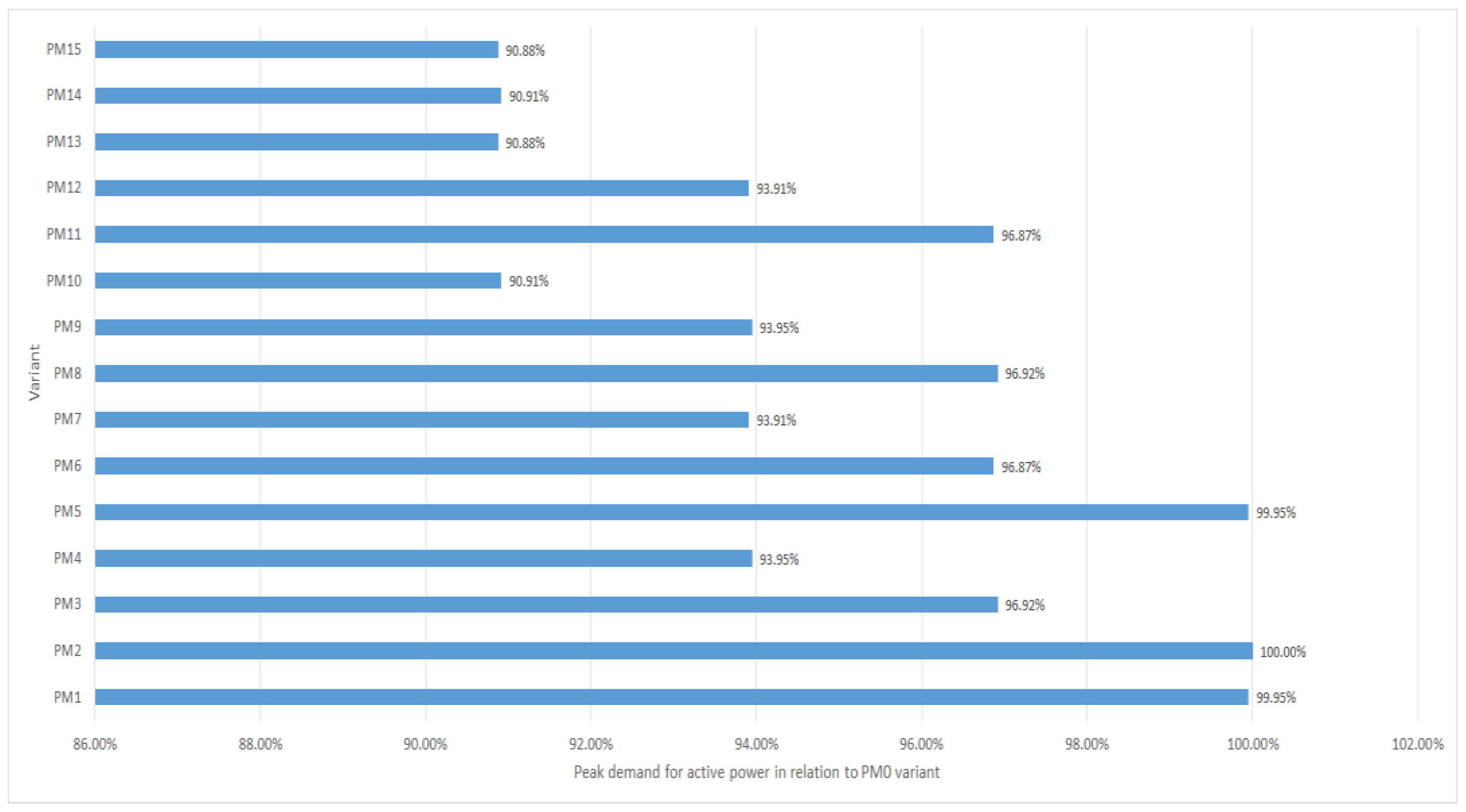
Number of Variants Composed of Several Basic Preventive MeasuresNumber of Basic Variants
PM1PM2PM3PM4
PM5YesYesNoNo
PM6YesNoYesNo
PM7YesNoNoYes
PM8NoYesYesNo
PM9NoYesNoYes
PM10NoNoYesYes
PM11YesYesYesNo
PM12YesYesNoYes
PM13YesNoYesYes
PM14NoYesYesYes
PM15YesYesYesYes
Table 2. Relative metrics of energy efficiency.
ParameterValue
MS_observ_Ep sum [kWh]557,011.669
MS_observ_Ep_new sum [kWh]556,037.796
MS_obser_Ep saved energy [%]0.175
MS_observ_Eq sum [kVarh]119,219.739
MS_observ_Eq_new sum [kVarh]119,231.689
MS_obser_Eq saved energy [%]−0.010
Disclaimer/Publisher’s Note: The statements, opinions and data contained in all publications are solely those of the individual author(s) and contributor(s) and not of MDPI and/or the editor(s). MDPI and/or the editor(s) disclaim responsibility for any injury to people or property resulting from any ideas, methods, instructions or products referred to in the content.

