Synergistic Framework for Fuel Cell Mass Transport Optimization: Coupling Reduced-Order Models with Machine Learning Surrogates

Abstract

Facing the complex coupled process of thermal mass transfer and electrochemical reaction inside fuel cells, the development of a one-dimensional model is an efficient solution to study the influence of mass transfer property parameters on the transfer and reaction process, which can effectively balance the computational efficiency and accuracy. Firstly, a one-dimensional two-phase non-isothermal parametric model is established to capture the performance and state of fuel cell quickly. Then, a sensitivity analysis is performed on various mass transfer parameters of the membrane electrode assembly. Subsequently, a neural network surrogate model and genetic algorithm are combined to optimize the mass transfer property parameters globally. The impact of these parameters on the thermal and mass transfer within the fuel cell is analyzed. The results show that the maximum error between the calculation results of the developed numerical model and the experimental results is 3.87%, and the maximum error between the predicted values of the trained surrogate model and the true values is 0.15%. The mass transfer characteristics of the gas diffusion layer have the most significant impact on the performance of the fuel cell. After optimizing the mass transfer characteristic parameters, the net power density of the fuel cell increased by 5.51%. The combination of the one-dimensional model, the surrogate model, and the genetic algorithm can effectively improve the optimization efficiency.

1. Introduction

Under the dual-carbon policy background, hydrogen fuel cells (FCs) have garnered significant research attention. Proton exchange membrane fuel cells (PEMFCs) demonstrate particular promise for commercial deployment in heavy-duty commercial vehicles owing to their advantageous characteristics including low operating temperature, high power density (P_d), rapid load response capability, low noise emission, and zero-pollution operation [1]. However, the operational requirements of heavy-duty commercial vehicles characterized by long-distance operation, high-intensity usage, and substantial load demands impose stringent performance criteria on FC systems in terms of durability, stability, and operational efficiency. The establishment of efficient and stable heat and mass transfer processes within these systems remains a critical technical challenge. Current research focuses on enhancing heat and mass transfer capabilities through optimization of two primary components: the bipolar plate flow field and the membrane electrode assembly (MEA). Reactant gases delivered through the flow field must subsequently permeate the gas diffusion layer (GDL) of the MEA before reaching the catalyst layer (CL) for electrochemical reactions. Consequently, both GDL and CL serve as crucial functional components governing the coupled heat and mass transfer processes within PEMFC systems.

Regarding the mass transfer properties of GDLs, Lee et al. [2] used the three-dimensional (3D) lattice Boltzmann method (LBM) to study the influence of liquid water content on the thermal conductivity of GDLs. Froning et al. [3] employed a trained convolutional neural network to investigate the impact of random arrangement of GDL fibers, four types of binder distributions, and compression on permeability. Xiao et al. [4] reconstructed the real structure of GDLs through fiber tracking technology and performed pore-scale simulation to calculate the changes in stress–strain, gas diffusivity, and electrical and thermal conductivity under different compression ratios. Ye et al. [5] analyzed the deflection of GDL fibers in the thickness direction and applied 3D LBM to study the contribution of different structures and property parameters to the liquid water transport process.

Regarding mass transport characteristics in CLs, He et al. [6] conducted systematic investigations using 3D LBM simulations to identify critical structural parameters governing oxygen, water vapor, and proton transport within reconstructed CL microstructures. Park et al. [7] employed LBM to analyze reactive gas transport properties under pre- and post-compression conditions, quantitatively assessing interfacial interactions between phase distributions and mass transfer processes. Chen et al. [8] implemented LBM to resolve oxygen diffusion mechanisms across CL pores and ionomer networks, with emphasis on transport dynamics at pore–ionomer interfaces. Liu et al. [9] developed a 3D computational fluid dynamics model to evaluate how anisotropic mass transport properties in dual dimensions influence the transient performance of FCs.

The 3D numerical models enable precise characterization of energy and mass spatial distributions within the MEA, thereby facilitating targeted optimization of internal structures and material properties. However, the computational demands of such high-fidelity simulations require substantial hardware resources and temporal investments, typically limiting their application to microscale investigations while remaining inadequate for analyzing full-component configurations or coupled transport phenomena across multiple components. In contrast, one-dimensional (1D) models [10] demonstrate exceptional computational efficiency in capturing fundamental FC behaviors, making them particularly valuable for preliminary parameter optimization, real-time performance monitoring, and dynamic control applications, all critical considerations for engineering implementations. Numerous studies have successfully employed 1D modeling frameworks to advance FC development through operational parameter refinement [11], gas channel (GC) flow pattern prediction [12], and MEA structural optimization [13], establishing their practical significance in component design guidance. Nevertheless, current modeling efforts predominantly focus on elucidating how MEA structural modifications influence individual mass transport characteristics, while systematic investigations into the coupled heat–mass transfer mechanisms governing overall FC performance remain notably scarce.

Motivated by these research considerations, this study developed a steady-state 1D parameterized model incorporating two-phase non-isothermal conditions to systematically investigate critical mass transport properties governing FC performance. The proposed framework enabled comprehensive analysis of spatial distributions for key physical quantities and their collective impacts on performance output under varying transport properties. To advance beyond conventional parametric studies, we further integrated an artificial neural network (ANN)-based surrogate model with genetic algorithm optimization protocols. This hybrid computational strategy effectively identified dominant mass transfer parameters and determined their optimal values through multi-objective performance maximization, establishing a novel methodology for rational MEA design optimization.

2. Materials and Methods

The 1D numerical model of the PEMFC developed in this study specifically focused on the MEA component, with GC and bipolar plates simplified as boundary conditions for the MEA. The MEA was conceptualized as five adjacent subdomains: a central proton exchange membrane (PEM) flanked by paired CLs and GDLs on both anode and cathode sides, as schematically illustrated in Figure 1. This formulation accounts for the transport and mutual coupling of eight critical physical variables across these subdomains.

2.1. Model Assumptions

The following assumptions were applied in model development: (1) ideal gas law and Fick’s laws govern gaseous species behavior; (2) convective transport of gases within the MEA was neglected; (3) the PEM completely blocked gas permeation, electronic conduction, and liquid water penetration; (4) the system operated under steady-state conditions; (5) generated liquid water was efficiently removed by gas stream purging; and (6) material properties remained uniformly distributed throughout all MEA components.

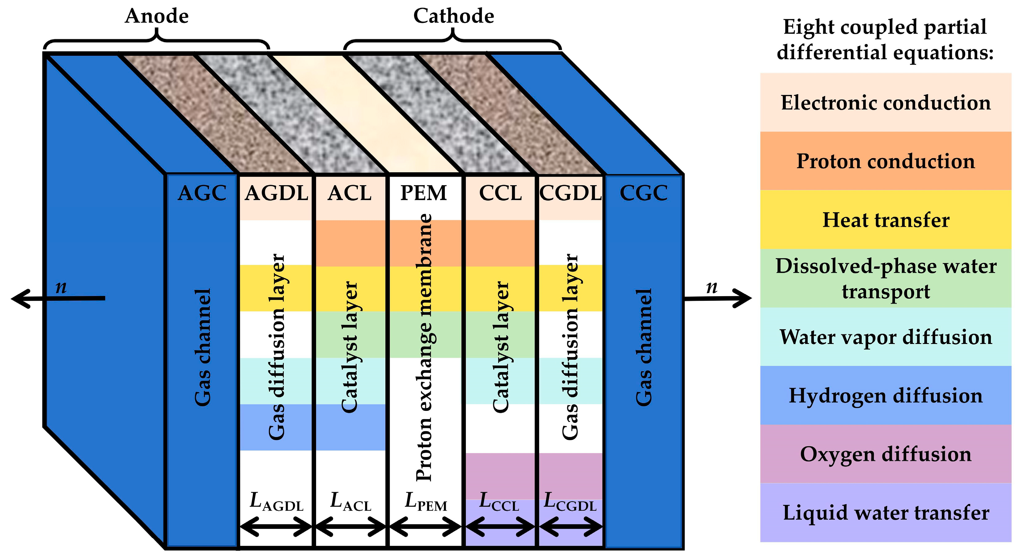
2.2. Governing Equations

The transport phenomena of water, heat, charge, and gaseous species within the FC are governed by a system of coupled partial differential equations (PDEs), which form the foundation for numerical simulations of FC performance. As summarized in

Table 1. Governing equations.

Name	Variable	Flux	Continuity Equation
Electronic conduction	${\mathit{\varphi }}_{\mathrm{e}}$	$j_{\mathrm{e}}=-{\mathit{\sigma }}_{\mathrm{e}}\nabla {\mathit{\varphi }}_{\mathrm{e}}$	$\nabla \cdot j_{\mathrm{e}}=S_{\mathrm{e}}$
Proton conduction	${\mathit{\varphi }}_{\mathrm{m}}$	$j_{\mathrm{m}}=-{\mathit{\sigma }}_{\mathrm{m}}\nabla {\mathit{\varphi }}_{\mathrm{m}}$	$\nabla \cdot j_{\mathrm{m}}=S_{\mathrm{m}}$
Heat transfer	T	$j_T=-k\nabla T$	$\nabla \cdot j_T=S_T$
Water transport in ionomers	λ	$j_{\mathit{\lambda }}=-\left(D_{\mathit{\lambda }}/V_{\mathrm{m}}\right)\nabla \mathit{\lambda }+\left(n_{\mathrm{d}}/F\right)j_{\mathrm{m}}$	$\nabla \cdot j_{\mathit{\lambda }}=S_{\mathit{\lambda }}$
Water vapor diffusion	$x_{{\mathrm{H}}_2\mathrm{O}}$	$j_{{\mathrm{H}}_2\mathrm{O}}=-C{D}_{{\mathrm{H}}_2\mathrm{O}}\nabla x_{{\mathrm{H}}_2\mathrm{O}}$	$\nabla \cdot j_{{\mathrm{H}}_2\mathrm{O}}=S_{{\mathrm{H}}_2\mathrm{O}}$
Hydrogen diffusion	$x_{{\mathrm{H}}_2}$	$j_{{\mathrm{H}}_2}=-C{D}_{{\mathrm{H}}_2}\nabla x_{{\mathrm{H}}_2}$	$\nabla \cdot j_{{\mathrm{H}}_2}=S_{{\mathrm{H}}_2}$
Oxygen diffusion	$x_{{\mathrm{O}}_2}$	$j_{{\mathrm{O}}_2}=-C{D}_{{\mathrm{O}}_2}\nabla x_{{\mathrm{O}}_2}$	$\nabla \cdot j_{{\mathrm{O}}_2}=S_{{\mathrm{O}}_2}$
Liquid water transfer	s	$j_s=-\left(\mathit{\kappa }/\mathit{\mu }{V}_{\mathrm{w}}\right)\left(\partial p_{\mathrm{c}}/\partial s\right)\nabla s$	$\nabla \cdot j_s=S_s$

, eight governing equations corresponding to key variables were formulated. Each independent variable is represented by a different color in Figure 1, and the corresponding areas where each variable is transmitted are marked in the MEA section. Taking heat transfer as an example, by observing the range covered by the yellow area in the figure, it was found that the heat transport runs through all parts of the MEA. The continuity equation for each variable establishes the relationship between its flux and the corresponding source term derived from physicochemical processes. All phase-change kinetics and electrochemical reaction rates were explicitly incorporated as source terms within these coupled PDEs.

2.3. Electrochemical Model

The reversible potential ($\Delta {\mathit{\varphi }}_0$) of the FC is determined by the Nernst equation [14]:

$$\Delta {\mathit{\varphi }}_0=-{\displaystyle \frac{\Delta H-T\Delta S}{2F}}+{\displaystyle \frac{RT}{2F}}\mathrm{l}\mathrm{n}\left[\left({\displaystyle \frac{p_{{\mathrm{H}}_2}}{P_{\mathrm{r}\mathrm{e}\mathrm{f}}}}\right){\left({\displaystyle \frac{p_{{\mathrm{O}}_2}}{P_{\mathrm{r}\mathrm{e}\mathrm{f}}}}\right)}^{1/2}\right]$$

(1)

where F is the Faraday constant, R is the universal gas constant, P_ref is the reference pressure (Pa), T is the operating temperature (K), and $p_{{\mathrm{H}}_2}$ and $p_{{\mathrm{O}}_2}$ represent the partial pressures of hydrogen and oxygen, respectively, expressed as:

$$p_{{\mathrm{H}}_2}=x_{{\mathrm{H}}_2}{P}_{\mathrm{a}}, p_{{\mathrm{O}}_2}=x_{{\mathrm{O}}_2}{P}_{\mathrm{c}}$$

(2)

where $x_{{\mathrm{H}}_2,{\mathrm{O}}_2}$ denote the mole fractions of hydrogen and oxygen in the anode gas channel (AGC) and cathode gas channel (CGC), respectively, and P_a and P_c are the absolute pressures in the AGC and CGC.

Suppose that the electrochemical reactions within the FC can be divided into the hydrogen oxidation reaction (HOR) in the anode catalyst layer (ACL) and the oxygen reduction reaction (ORR) in the cathode catalyst layer (CCL). The reaction rate (i) in a homogeneous catalyst layer can be derived from the Butler–Volmer equation as [15]:

$$i=i_{0,\mathrm{a}/\mathrm{c}}{A}_{\mathrm{a}/\mathrm{c}}\left[\mathrm{e}\mathrm{x}\mathrm{p}\left({\displaystyle \frac{2\beta F\eta }{RT}}\right)-\mathrm{e}\mathrm{x}\mathrm{p}\left({\displaystyle \frac{2\left(\beta -1\right)F\eta }{RT}}\right)\right]$$

(3)

where A_a/c represent the electrochemical active area of A/CCL (m⁻¹), and β is the transfer coefficient.

For the two half-reactions of the anode and cathode, the exchange current density i_0,a/c (A·m⁻²) is expressed by the following equation [16,17]:

$$i_{0,\mathrm{a}/\mathrm{c}}=\left\{\begin{array}{ll}2.7\times {10}^3\times \mathrm{e}\mathrm{x}\mathrm{p}\left[{\displaystyle \frac{1.6\times {10}^3}{R}}\left({\displaystyle \frac{1}{T_{\mathrm{r}\mathrm{e}\mathrm{f}}}}-{\displaystyle \frac{1}{T}}\right)\right],\hfill & \mathrm{H}\mathrm{O}\mathrm{R}\hfill \\ 2.45\times {10}^{-4}{\left({\displaystyle \frac{p_{{\mathrm{O}}_2}}{P_{\mathrm{r}\mathrm{e}\mathrm{f}}}}\right)}^{0.54}\times \mathrm{e}\mathrm{x}\mathrm{p}\left[{\displaystyle \frac{6.7\times {10}^4}{R}}\left({\displaystyle \frac{1}{T_{\mathrm{r}\mathrm{e}\mathrm{f}}}}-{\displaystyle \frac{1}{T}}\right)\right],\hfill & \mathrm{O}\mathrm{R}\mathrm{R}\hfill \end{array}\right.$$

(4)

The activation overpotential (η) is expressed by the following equation:

$$\eta =\left\{\begin{array}{cc}\Delta \mathit{\varphi }-\Delta {\mathit{\varphi }}_0,& \mathrm{A}\mathrm{C}\mathrm{L}\\ \Delta {\mathit{\varphi }}_0-\Delta \mathit{\varphi },& \mathrm{C}\mathrm{C}\mathrm{L}\end{array}\right.$$

(5)

where Δϕ is the potential difference between the electron and proton phases ($\Delta \mathit{\varphi }={\mathit{\varphi }}_{\mathrm{e}}-{\mathit{\varphi }}_{\mathrm{m}}$), and the reversible potential difference (Δϕ₀) is [18]:

$$\Delta {\mathit{\varphi }}_0=\left\{\begin{array}{ll}-{\displaystyle \frac{T\Delta S_{\mathrm{H}\mathrm{O}\mathrm{R}}}{2F}}-{\displaystyle \frac{RT}{2F}}\mathrm{l}\mathrm{n}\left({\displaystyle \frac{p_{{\mathrm{H}}_2}}{P_{\mathrm{r}\mathrm{e}\mathrm{f}}}}\right),\hfill & \mathrm{A}\mathrm{C}\mathrm{L}\hfill \\ -{\displaystyle \frac{\Delta H-T\Delta S_{\mathrm{O}\mathrm{R}\mathrm{R}}}{2F}}+{\displaystyle \frac{RT}{4F}}\mathrm{l}\mathrm{n}\left({\displaystyle \frac{p_{{\mathrm{o}}_2}}{P_{\mathrm{r}\mathrm{e}\mathrm{f}}}}\right),\hfill & \mathrm{C}\mathrm{C}\mathrm{L}\hfill \end{array}\right.$$

(6)

where ∆S_HOR and ∆S_ORR are, respectively, the entropy values of the anode and cathode half-reactions.

2.4. Source Terms and Phase Changes

The definitions of the source terms corresponding to the eight control equations in each region are shown in

Table 2. Source terms.

Source Terms	AGDL	ACL	PEM	CCL	CGDL
Se	0	−i	-	i	0
Sm	-	i	0	−i	-
ST	$S_{\mathrm{T},\mathrm{e}}$	$S_{\mathrm{T},\mathrm{e}}+S_{\mathrm{T},\mathrm{m}}+S_{\mathrm{T},\mathrm{r}}+S_{\mathrm{T},\mathrm{ad}}$	$S_{\mathrm{T},\mathrm{p}}$	$S_{\mathrm{T},\mathrm{e}}+S_{\mathrm{T},\mathrm{m}}+S_{\mathrm{T},\mathrm{r}}+S_{\mathrm{T},\mathrm{ad}}+S_{\mathrm{T},\mathrm{ec}}$	$S_{\mathrm{T},\mathrm{e}}+S_{\mathrm{T},\mathrm{e}\mathrm{c}}$
Sλ	-	Sad	0	i/2F + Sad	-
$S_{{\mathrm{H}}_2\mathrm{O}}$	0	−Sad	-	−Sad − Sec	−Sec
$S_{{\mathrm{H}}_2}$	0	−i/2F	-	-	-
$S_{{\mathrm{O}}_2}$	-	-	-	−i/4F	0
Ss	-	-	-	Sec	Sec

. The specific expressions corresponding to each source term are detailed below.

The membrane water content (λ) and the adsorption source term (S_ad) appearing in the continuity equation are set as [19]:

$$S_{\mathrm{a}\mathrm{d}}=\left\{\begin{array}{cc}{k}_{\mathrm{a}}\left({\mathit{\lambda }}_{\mathrm{e}\mathrm{q}}-\mathit{\lambda }\right)/L_{\mathrm{C}\mathrm{L}}{V}_{\mathrm{m}},& \mathit{\lambda }<{\mathit{\lambda }}_{\mathrm{e}\mathrm{q}}(\mathrm{a}\mathrm{d}\mathrm{s}\mathrm{o}\mathrm{r}\mathrm{p}\mathrm{t}\mathrm{i}\mathrm{o}\mathrm{n})\\ k_{\mathrm{d}}\left({\mathit{\lambda }}_{\mathrm{e}\mathrm{q}}-\mathit{\lambda }\right)/L_{\mathrm{C}\mathrm{L}}{V}_{\mathrm{m}},& \mathit{\lambda }>{\mathit{\lambda }}_{\mathrm{e}\mathrm{q}}(\mathrm{d}\mathrm{e}\mathrm{s}\mathrm{o}\mathrm{r}\mathrm{p}\mathrm{t}\mathrm{i}\mathrm{o}\mathrm{n})\end{array}\right.$$

(7)

where L_CL represents the thickness of CL (m), V_m is the molar charge volume of the ionomer (m³·mol⁻¹), λ_eq indicates the equilibrium water content, and k_a,d is the mass transfer coefficient of water vapor in the membrane.

In macroscopic homogeneous MEA modeling, it is assumed that mass transfer is driven by the difference between the vapor partial pressure and the saturation pressure (P_sat), and the corresponding source/sink term can be expressed as:

$$S_{\mathrm{e}\mathrm{c}}=\left\{\begin{array}{ll}{\mathit{\gamma }}_{\mathrm{e}}C\left(x_{{\mathrm{H}}_2\mathrm{O}}-x_{\mathrm{s}\mathrm{a}\mathrm{t}}\right),\hfill & x_{{\mathrm{H}}_2\mathrm{O}}<x_{\mathrm{s}\mathrm{a}\mathrm{t}}\left(\mathrm{E}\mathrm{v}\mathrm{a}\mathrm{p}\mathrm{o}\mathrm{r}\mathrm{a}\mathrm{t}\mathrm{i}\mathrm{o}\mathrm{n}\right)\hfill \\ {\mathit{\gamma }}_{\mathrm{c}}C\left(x_{{\mathrm{H}}_2\mathrm{O}}-x_{\mathrm{s}\mathrm{a}\mathrm{t}}\right),\hfill & x_{{\mathrm{H}}_2\mathrm{O}}>x_{\mathrm{s}\mathrm{a}\mathrm{t}}\left(\mathrm{C}\mathrm{o}\mathrm{n}\mathrm{d}\mathrm{e}\mathrm{n}\mathrm{s}\mathrm{a}\mathrm{t}\mathrm{i}\mathrm{o}\mathrm{n}\right)\hfill \end{array}\right.$$

(8)

where x_sat = P_sat/P, and γ_e and γ_c are the evaporation and condensation rates, respectively.

The expressions for the latent heat released or absorbed in the above two-phase transition processes are:

$$\begin{array}{l}{S}_{\mathrm{T},\mathrm{a}\mathrm{d}}=H_{\mathrm{a}\mathrm{d}}{S}_{\mathrm{a}\mathrm{d}}\\ S_{\mathrm{T},\mathrm{e}\mathrm{c}}=H_{\mathrm{e}\mathrm{c}}{S}_{\mathrm{e}\mathrm{c}}\end{array}$$

(9)

where H_ad and H_ec are the molar enthalpies of desorption and evaporation (J·mol⁻¹), respectively.

The two ohmic heat sources caused by electron and ion conduction are:

$$\begin{array}{l}{S}_{\mathrm{T},\mathrm{e}}={\mathit{\sigma }}_{\mathrm{e}}{\left(\nabla {\mathit{\varphi }}_{\mathrm{e}}\right)}^2=-j_{\mathrm{e}}\cdot \nabla {\mathit{\varphi }}_{\mathrm{e}}\hfill \\ S_{\mathrm{T},\mathrm{m}}={\mathit{\sigma }}_{\mathrm{m}}{\left(\nabla {\mathit{\varphi }}_{\mathrm{m}}\right)}^2=-j_{\mathrm{m}}\cdot \nabla {\mathit{\varphi }}_{\mathrm{m}}\hfill \end{array}$$

(10)

The heat dissipated by the electrochemical reaction is [20]:

$$S_{\mathrm{T},\mathrm{r}}=i\eta -{\displaystyle \frac{i}{2F}}\times \left\{\begin{array}{cc}T\Delta S_{\mathrm{H}\mathrm{O}\mathrm{R}}& \mathrm{A}\mathrm{C}\mathrm{L}\\ T\Delta S_{\mathrm{O}\mathrm{R}\mathrm{R}}& \mathrm{C}\mathrm{C}\mathrm{L}\end{array}\right.$$

(11)

The property expressions and parameter values involved in the above formulas are shown in

Table 3. Expressions of each property [21].

Property/Unit	Expression	Property/Unit	Expression
Saturated pressure of water vapor/Pa	$\begin{array}{ll}\mathrm{l}\mathrm{o}{\mathrm{g}}_{10}{P}_{\mathrm{s}\mathrm{a}\mathrm{t}}=& -2.1794+0.02953\left(T-273.17\right)\\ & -9.1837\times 10^{-5}{\left(T-273.17\right)}^2\\ & +1.4454\times 10^{-7}{\left(T-273.17\right)}^3\end{array}$	Dynamic viscosity of liquid water/mPa·s	$\mathrm{l}\mathrm{n}\mathit{\mu }=-3.63148+{\displaystyle \frac{542.05}{T-144.15}}$
Water vapor mass transfer coefficient in the membrane/m·s−1	$k_{\mathrm{a},\mathrm{d}}=a_{\mathrm{a},\mathrm{d}}f\mathrm{e}\mathrm{x}\mathrm{p}\left[{\displaystyle \frac{2\times {10}^4}{R}}\left({\displaystyle \frac{1}{T_{\mathrm{r}\mathrm{e}\mathrm{f}}}}-{\displaystyle \frac{1}{T}}\right)\right]$	The volume fraction of water in the ionomer/-	$f={\displaystyle \frac{\mathit{\lambda }{V}_{\mathrm{w}}}{\mathit{\lambda }{V}_{\mathrm{w}}+V_{\mathrm{m}}}}$
Capillary pressure/Pa	$p_{\mathrm{c}}=\mathit{\sigma }\left|\mathrm{c}\mathrm{o}\mathrm{s}{\mathit{\theta }}_{\mathrm{c}}\right|\sqrt{{\displaystyle \frac{{\mathit{\epsilon }}_{\mathrm{p}}}{{\mathit{\kappa }}_{\mathrm{a}\mathrm{b}\mathrm{s}}}}}\left(\begin{array}{l}1.417s-2.12s^2\\ +1.263s^3\end{array}\right)$	Electrophoretic resistance coefficient/-	$n_{\mathrm{d}}={\displaystyle \frac{2.5\mathit{\lambda }}{22}}$
Equilibrium water content of the ionomer/-	$\begin{array}{ll}{\mathit{\lambda }}_{\mathrm{e}\mathrm{q}}& =0.3+6a\left[1-\mathrm{t}\mathrm{a}\mathrm{n}\mathrm{h}\left(a-0.5\right)\right]+7.6s\\ & + 3.9192a^{0.5}\left[1+\mathrm{t}\mathrm{a}\mathrm{n}\mathrm{h}\left({\displaystyle \frac{a-0.89}{0.23}}\right)\right]\end{array}$	Water activity/-	$a=P_{{\mathrm{H}}_2\mathrm{O}}/P_{\mathrm{s}\mathrm{a}\mathrm{t}}$
Concentration of interstitial gas/mol·m−3	C = P/RT	Hydraulic permeability/m²	$\mathit{\kappa }=\left(10^{-6}+s_{\mathrm{r}\mathrm{e}\mathrm{d}}^3\right){\mathit{\kappa }}_{\mathrm{a}\mathrm{b}\mathrm{s}}$
Water diffusion rate in the ionomer/m²·s−1	$D_{\mathit{\lambda }}={\displaystyle \frac{{\rho }_i}{EW}}\times \left\{\begin{array}{l}\begin{array}{l}3.1\times 10^{-3}\mathit{\lambda }\left[\mathrm{e}\mathrm{x}\mathrm{p}\left(0.28\mathit{\lambda }\right)-1\right]\\ \mathrm{e}\mathrm{x}\mathrm{p}\left(-2346/\mathrm{T}\right),0<\mathit{\lambda }\le 3\end{array}\hfill \\ \begin{array}{l}4.17\times 10^{-4}\mathit{\lambda }\left[1+161\mathrm{e}\mathrm{x}\mathrm{p}\left(-\mathit{\lambda }\right)\right]\\ \mathrm{e}\mathrm{x}\mathrm{p}\left(-2346/\mathrm{T}\right),\mathit{\lambda }>3\end{array}\hfill \end{array}\right.$	Fickean gas diffusion rate/m²·s−1	$\begin{array}{l}{D}_{\mathrm{i}}={\displaystyle \frac{{\mathit{\epsilon }}_{\mathrm{p}}}{{\mathit{\tau }}^{\mathrm{2}}}}(1-s{)}^3{D}_{\mathrm{i},\mathrm{r}\mathrm{e}\mathrm{f}}{\left({\displaystyle \frac{T}{T_{\mathrm{r}\mathrm{e}\mathrm{f}}}}\right)}^{1.5}{\displaystyle \frac{P_{\mathrm{r}\mathrm{e}\mathrm{f}}}{P}}\\ i={\mathrm{H}}_2,{\mathrm{O}}_2,{\mathrm{H}}_2\mathrm{O}\end{array}$
Evaporation and condensation rates/s−1	${\mathit{\gamma }}_{\mathrm{e},\mathrm{c}}=k_{\mathrm{e},\mathrm{c}}{a}_{\mathrm{l}\mathrm{g}}\times \left\{\begin{array}{ll}{s}_{\mathrm{r}\mathrm{e}\mathrm{d}},\hfill & \mathrm{E}\mathrm{v}\mathrm{a}\mathrm{p}\mathrm{o}\mathrm{t}\mathrm{r}\mathrm{a}\mathrm{t}\mathrm{i}\mathrm{o}\mathrm{n}\hfill \\ 1-s_{\mathrm{r}\mathrm{e}\mathrm{d}},\hfill & \mathrm{C}\mathrm{o}\mathrm{n}\mathrm{d}\mathrm{e}\mathrm{n}\mathrm{s}\mathrm{a}\mathrm{t}\mathrm{i}\mathrm{o}\mathrm{n}\hfill \end{array}\right.$	Hertz–Knudsen mass transfer coefficient/m·s−1	$\begin{array}{ll}{k}_{\mathrm{e},\mathrm{c}}=& \sqrt{{\displaystyle \frac{RT}{2\mathit{\pi }{M}_{\mathrm{W}}}}}\\ & \times \left\{\begin{array}{ll}5\times 10^{-4},\hfill & \mathrm{E}\mathrm{v}\mathrm{a}\mathrm{p}\mathrm{o}\mathrm{r}\mathrm{a}\mathrm{t}\mathrm{i}\mathrm{o}\mathrm{n}\hfill \\ 6\times 10^{-3},\hfill & \mathrm{C}\mathrm{o}\mathrm{n}\mathrm{d}\mathrm{e}\mathrm{n}\mathrm{s}\mathrm{a}\mathrm{t}\mathrm{i}\mathrm{o}\mathrm{n}\hfill \end{array}\right.\end{array}$
Ion conductivity of the membrane/S·m−1	$\begin{array}{ll}{\mathit{\sigma }}_{\mathrm{m}}=& {\mathit{\epsilon }}_{\mathrm{i}}\left(0.514\mathit{\lambda }-0.326\right)\\ & \times \mathrm{e}\mathrm{x}\mathrm{p}\left[1268\left({\displaystyle \frac{1}{303.15}}-{\displaystyle \frac{1}{T}}\right)\right]\end{array}$	Reduced saturation/-	$s_{\mathrm{r}\mathrm{e}\mathrm{d}}={\displaystyle \frac{s-0.12}{1-0.12}}$

and

Table 4. Values of each parameter in the equation [22].

Parameters/Symbols	Value/Unit	Parameters/Symbols	Value/Unit
The equivalent volume of dry film/Vm	517.766/cm3·mol−1	The molar volume of liquid water/Vw	18.405/cm3·mol−1
Latent heat of evaporation/condensation/Had,ec	42/kJ·mol−1	Transfer coefficient/β	0.5/−
Adsorption mass transfer coefficient/aa	3.53 × 10−5/m·s−1	Desorption mass transfer coefficient/ad	1.42 × 10−4/m·s−1
Entropy value of the anode half-reaction/∆SHOR	0.104/J (mol K)−1	Entropy value of the cathode half-reaction /∆SORR	−163.3/J (mol K)−1
The electrochemically active area of anode CL/Aa	1 × 107/m−1	The electrochemically active area of the cathode CL/Ac	3 × 107/m−1
Effective liquid-gas interface area density ratio factor/alg	2 × 106/m−1	The molar mass of water/Mw	18/g·mol−1

.

3. Coupled Solution and Verification of the Model

Based on the mathematical model given above, MATLAB R2024a code was written. Subsequently, boundary and initial conditions were imposed, and then the application and validity of the model were verified. The specific process is as follows.

3.1. Boundary and Initial Conditions

(1)

Boundary Conditions

To fully describe the model, it is necessary to specify the boundary conditions as shown in

Table 5. Boundary conditions [18].

Variable	AGC/AGDL	AGDL/ACL	ACL/PEM	PEM/CCL	CCL/CGDL	CGDL/CGC
ϕe	${\mathit{\varphi }}_{\mathrm{e}}=0$	Continuity	$n\cdot j_{\mathrm{e}}=0$	$n\cdot j_{\mathrm{e}}=0$	Continuity	${\mathit{\varphi }}_{\mathrm{e}}=V_{\mathrm{c}\mathrm{e}\mathrm{l}\mathrm{l}}$
ϕm	-	$n\cdot j_{\mathrm{m}}=0$	Continuity	Continuity	$n\cdot j_{\mathrm{m}}=0$	-
T	T = Ta	Continuity	Continuity	Continuity	Continuity	T = Tc
λ	-	$n\cdot j_{\mathit{\lambda }}=0$	Continuity	Continuity	$n\cdot j_{\mathit{\lambda }}=0$	-
$x_{{\mathrm{H}}_2\mathrm{O}}$	$x_{{\mathrm{H}}_2\mathrm{O}}=x_{{\mathrm{H}}_2\mathrm{O}}^{\mathrm{a}}$	Continuity	$n\cdot j_{{\mathrm{H}}_2\mathrm{O}}=0$	$n\cdot j_{{\mathrm{H}}_2\mathrm{O}}=0$	Continuity	$x_{{\mathrm{H}}_2\mathrm{O}}=x_{{\mathrm{H}}_2\mathrm{O}}^{\mathrm{c}}$
$x_{{\mathrm{H}}_2}$	$x_{{\mathrm{H}}_2}=x_{{\mathrm{H}}_2}^{\mathrm{a}}$	Continuity	$n\cdot j_{{\mathrm{H}}_2}=0$	-	-	-
$x_{{\mathrm{O}}_2}$	-	-	-	$n\cdot j_{{\mathrm{O}}_2}=0$	Continuity	$x_{{\mathrm{O}}_2}=x_{{\mathrm{O}}_2}^{\mathrm{c}}$
s	-	-	-	$n\cdot j_s=0$	Continuity	$s=s_{\mathrm{c}}$

, where n represents the unit normal vector of the interface. According to model assumption (3), the fluxes of gas, electrons and liquid water vanish at the PEM boundary. The proton, dissolved water, and the ionomer combine, resulting in zero fluxes of the two on the outer surface of the CL. The boundary involved in the table also includes the CGDL. On the remaining internal subdomain interfaces, it was assumed that the potential and fluxes are continuous.

The relationships among various external operation condition parameters are as follows:

$$\begin{array}{l}{x}_{{\mathrm{H}}_2\mathrm{O}}^{\mathrm{a}}=\mathrm{R}{\mathrm{H}}_{\mathrm{a}}{P}_{\mathrm{s}\mathrm{a}\mathrm{t}}(T_{\mathrm{a}})/P_{\mathrm{a}}\\ x_{{\mathrm{H}}_2\mathrm{O}}^{\mathrm{c}}=\mathrm{R}{\mathrm{H}}_{\mathrm{c}}{P}_{\mathrm{s}\mathrm{a}\mathrm{t}}(T_{\mathrm{c}})/P_{\mathrm{c}}\\ x_{{\mathrm{H}}_2}^{\mathrm{a}}={\mathit{\alpha }}_{{\mathrm{H}}_2}(1-x_{{\mathrm{H}}_2\mathrm{O}}^{\mathrm{a}})\\ x_{{\mathrm{O}}_2}^c={\mathit{\alpha }}_{{\mathrm{O}}_2}(1-x_{{\mathrm{H}}_2\mathrm{O}}^{\mathrm{c}})\end{array}$$

(12)

where RH represents the relative humidity, and ${\mathit{\alpha }}_{{\mathrm{H}}_2}$(${\mathit{\alpha }}_{{\mathrm{O}}_2}$) represents the molar fraction of hydrogen (oxygen) in the supply gas during drying.

(2)

Initial Conditions

To ensure good convergence of the iterative solver for solving non-linear problems, in this study, a full zero flux was taken as the initial estimate, and the FC voltage (V_cell) was iterated from high to low to generate the polarization curve. For the potential, the following initial conditions are usually sufficient for convergence: ϕ_e ≡ (0|V_cell), ϕ_m ≡ 0, T ≡ (T_a + T_c)/2, λ ≡ λ_{eq|RH = 1}, $x_{{\mathrm{H}}_2\mathrm{O}}\equiv (x_{{\mathrm{H}}_2\mathrm{O}}^{\mathrm{a}}|x_{{\mathrm{H}}_2\mathrm{O}}^{\mathrm{c}})$, $x_{{\mathrm{H}}_2}\equiv x_{{\mathrm{H}}_2}^{\mathrm{a}}$, $x_{{\mathrm{O}}_2}\equiv x_{{\mathrm{O}}_2}^{\mathrm{c}}$, s ≡ s_c, where the symbols (a, c) represent A/CGDL and A/CCL, respectively. The properties of all materials in the model are shown in

Table 6. Material and mass transfer parameters in the through-plane direction [23].

Symbol	Explanation	Unit	AGDL and CGDL	ACL and CCL	PEM
L	Thickness	μm	160	10	25
εi	Volume fraction of ionomer	-	-	0.3	1
εp	Porosity	-	0.76	0.4	-
k	Thermal conductivity	W·(m·K)−1	1.6	0.27	0.3
τ	Pore tortuosity	-	1.6	1.6	-
κabs	Absolute permeability	m2	6.15 × 10−12	1 × 10−13	-
σe	Electrical conductivity	S·m−1	1250	350	-
θc	Contact angle	°	120	100	-

.

3.2. Numerical Application of the Model and Validation of Its Effectiveness

(1)

Application Process of the Model

This model was implemented as an independent MATLAB function, and the coupled equations were solved using MATLAB’s boundary value problem solver for ordinary differential equations, bvp4c [21], which is a finite difference solver that implements a three-stage Lobatto IIIa implicit Runge–Kutta method with automatic mesh selection based on residuals, providing a fourth-order accurate piecewise C¹ continuous solution. On a computer with a CPU configured as AMD Ryzen9 7950X3D (Advanced Micro Devices (China) Co., Ltd., Beijing City, China), the operation time for a comprehensive scan of all V_cell values with a step size of 50 mV was just a few seconds.

(2)

Validation Process of the Model

To verify the validity of the model, the data obtained from simulation and experiment were compared. The results and the experimental equipment are shown in Figure 2. The test bench (model: JRD-SYT2K01) used in the experiment was provided by Shaoxing Junji Energy Technology Co., Ltd (Shaoxing City, Zhejiang Province, China). The flow field structure of the FC used was a parallel flow field. The specific models of the MEA are as follows: the model of the PEM is DuPont N1110 (DuPont China Group Co., Ltd., Shenzhen City, Guangdong Province, China); the model of the GDL is Freudenberg H24C × 483 (Freudenberg Performance Materials Group, Changzhou City, Jiangsu Province, China); the models of the ACL and CCL are Johnson Matthey HISPEC4000 and HISPEC9100 (Johnson Matthey (Shanghai) Chemicals Co., Ltd., Shanghai City, China), respectively. The external operating conditions of the experiment and simulation were kept consistent, with the A/CGC pressure at 1.5 atm and the relative humidity within the A/CGC at 90%. The operating temperature of the FC was 70 °C. Figure 2a shows the FC test system used in this study, which could stably capture the performance data of the FC stack with an accuracy of 100 μA and 0.1 mV. The experiment was repeated three times under the same steps and the average value was taken. Then, the performance of the stack was converted to that of a single cell through conversion. Figure 2b shows the comparison of the FC polarization performance between simulation and experiment. The maximum deviation between the simulation results and the actual performance was 3.87%, which was within the acceptable range. For comparison, the model prediction error in reference [12] is less than 10%, the maximum model prediction error in reference [24] is 4%, and in reference [25], the maximum model prediction errors in the two sets of polarization curves are 6.63% and 2.45%, respectively. The simulation results could well capture the three polarization regions and the changing trends in the actual FC. Therefore, the numerical model established in this study was valid and could be used to analyze the influence of various properties and operating parameters on the output performance of the FC.

4. Analysis and Optimization of Mass Transfer Property Parameters in the FC

To identify and optimize the key mass transfer properties of the MEA that affect FC-P_d and enhance the output performance of the FC, this study adopted an optimization process that combined a MATLAB numerical model, an ANN surrogate model, and a genetic algorithm for global optimization. The influence of each parameter was analyzed and the best parameter combination was sought.

4.1. Selection of Parameters to Be Optimized and Their Sensitivity Analysis

The water–heat–electricity–gas transfer processes and involved regions within the FC are shown in Figure 1. The heat and mass transfer properties involved are k, σ_e, and κ. As the electrochemical reaction at the cathode generates liquid water and the electroosmotic force causes the liquid water at the anode to transfer to the cathode, there is very little liquid water at the anode. Therefore, this study did not consider the mass transfer coefficient of the liquid water at the anode, i.e., κ of the AGDL and ACL. Ultimately, the heat and mass transfer parameters of the MEA considered in this study were k and σ_e of A/CGDL and A/CCL, κ of CGDL and CCL, and k of PEM, totaling 11 parameters. The value ranges for each parameter are shown in

Table 7. Proposed parameters for optimization and their value ranges.

Parameters to Be Optimized	Symbol	Range of Values	Unit
A/CGDL Thermal conductivity	kA/CGDL	[0.5, 3.5]	W·(m·K)−1
A/CGDL Electrical conductivity	${\mathit{\sigma }}_{\mathrm{e}}^{\mathrm{A}/\mathrm{C}\mathrm{G}\mathrm{D}\mathrm{L}}$	[500, 2000]	S·m−1
CGDL Permeability	κCGDL	[3, 9]	×10−12 m2
A/CCL Thermal conductivity	kA/CCL	[0.1, 0.4]	W·(m·K)−1
A/CCL Electrical conductivity	${\mathit{\sigma }}_{\mathrm{e}}^{\mathrm{A}/\mathrm{C}\mathrm{C}\mathrm{L}}$	[100, 700]	S·m−1
CCL Permeability	κCCL	[2, 20]	×10−14 m2
PEM Thermal conductivity	kPEM	[0.05, 0.5]	W·(m·K)−1

.

First, a sensitivity analysis of the heat and mass transfer properties was conducted to identify the key parameters that have a significant impact on the performance of the FC. The optimal Latin hypercube method was used to randomly sample each parameter within the optimization range, with a total of 500 sample points obtained. Each sample point is a combination of 11 parameters, and the sample points are uniformly distributed in the design space. The 500 sample points obtained through sampling were modeled and simulated, and the 1D numerical model was used for calculation to obtain the polarization performance of the FC corresponding to each sample point, which was then converted into the maximum P_d. Further, a main effect analysis was conducted to evaluate the degree of influence of each parameter on the performance of the FC.

The influence degree of each parameter on FC-P_d is shown in Figure 3. By observing the slopes of the main effect lines, it can be seen that except for k_PEM, which is negatively correlated with P_d, the other parameters are positively correlated. The parameter k_AGDL had the most significant impact on P_d, followed by k_CGDL, κ_GDL, ${\mathit{\sigma }}_{\mathrm{e}}^{\mathrm{A}\mathrm{G}\mathrm{D}\mathrm{L}}$, and ${\mathit{\sigma }}_{\mathrm{e}}^{\mathrm{C}\mathrm{G}\mathrm{D}\mathrm{L}}$. The influence of the remaining parameters on P_d was relatively small. To ensure the robustness of the model optimization, all 11 parameters were involved in the optimization design in this study.

4.2. Building a Neural Network Proxy Model

The specific process of optimizing the mass transfer properties of the FC is shown in Figure 4. In this study, a Bayesian regularization backpropagation ANN was adopted as the surrogate model, which had both good training accuracy and strong generalization ability. The maximum P_d was taken as the output response of the surrogate model, and the combination of mass transfer property parameters corresponding to the maximum P_d was used as the input variable and imported into the ANN model for training. A surrogate model was established using the 500 samples from the sensitivity analysis in the previous section, with 85% of the samples used for training and 15% as test samples. The training situation for the surrogate model is shown in Figure 5. The linear regression state of the training samples and test samples was good, and the fitted line was basically coincident with Y = T. After calculation, the correlation coefficients of the training samples, test samples, and all samples were 0.9986, 0.9933, and 0.9982, respectively. Figure 5c shows the distribution of the relative error between the predicted value and the true value. The maximum error was within 0.15%, and most of the errors were within 0.05%. These results indicate that the trained ANN surrogate model has high prediction accuracy and can be used for global optimization studies of FC within the range of various parameter values.

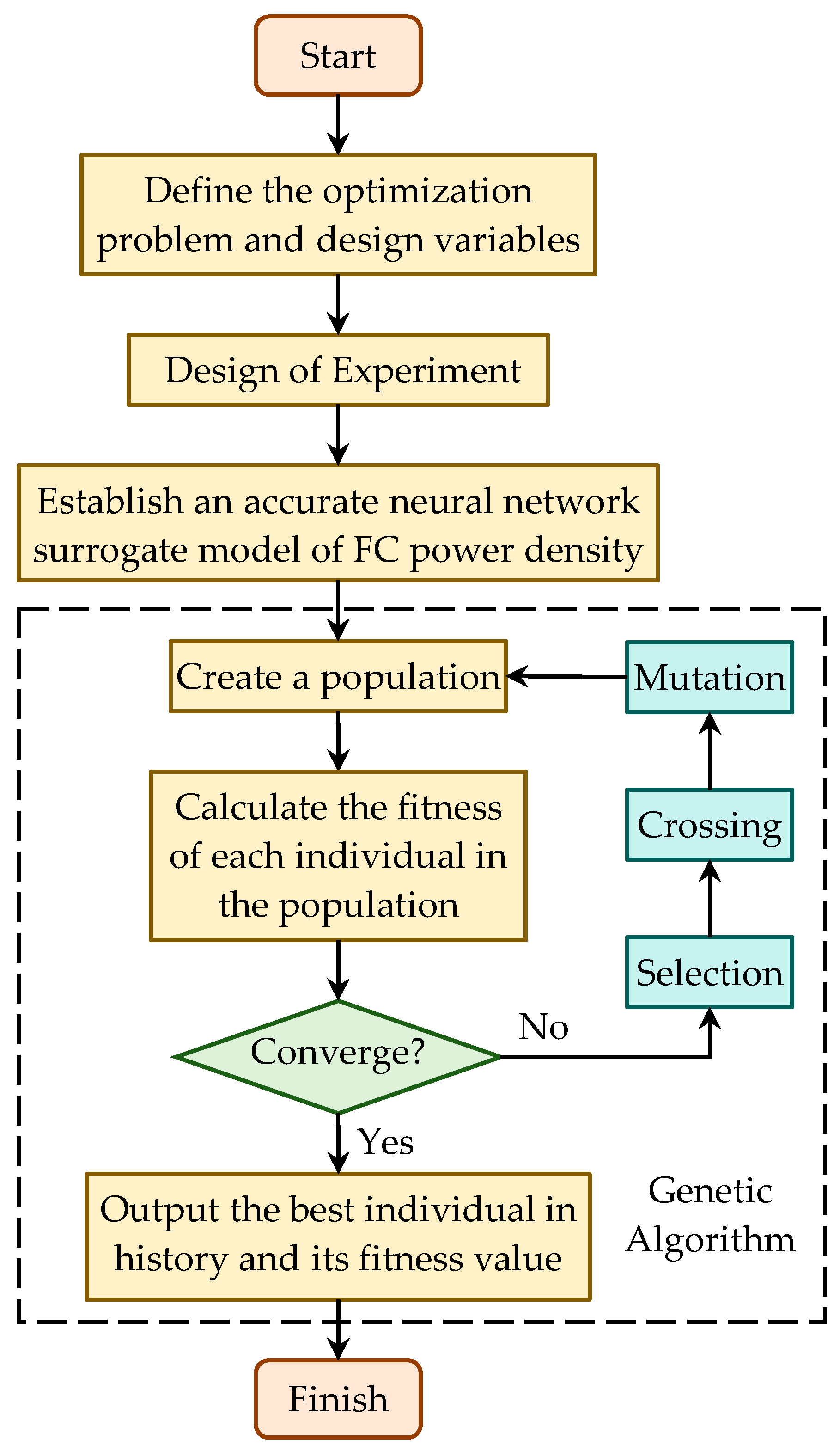
4.3. Optimization Process Based on the Genetic Algorithm

The genetic algorithm was used to optimize FC-P_d to obtain the optimal mass transfer property parameter combination with the highest P_d. The parameters of the genetic algorithm were as follows: the population size was set to 1 × 10⁴, the proportion of elite individuals was set to 0.05, and the crossover ratio was 0.8. The convergence stop condition was that the average relative change in the best fitness function value in the last 10 generations was less than 1 × 10⁻⁶. The iteration of the maximum P_d of the FC converged at the 32nd step, and the global maximum FC output P_d was obtained as 0.9191 W·cm⁻². The best heat and mass transfer parameter combination obtained, as well as the rounded parameter combination, are presented in

Table 8. The best heat and mass transfer parameter combination.

Parameters	Optimal Values	Rounded Values	Unit
GDL Thermal conductivity	Anode: 3.49751 Cathode: 0.50111	Anode: 3.50 Cathode: 0.50	W·(m·K)−1
GDL Electrical conductivity	Anode: 1528.99781 Cathode: 1999.77377	Anode: 1529.00 Cathode: 2000.00	S·m−1
CGDL Permeability	8.94163	8.94	×10−12 m2
CL Thermal conductivity	Anode: 0.39898 Cathode: 0.39815	Anode: 0.40 Cathode: 0.40	W·(m·K)−1
CL Electrical conductivity	Anode: 699.28924 Cathode: 699.39099	Anode: 699.29 Cathode: 699.39	S·m−1
CCL Permeability	2.52221	2.52	×10−14 m2
PEM Thermal conductivity	0.05071	0.05	W·(m·K)−1

. After rounding these parameters and inputting them into the numerical model for calculation, the actual maximum P_d of the FC under this parameter combination was 0.9184 W·cm⁻². The relative error between the predicted value and the actual value was 0.076%. The optimized FC-P_d was higher than the maximum P_d (0.9126 W·cm⁻²) of 500 samples, confirming the effectiveness of the genetic algorithm.

5. Analysis of the Impact of Heat and Mass Transfer Properties on the Internal State and Performance of the FC

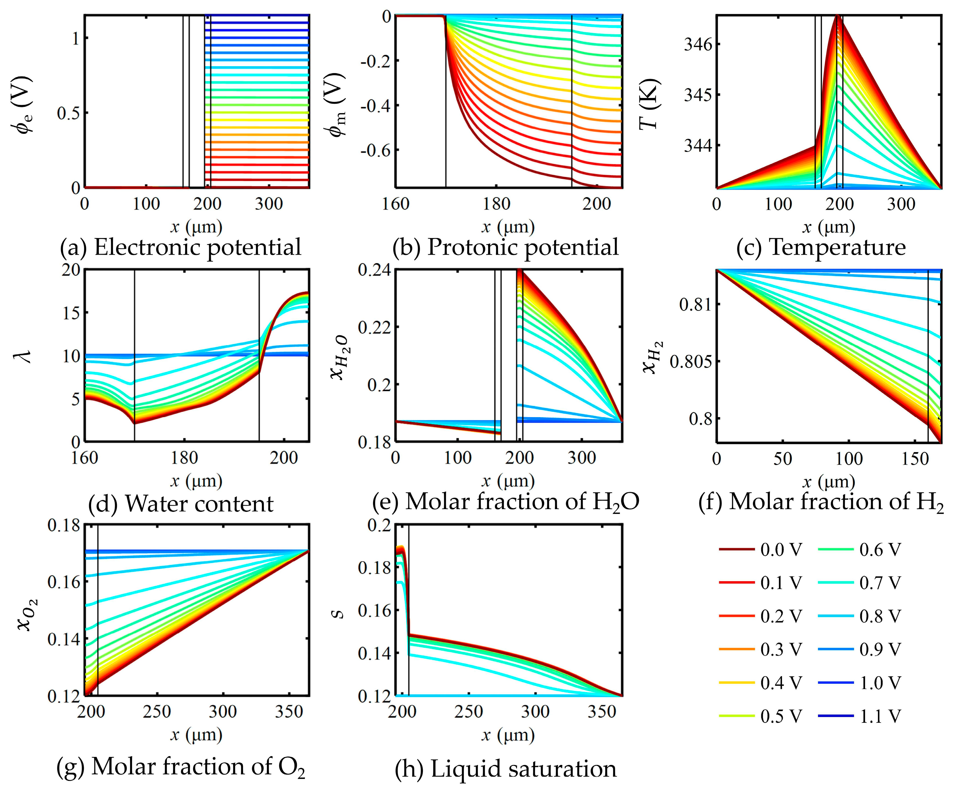
5.1. Distribution of Important Independent Variables Within the FC

Figure 6 shows the distribution of key variables of the FC under the optimal parameter combination. Each figure contains 24 lines, representing different V_cell values, starting from 1.15 V and decreasing by 0.05 V to 0 V. The corresponding V_cell values for different colors are shown in the legend, and for the sake of saving drawing space, only V_cell values changing at intervals of 0.1 V are plotted in the legend. The vertical lines in each subgraph serve to separate adjacent but distinct regions. Figure 6a shows the distribution of ϕ_e within the FC as V_cell decreases from 1.15 V to 0 V. Only the cathode side experiences a change in ϕ_e, while the anode remains at 0 V. As V_cell decreases, the current density (I) gradually increases, and the number of protons produced by hydrogen decomposition also increases, resulting in a gradual decrease in ϕ_m (an increase in absolute value), as shown in Figure 6b, and the direction of decrease is consistent with the direction of proton transmembrane transport. Due to the ORR occurring in the CCL, which releases a large amount of heat, the temperature distribution within the FC shown in Figure 6c has the highest point at the CCL and decreases towards both sides. Moreover, due to the different k values in each region, the rate of temperature decrease also varies. The larger the k value, the higher the heat transfer efficiency, the more uniform the temperature distribution, and the smaller the slope. By observing the slopes of temperature change in each region, it can be found that k_AGDL > k_CGDL > k_A/CCL > k_PEM, which is consistent with the actual situation. Through electroosmotic drag, protons in the form of hydrated hydrogen ions are transferred from the ACL to the CCL, resulting in a decrease in the λ value of the ACL and an increase in the λ values of the PEM and CCL, as shown in Figure 6d. And as I increases, the proton production increases, dragging more dissolved water.

The mole fraction distribution of gaseous water is shown in Figure 6e. Due to the transformation of gaseous water to dissolved water in the ACL, the gaseous water gradually decreases from the AGDL to the ACL. The ORR in the CCL generates water, resulting in the highest water vapor content inside. As I increases, more water is produced, and the water vapor content in the CCL also increases. The distribution of hydrogen in the anode porous layer is shown in Figure 6f. As V_cell decreases, the electrochemical reaction becomes more intense, and more hydrogen is consumed. The hydrogen content gradually decreases from the AGDL to the ACL, and the rate of decrease in the ACL gradually increases. The distribution of oxygen in Figure 6g is similar to that of hydrogen. The distribution of liquid water saturation (s) is shown in Figure 6h. Part of the water generated by the ORR in the CCL is converted to liquid water and then discharged through the CGDL to the GC. Therefore, the s value in the CCL is significantly higher than that in the CGDL, and there is a distinct s step at the CCL|CGDL interface. As I increases and more water is generated, the s value rapidly increases. The distribution trends in all these variables are consistent with reality, confirming the validity of the numerical model.

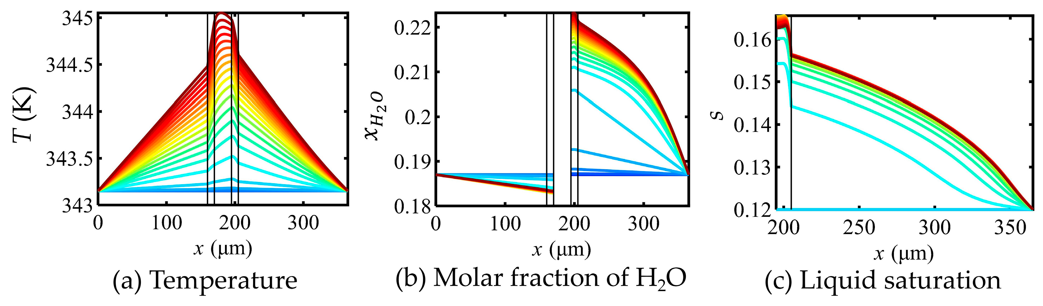
5.2. Effects of Mass Transfer Parameters on Key Variables in the FC

To study the influence of changes in mass transfer parameters on the transfer process within the FC, the distribution of important variables within the FC under the original mass transfer parameter combination was obtained through a numerical model. To save space, only the distribution of variables with significant changes is shown in Figure 7. By comparing Figure 7a with Figure 6c, the temperature distribution in Figure 7a is approximately symmetrical, gradually decreasing towards both GDLs with the PEM as the symmetry axis. Observing the temperature drop slopes in each region, it was found that k_A/CGDL > k_PEM > k_A/CCL. When V_cell ≥ 0.3 V, the highest temperature is at the PEM|CCL interface, but when V_cell < 0.3 V, the highest temperature is at the center of the PEM. The change in MEA-k can significantly affect the temperature distribution, which in turn affects the electrochemical reaction rate and the conversion rate of the water phase, thereby influencing the output performance of the FC. By comparing Figure 7b with Figure 6e, the water vapor content on the anode side is not significantly different, but the water vapor content on the cathode side decreases, and the rate of decrease towards the CGDL from the CCL gradually increases. From the calculation formula of the water vapor mole fraction, it mainly depends on the temperature on the cathode side. In the original case, the temperature on the cathode side is lower and more uniform, so P_sat is smaller, and more gaseous water is converted into dissolved water or liquid water. By comparing Figure 7c and Figure 6h, since I of the FC under the original parameter combination is smaller at the same V_cell, less water is generated by the reaction, so its s value is lower. The κ_CCL of the original case is greater than that of the optimal case, and the liquid water transfer is smoother, so the s value variation range within the CCL is smaller. However, the κ_CGDL of the original case is smaller than that of the optimal case, and the liquid water transfer is hindered, resulting in a larger variation range in the s value within it. This analysis indicates that the change in the mass transfer properties of the MEA can significantly alter the values and distributions of temperature, water vapor, and liquid water within the FC, thereby affecting its output performance.

5.3. Impact of Optimizing Mass Transfer Parameters on FC Performance

To compare the extent of the impact of optimizing the mass transfer parameters on P_d, the polarization curves and P_d curves of FC under the original parameter combination and the optimized parameter combination are plotted in Figure 8. The optimization of ${\mathit{\sigma }}_{\mathrm{e}}^{\mathrm{A}/\mathrm{C}\mathrm{C}\mathrm{L}}$ and ${\mathit{\sigma }}_{\mathrm{e}}^{\mathrm{A}/\mathrm{C}\mathrm{G}\mathrm{D}\mathrm{L}}$ slightly extended the ohmic polarization region of the FC, while the optimization of MEA-k and κ enhanced the transfer of reactants and products, accelerated the electrochemical reaction, and thus improved the performance of the concentration polarization region of the FC. The maximum P_d of the FC under the original parameter combination was 0.8705 W·cm⁻², whereas under the optimized combination, it reached 0.9184 W·cm⁻². The optimization of the attribute parameters increased the performance of the FC by 5.51%.

In the actual design of FCs, applying the optimization framework developed in this study can enhance cost-effectiveness through several aspects. (1) Optimization of computing resources. Compared with traditional 3D CFD models, the 1D parametric model reduces the simulation time from several hours to several seconds, while maintaining an error range within 3.87%. This enables rapid design iterations without the need for high-performance computing clusters. (2) Reduction in experimental costs. With the ANN surrogate model achieving a prediction accuracy of 99.85%, there is no need for extensive physical prototype iterative tests during the parameter optimization stage. Only experimental verification is required after optimization, which significantly reduces material consumption and testing costs. (3) Acceleration of the development cycle. This integrated framework can achieve multi-parameter optimization within seconds in each iteration, while traditional methods take several hours. This greater than 1000-fold speedup greatly shortens the timeline for design optimization. (4) Performance-driven cost savings. A 5.51% increase in net power density means that the reaction area of the FC can be reduced while maintaining equivalent output, thereby saving material costs.

6. Conclusions

Based on the established 1D parametric model, this study performed sensitivity analysis and global optimization of the MEA’s thermal and mass transfer properties by combining the ANN surrogate model and genetic algorithm, effectively enhancing the output performance of the FC. The main conclusions are as follows:

(1)

The 1D two-phase non-isothermal parametric model established in this study can capture the distribution of key variables within the FC and predict its output performance. Compared with the experimental results, the error was within 3.87%. Additionally, it requires minimal computational resources and time, demonstrating high practical value.

(2)

Sensitivity analysis revealed that k_PEM is negatively correlated with P_d, while other parameters are positively correlated. The parameter k_AGDL had the most significant impact on P_d, followed by k_CGDL, κ_GDL, ${\mathit{\sigma }}_{\mathrm{e}}^{\mathrm{A}\mathrm{G}\mathrm{D}\mathrm{L}}$, and ${\mathit{\sigma }}_{\mathrm{e}}^{\mathrm{C}\mathrm{G}\mathrm{D}\mathrm{L}}$. Remaining parameters exhibited negligible influence.

(3)

The ANN surrogate model achieved high accuracy, with the error between predicted and actual values remaining below 0.15%. When combined with the genetic algorithm, it could rapidly perform global optimization across multiple parameters within seconds, significantly improving the optimization efficiency.

(4)

The MEA’s mass transfer properties primarily affect the internal heat and mass transfer in the FC by influencing the temperature, gaseous water, and liquid water distributions. These adjustments improve the concentration polarization region, thereby enhancing electrochemical process and output performance.

(5)

The optimized mass transfer properties increased the net P_d of the FC by 5.51%. Through the combined optimization design process of the 1D model, ANN surrogate model, and genetic algorithm, an optimal solution can be obtained in a short time, which has certain reference significance for guiding the design process of the MEA.

References

1. Zuo, Q.; Wang, G.; Shen, Z.; Ma, Y.; Ouyang, Y.; Yang, D.; Lei, S.; Ouyang, M. Performance evaluation and field synergy analysis of PEMFC with novel snake coil flow field. Int. J. Heat Mass Transf. 2025, 238, 126470. [Google Scholar] [CrossRef]
2. Lee, S.H.; Nam, J.H.; Kim, C.J.; Kim, H.M. Numerical investigation of effective thermal conductivity of gas diffusion layer of the PEM fuel cell. Numer. Heat Transf. Part A Appl. 2024, 85, 1356–1378. [Google Scholar] [CrossRef]
3. Froning, D.; Wirtz, J.; Hoppe, E.; Lehnert, W. Flow Characteristics of Fibrous Gas Diffusion Layers Using Machine Learning Methods. Appl. Sci. 2022, 12, 12193. [Google Scholar] [CrossRef]
4. Xiao, L.; Yin, Z.; Bian, M.; Bevilacqua, N.; Zeis, R.; Yuan, J.; Sui, P. Microstructure reconstruction using fiber tracking technique and pore-scale simulations of heterogeneous gas diffusion layer. Int. J. Hydrog. Energy 2022, 47, 20218–20231. [Google Scholar] [CrossRef]
5. Ye, S.; Hou, Y.; Li, X.; Jiao, K.; Du, Q. Pore-Scale Investigation of Coupled Two-Phase and Reactive Transport in the Cathode Electrode of Proton Exchange Membrane Fuel Cells. Trans. Tianjin Univ. 2023, 29, 1–13. [Google Scholar] [CrossRef]
6. He, Y.; Bai, M.; Hao, L. Pore-Scale Simulation of Effective Transport Coefficients in the Catalyst Layer of Proton Exchange Membrane Fuel Cells. J. Electrochem. Soc. 2023, 170, 044501. [Google Scholar] [CrossRef]
7. Park, S.; Akbar, A.; Lee, J.; Kim, Y.; Um, S. Nanoscopic Post-Compression Effects on Transport Phenomena and Electrochemical Utilization in Quaternion Catalyst Layers for Fuel Cell Applications. Int. J. Precis. Eng. Manuf.-Green Technol. 2024, 11, 463–479. [Google Scholar] [CrossRef]
8. Chen, L.; Zhang, R.; Kang, Q.; Tao, W. Pore-scale study of pore-ionomer interfacial reactive transport processes in proton exchange membrane fuel cell catalyst layer. Chem. Eng. J. 2020, 391, 123590. [Google Scholar] [CrossRef]
9. Liu, Q.; Lan, F.; Chen, J.; Wang, J.; Zeng, C. Effect of anisotropic transport properties of porous layers on the dynamic performance of proton exchange membrane fuel cell. Int. J. Hydrog. Energy 2023, 48, 10982–11002. [Google Scholar] [CrossRef]
10. Zhang, G.; Qu, Z.; Yang, H.; Mu, Y.; Wang, Y. A one-dimensional model of air-cooled proton exchange membrane fuel cell stack integrating fan arrangement and operational characteristics. Appl. Therm. Eng. 2024, 249, 123353. [Google Scholar] [CrossRef]
11. Trinh, D.H.; Kim, Y.; Yu, S. One-dimensional dynamic model of a PEM fuel cell for analyzing through-plane species distribution and irreversible losses under various operating conditions. Case Stud. Therm. Eng. 2024, 60, 104815. [Google Scholar] [CrossRef]
12. Ding, Y.; Xu, L.; Zheng, W.; Hu, Z.; Shao, Y.; Li, J.; Ouyang, M. Characterizing the two-phase flow effect in gas channel of proton exchange membrane fuel cell with dimensionless number. Int. J. Hydrog. Energy 2023, 48, 5250–5265. [Google Scholar] [CrossRef]
13. Khemili, F.; Najjari, M. Numerical Modeling of the Influence of Gas Diffusion Layer Properties on Liquid Water Transport and Transient Responses in a Proton Exchange Membrane Fuel Cell. Microgravity Sci. Technol. 2023, 35, 42. [Google Scholar] [CrossRef]
14. Liu, Q.; Lan, F.; Wang, J.; Chen, Y.; Chen, J. Multi-objective optimization of helical baffle flow field structure for fuel cell under multiple performance indicator constraints. Renew. Energy 2025, 241, 122349. [Google Scholar] [CrossRef]
15. Zhang, Y.; Zhang, D.; Chen, Q.; Zhang, Y.; Jiang, X.; Yang, X.; Cao, J.; Deng, Q.; Chen, B.; Liu, Q.; et al. Three-dimensional full-morphology numerical simulation of PEM fuel cells: Spatial distribution characteristics of “gas–water-electricity” considering circular dot matrix gas distribution zones. Chem. Eng. J. 2025, 505, 159199. [Google Scholar] [CrossRef]
16. Neyerlin, K.C.; Gu, W.; Jorne, J.; Gasteiger, H.A. Determination of Catalyst Unique Parameters for the Oxygen Reduction Reaction in a PEMFC. J. Electrochem. Soc. 2006, 153, A1955. [Google Scholar] [CrossRef]
17. Neyerlin, K.C.; Gu, W.; Jorne, J.; Gasteiger, H.A. Study of the Exchange Current Density for the Hydrogen Oxidation and Evolution Reactions. J. Electrochem. Soc. 2007, 154, B631. [Google Scholar] [CrossRef]
18. Vetter, R.; Schumacher, J.O. Free open reference implementation of a two-phase PEM fuel cell model. Comput. Phys. Commun. 2019, 234, 223–234. [Google Scholar] [CrossRef]
19. Liu, Q.; Lan, F.; Chen, J.; Wang, J.; Zeng, C. Flow field structure design modification with helical baffle for proton exchange membrane fuel cell. Energy Convers. Manag. 2022, 269, 116175. [Google Scholar] [CrossRef]
20. Liu, Q. Study of Diffusion Layer Pore Characteristics and Helical Baffle Flow Field Improvement for Fuel Cell Mass Transfer Capability Enhancement. Ph.D. Thesis, South China University of Technology, Guangzhou, China, 2023. [Google Scholar]
21. Weber, A.Z.; Borup, R.L.; Darling, R.M.; Das, P.K.; Dursch, T.J.; Gu, W.; Harvey, D.; Kusoglu, A.; Litster, S.; Mench, M.M.; et al. A Critical Review of Modeling Transport Phenomena in Polymer-Electrolyte Fuel Cells. J. Electrochem. Soc. 2014, 161, F1254. [Google Scholar] [CrossRef]
22. Raghunath, K.V.; Reddy, B.K.; Muliankeezhil, S.; Aparna, K. Non-isothermal One-Dimensional Two-Phase Model of Water Transport in Proton Exchange Membrane Fuel Cells with Micro-porous Layer. Arab. J. Sci. Eng. 2023, 48, 8543–8556. [Google Scholar] [CrossRef]
23. Zhao, G.; Liu, H.; Sun, H.; Hu, Z.; Li, J.; Xu, L.; Ouyang, M. Analysis and Optimization of Commercial Scale PEMFCs with Different Flow Channels Prepared by Ultrafast Laser Fabrication Technique. Automot. Innov. 2024, 7, 225–235. [Google Scholar] [CrossRef]
24. Tao, J.; Wei, X.; Ming, P.; Wang, X.; Jiang, S.; Dai, H. Order reduction, simplification and parameters identification for cold start model of PEM fuel cell. Energy Convers. Manag. 2022, 274, 116465. [Google Scholar] [CrossRef]
25. Li, Y.; Yang, Z.; Ji, X.; Liu, F.; And Hao, D. Sensitivity analysis of structural parameters for PEMFCs based on 1D transient model and elementary effect method. Int. J. Green Energy 2024, 21, 87–101. [Google Scholar] [CrossRef]
Figure 1. Geometric structure of the fuel cell with a five-layer membrane electrode model (not to scale).
Energies 18 02414 g001
Figure 2. (a) Experimental equipment diagram and (b) validation of the research results.
Energies 18 02414 g002
Figure 3. Sensitivity of power density to variations in research parameters.
Energies 18 02414 g003
Figure 4. Flowchart showing the optimization design used in this study.
Energies 18 02414 g004
Figure 5. Training status of the neural network model.
Energies 18 02414 g005
Figure 6. Distribution curves of various key variables in the through-plane direction at different voltages.
Energies 18 02414 g006
Figure 7. Distribution curves of various variables at different voltages under the original parameter combination.
Energies 18 02414 g007
Figure 8. Comparison of the FC polarization and Pd curves under the best and original mass transfer parameter combinations.
Energies 18 02414 g008