Interpretable Combinatorial Machine Learning-Based Shale Fracability Evaluation Methods

Abstract

Shale gas, as an important unconventional hydrocarbon resource, has attracted much attention due to its great potential and the need for energy diversification. However, shale gas reservoirs with low permeability and low porosity pose challenges for extraction, making shale fracability evaluation crucial. Conventional methods have limitations as they cannot comprehensively consider the effects of non-linear factors or quantitatively analyse the effects of factors. In this paper, an interpretable combinatorial machine learning shale fracability evaluation method is proposed, which combines XGBoost and Bayesian optimization techniques to mine the non-linear relationship between the influencing factors and fracability, and to achieve more accurate fracability evaluations with a lower error rate (maximum MAPE not more than 20%). SHAP(SHapley Additive exPlanation) value analyses were used to quantitatively assess the factor impacts, provide the characteristic importance ranking, and visualise the contribution trend through summary and dependency plots. Analyses of seven scenarios showed that ‘Vertical—Min Horizontal’ and ‘Vertical Stress’ had the greatest impact. This approach improves the accuracy and interpretability of the assessment and provides strong support for shale gas exploration and development by enhancing the understanding of the role of factors.

1. Introduction

Shale gas, as a crucial unconventional hydrocarbon resource, has gained significant attention in recent years due to its vast potential and the need to diversify energy sources globally. With the increasing demand for energy and the depletion of conventional oil and gas reserves, the exploration and development of shale gas have become increasingly important for ensuring energy security and reducing reliance on imports [1].

Shale gas reservoirs, characterized by low permeability and porosity, pose significant challenges in their efficient exploitation [2]. To unlock the trapped gas within these formations, hydraulic fracturing techniques are commonly employed to create artificial fractures in the shale rock. The success of hydraulic fracturing is strongly influenced by the fracability of the shale, which refers to its ability to be fractured effectively [3]. Therefore, evaluating the fracability of shale gas reservoirs is of paramount importance in optimizing drilling and completion strategies, enhancing gas production rates, and reducing operational costs.

In order to evaluate the fracturability of reservoirs, two experimental evaluation and comprehensive evaluation methods have been developed. The experimental evaluation [4] directly observes whether a complex network of hydraulic fractures is formed in the core samples through indoor hydraulic fracturing physical simulation experiments, and then determines the fracturability of the reservoir. The experimental simulation method is a complex and time-consuming process. Only a few dispersed points can be obtained at the same time, so it is difficult to use this method on a large scale in the field [5].

The integrated evaluation method uses the continuity of logging data to obtain a continuous brittle profile. Since there is no specific evaluation index and measurement method in rock mechanics, scholars in different fields have proposed different definitions and calculation methods according to different evaluation purposes. Wu et al.’s quantitative evaluation of shale fracture ratio with brittleness, quartz content, diagenesis, and natural fracture as the main fracability related factors [5] determined the weighting coefficients of the brittleness contribution of different minerals such as pyrite, dolomite, calcite, feldspar, and clay minerals using quartz as the standard brittle mineral and calculated the overall brittleness of the shales [6]. In addition, some other scholars have used brittle mineral content to calculate the fracturing index [7]. More and more studies have realized that fracability depends not only on the brittleness of the material, but also on some other factors such as diagenesis, ductility, natural fracture, tensile strength, etc., and some quantitative methods of rock fragmentation have been proposed to incorporate these factors [8,9,10]. Despite the increasing number of factors taken into account, comprehensive evaluation methods are still mainly based on linear equations and simpler non-linear equation evaluation methods. This approach makes it difficult to analyse complex non-linear interactions. And because there are so many evaluation methods, it is difficult to choose an appropriate one.

The above study shows that traditional shale fracability is only evaluated by establishing a linear evaluation model through some specific influencing factors to evaluate the fracability of shale. However, the evaluation of shale fracability is a complex process involving a variety of factors, such as rock brittleness, mineral composition, diagenesis, and the presence of natural fractures. These factors interact with each other in a nonlinear manner, and traditional evaluation models are unable to comprehensively consider the nonlinear effects of each factor on fracability. At the same time, it is also impossible to quantitatively analyse the effects of various factors on fracability. In recent years, with the development of artificial intelligence, machine learning methods have excelled in mining nonlinear relationships between data [11], methods such as Support Vector Machine (SVM) [12], Autoencoder [13], and XGBoost [14]. For example, Hui et al., used a machine learning approach to mine the fly-linear relationship between two factors, geological and operational, and shale gas production to achieve accurate shale gas production predictions [15]. XGBoost has strong learning ability and has been widely used in various fields. In order to construct machine learning models with superior performance, numerous researchers have actively explored and adopted various optimization strategies, including genetic algorithms, grid search methods, and Bayesian optimization algorithms [16,17]. Among these optimization algorithms, the Bayesian optimization algorithm stands out as a high-profile choice due to its excellent search efficiency. Meanwhile, the field of interpretable machine learning has also seen rapid development with the advancement of technology, and those methods that can deeply analyse the impact of input features on the output results, such as SHAP value, are, especially, gaining more and more attention.

In summary, we propose an interpretable combinatorial machine learning-based shale fracability evaluation method. In this method, first, we establish a shale compressibility evaluation model based on XGBoost and mine the nonlinear relationship between influencing factors and compressibility evaluation indexes to achieve compressibility evaluation. Second, a Bayesian optimization algorithm is introduced to optimise the model with hyperparameters to obtain the optimal model. Finally, the effects of different influencing factors on fracability are analysed using SHAP values [18,19].

The contributions of this paper are as follows:

(1)

Propose to use a combined machine learning model combining a Bayesian optimization algorithm and XGBoost to mine the non-linear relationship between different influencing factors and shale fracability.

(2)

It is proposed to use the SHAP value to quantitatively analyse the effects of different influencing factors on shale fracability.

2. Methodology

Our proposed method uses the XGBoost model to mine the nonlinear relationship between the influencing factors and the fracability indexes, and adjusts the model parameters with the Bayesian optimization method to achieve the automated calculation of the fracability indexes with the influencing factors and complete the fracability evaluation. Finally, the SHAP value method is introduced to explain the role of influencing factors in calculating the fracability index.

2.1. Non-Linear Relationship Mining

XGBoost is an emerging and efficient integrated model [20]. Its base learner is CART (Classification and Regression Tree). A single CART [21,22] consists of multiple leaf nodes. During the training and application of the model, for a defined set of input data, there exists a leaf node output value corresponding to it. The multiple leaf nodes of a single CART comprehensively characterise the prediction result of that CART for the current input data. Based on this, the XGBoost model takes the sum of the predicted values of all CARTs for a sample as the output value for that sample, calculated as in Equations (1) and (2):

$${\widehat{y}}_i=\varphi \left(x_i\right)={\displaystyle \sum _{k=1}^K{f}_k}\left(x_i\right),\hspace{1em}{f}_k\in \mathcal{F}$$

(1)

$$\mathcal{F}=\left\{f(x)=w_{q(x)}\right\}\left(q:R^m\to T,w\in R^T\right)$$

(2)

where ${\widehat{y}}_i$ is the model prediction, $x_i$ is the ith sample, $f_k$ is the kth tree model, $\mathcal{F}$ is the space of the decision tree, m is the number of features, T is the number of leaf nodes of each tree, q is the fraction of each sample mapped by the structure of each tree to the corresponding leaf node, i.e., q denotes the model of the tree, which inputs a sample and outputs a predicted fraction of the samples to the leaf nodes according to the model mapped to the leaf nodes, and $w_{q(x)}$ is the fraction of all leaf nodes of the tree q. The scores form a set.

2.2. Model Tuning

Bayesian optimization [23] is generally used to solve single-objective optimization problems, i.e., $x^{*}={\mathrm{argmin}}_{x\in \mathrm{\Omega }}y(x)$, where $x^{*}=(x_1,x_2,\dots ,x_d)$ is a d-dimensional hyperparameter variable, $\mathrm{\Omega }$ is the parameter space to which $x^{*}$ belongs, and $y(•)$ is the objective function. Bayesian optimization is an effective method for solving black-box function optimization problems. It primarily consists of two key components: first, constructing a probabilistic surrogate model based on the observed sample set to infer the posterior probability distribution of the target black-box function; second, constructing an acquisition function based on the posterior probability distribution, and determining the next sampling point by maximizing the acquisition function. The newly sampled data is then used to augment the dataset and update the probabilistic surrogate model. Through an iterative process, Bayesian optimization employs model-based sequential optimization to search for the optimal solution of the objective function $y(•)$. The basic workflow is outlined as follows:

(1)

Initialise n parameter vectors $X=\{x_1,x_2,\dots ,x_n\}$, and then for each parameter vector obtain the return value $y=\{y_1,y_2,\dots ,y_n\}$ corresponding to the objective function;

(2)

Fit a probabilistic agent model based on the already observed data set {X,y} and infer the posterior distribution of the objective function;

(3)

Calculate a collection function based on the posterior distribution obtained in step (2), and select the next sampling point to sample by maximizing the collection function;

(4)

Go back to step (2) and keep updating the probabilistic agent model iteratively until the termination condition is satisfied and then stop the iteration.

In Bayesian optimization, the essence lies in the initialization of the sampling set, the establishment of the probabilistic surrogate model, and the choice of the acquisition function. The probabilistic surrogate model serves to fit the existing dataset, inferring the probability distribution of the objective function. Meanwhile, the acquisition function selects the subsequent sampling point based on the current distribution, thereby transforming the costly-to-evaluate and non-explicitly solvable black-box function optimization problem into an explicitly solvable optimization problem of the acquisition function.

2.2.1. Initializing the Sample Set

Latin hypercube sampling is commonly used in Bayesian optimization to initialise the sampling set (LSH), and LHS is a stratified random sampling method capable of efficiently sampling from a multivariate distribution interval. Assuming that there are now d variables $X=\{x_1,x_2,\dots ,x_n\}$, from which N samples are taken in a specified interval, then an initial sampling set of N sample points is generated according to the following: Suppose $A_{N\times d}=(a_{ij})$, each of whose columns is a random permutation of the set $F_n=\{1,\dots ,N\}$. Let $x_{ij}={\displaystyle \frac{a_{ij}-k_{ij}}{N}},i=1,\dots ,N,j=1,\dots ,d$, where k_ij are all a random number generated on the distribution $U(0,1)$. Then the $M_{N\times d}=(x_{ij})$ matrix constitutes the initial sampling set for Bayesian optimization, and each row in the matrix represents a sampling point. The LHS makes the initial sampling set spatially populated to avoid the algorithm falling into a local optimum solution due to the influence of initialised sampling during the Bayesian optimization process.

2.2.2. Agent Models Based on Gaussian Processes

Agent models are generally probabilistic models in non-parametric form, such as Gaussian processes. Gaussian processes are extensions of multivariate Gaussian distributions to infinite dimensional stochastic processes. The stochastic process depends on its mean function ${\mu }_0(•)$ and variance function ${\delta }_0(•)$. Given a sample x_n, it returns a conditional probability based on x_1:n−1 with respect to f(x), which is generally referred to as the posterior probability, and obeys a Gaussian distribution with a given mean and variance:

$$f\left(x_n\right)\mid f\left(x_{1:n-1}\right)~GP\left({\mu }_n\left(x_n\right),{\sigma }_n^2\left(x_n\right)\right)$$

(3)

$${\mu }_n\left(x_n\right)={\mathrm{\Sigma }}_0\left(x_n,x_{1:n-1}\right){\mathrm{\Sigma }}_0{\left(x_{1:n-1},x_{1:n-1}\right)}^{-1}\left(f\left(x_{1:n-1}\right)-{\mu }_0\left(x_{1:n-1}\right)\right)+{\mu }_0\left(x_n\right)$$

(4)

$${\sigma }_n^2\left(x_n\right)={\mathrm{\Sigma }}_0\left(x_n,x_n\right)-{\mathrm{\Sigma }}_0\left(x_n,x_{1:n-1}\right){\mathrm{\Sigma }}_0{\left(x_{1:n-1},x_{1:n-1}\right)}^{-1}{\mathrm{\Sigma }}_0\left(x_{1:n-1},x_n\right)$$

(5)

To obtain the analytical solution of the posterior probability distribution, it is also necessary to determine the form of the mean and variance functions (kernel functions). In Gaussian processes, the mean function is often assumed ${\mu }_0=0$, which simplifies the form of the posterior probability distribution; the kernel function mainly determines the shape of the posterior probability distribution and also ultimately determines the properties that the agent model has. The kernel function acts on all sample points $x_i,y_i\in {ℝ}^n$ in the form of two pairs, returning scalars representing the similarity between the two points, which are used to describe the interactions between $x_i$ and $y_i$. All of these scalars form the covariance matrix $\sum$ of the posterior probability distribution. Gaussian kernel and Matérn kernel are commonly used as kernel function in Gaussian process, and the expression of Gaussian kernel function is shown in Equation (6)

$${\mathrm{\Sigma }}_0\left(x,x^{\prime }\right)={\sigma }_f^2\exp \left(-{\displaystyle \frac{1}{2l^2}}{\left(x-x^{\prime }\right)}^T\left(x-x^{\prime }\right)\right)$$

(6)

where ${\sigma }_f$ and l are parameters of the Gaussian kernel function, the l parameter controls the smoothness of the function, and the ${\sigma }_f$ parameter controls the vertical variation of the function.

2.2.3. Acquisition Functions

The acquisition function is used to guide the location of the next sampling point in Bayesian optimization. EI (Expected Improvement) is often used as the acquisition function.

Let $f^{*}=\min \left\{f\left(x_1\right),\dots ,f\left(x_n\right)\right\}$ be the optimal value of the objective function in a known sample, the EI acquisition function finds the next sampling point Y by quantifying the expectation of the lift of the sample point x to the current optimal value of the objective function, as in Equation (7). The EI acquisition function is shown in Equation (8)

$$I(x)=\max \left(Y-f^{*},0\right)$$

(7)

$$EI(x)=\left(\mu -f^{*}\right)\mathrm{\Phi }\left({\displaystyle \frac{\mu -f^{*}}{\sigma }}\right)+\sigma \varphi \left({\displaystyle \frac{\mu -f^{*}}{\sigma }}\right)$$

(8)

where $\varphi (•)$ and $\mathrm{\Phi }(•)$ are the probability density function and cumulative distribution function of the Gaussian distribution, respectively.

2.2.4. Optimise Hyperparameter Settings

As in

Table 1. Hyperparameter tuning.

Hyperparameters	Values
Max_depth	[3, 50]
Num_leaves	[50, 300]
Learning_rate	[0.001, 0.08]

, we set 3 hyperparameters Max_depth, Num_leaves, and Learning_rate and optimise them using this method.

2.3. Quantitative Analysis of Impact Factors

SHAP value [24] analysis is a method for interpreting the prediction results of machine learning models, where the core idea lies in calculating the marginal contribution of features to the model output. The SHAP value is derived from cooperative game theory and is used to measure the contribution of features to the model prediction results. For each prediction sample, the model generates a prediction value, and the SHAP value is the value assigned to each feature in that sample. Specifically, SHAP value analysis interprets the values assigned to each feature in the prediction sample by constructing an additive explanatory model that treats each feature as a ‘contributor’. These values represent the extent to which each feature contributes to the prediction. By calculating the SHAP value for each feature, we can understand the importance and influence of the feature in the model prediction. In SHAP value analyses, when the SHAP value of a feature is greater than 0, it means that the feature enhances the prediction; conversely, it means that the feature makes the prediction lower.

Traditional feature importance only tells which feature is important, but we don’t know how that feature affects the prediction results. The biggest advantage of SHAP’s value is that SHAP’s value can reflect the influence of each feature in the sample and also show the positive and negative influence. The goal of the SHAP value is to explain the results of the model judgement by calculating the contribution of each feature in the input data to the model prediction.

2.4. Baseline Model

2.4.1. Autoencoder

An Autoencoder is an unsupervised learning neural network model. It is designed to learn latent feature representations of input data [25]. This is achieved through compression and reconstruction. The model consists of two main parts: an Encoder and a Decoder. The Encoder maps the input data into a low-dimensional latent space [26]. The Decoder reconstructs the output data from this latent space. The goal is to make the output as close as possible to the input.

The working principle of an Autoencoder can be summarized in three steps:

(1)

Encoding Stage

The Encoder compresses high-dimensional input data into a low-dimensional latent space. This is done through a series of nonlinear transformations. The goal is to extract the main features of the input data. The mathematical expression is as follows:

$$h=f\left(W\_\left\{enc\right\}x+b\_\left\{enc\right\}\right)$$

(9)

where, x is the input data, W_enc and b_enc are the weights and biases of the encoder, respectively, and f is the activation function.

(2)

Decoding Stage

The Decoder reconstructs the data from the low-dimensional latent space. The goal is to make the reconstructed data as similar as possible to the original input. The mathematical expression is as follows:

$$\widehat{x}=g(W_{dec}h+b_{dec})$$

(10)

where, $\widehat{x}$ represents the reconstructed data, W_dec and b_dec are the weights and biases of the Decoder, respectively, and g is the activation function.

2.4.2. Kernel SVM

Kernel SVM is an extended version of Support Vector Machine (SVM) that addresses nonlinear problems by utilizing kernel functions [27]. Traditional linear SVMs are limited in handling nonlinear data. Kernel SVM solves this by mapping data into a higher-dimensional space, where originally non-separable data becomes linearly separable [28].

Kernel SVM is powerful due to its flexibility and generality, making it highly effective in solving nonlinear classification and regression problems.

2.5. Evaluation Indicators

We used three evaluation metrics, MAE (Mean Absolute Error), RMSE (Root Mean Squared Error), and MAPE (Mean Absolute Percentage Error) to judge the merits of the shale fracability evaluation model. In Equations (11)–(13).

$$\mathrm{MAE}={\displaystyle \frac{1}{n}}{\displaystyle \sum _{i=1}^n\left|{y_i}^{\prime }-y_i\right|}$$

(11)

$$\mathrm{RMSE}=\sqrt{{\displaystyle \frac{1}{n}}{\displaystyle \sum _{i=1}^n({y_i}^{\prime }-y_i}{)}^2}$$

(12)

$$\mathrm{MAPE}={\displaystyle \frac{1}{n}}{\displaystyle \sum _{i=1}^n\left|\frac{{y_i}^{\prime }-y_i}{y_i}\right|}\times 100\%$$

(13)

n is the number of samples, y_i denotes the sample true value, ${y_i}^{\prime }$ denotes the model output value, and ȳ_i denotes the average of the sample true values.

3. Case Study

3.1. Data Description

This section uses data from one company for the case study. This dataset has ‘Minimum Horizontal Stress’, ‘Maximum Horizontal Stress’, ‘Max Horizontal—Min Horizontal’, ‘Vertical Stress’, ‘Vertical—Min Horizontal’, ‘Elasticity Modulus’, ‘Poisson’s Ratio’, ‘Fracturing Fluid Viscosity’, ‘Flow Rate’, and 9 fracability influencing factors. At the same time, there are ‘Total Fracture Area’, ‘Natural Fracture Area’, ‘Main Fracture Area’, ‘Ratio Of Natural Fracture To Main Fracture Area’, ‘Main Fracture Width’, ‘Main Fracture Length’, and ‘Main Fracture Height’.

The dataset has a total of 800 sets of data samples, and the division ratio of training set, validation set, and test set is 6:2:2. In order to reduce the overfitting problem, we introduced an early stopping mechanism based on the validation set data.

3.2. Evaluation of Shale Fracability

We take the influencing factors as the input parameters of the model and the fracability evaluation indexes as the output parameters. We designed 7 sets of comparison experiments for 7 fracability indicators, respectively. In the experiments, we use MAE, RMSE, and MAPE as the evaluation indexes of the model. The lower the value of these three indicators, the better the model effect. In this subsection, we use Kernel SVM with Autoencoder as baseline models to verify the effectiveness of the overall approach.

Table 2. Accuracy of ‘Total Fracture Area’ calculation.

Models	MAE	RMSE	MAPE, %
Autoendcoder	5.3	1.99	3.4
Kernel SVM	5.1	1.67	3.0
Bayesian-XGBoost	4.24	1.52	2.7

,

Table 3. Accuracy of ‘Natural Fracture Area’ calculation.

Models	MAE	RMSE	MAPE, %
Autoendcoder	5.1	2.4	13
Kernel SVM	4.5	1.49	11
Bayesian-XGBoost	4.46	1.44	8

,

Table 4. ‘Main Fracture Area’ calculation accuracy.

Models	MAE	RMSE	MAPE, %
Autoendcoder	4.5	2.4	5.6
Kernel SVM	3.4	1.4	4.5
Bayesian-XGBoost	1.18	0.4	2.23

,

Table 5. ‘Ratio Of Natural Fracture To Main Fracture Area’ calculation accuracy.

Models	MAE	RMSE	MAPE, %
Autoendcoder	0.94	0.37	27.88
Kernel SVM	0.83	0.32	24.31
Bayesian-XGBoost	0.78	0.28	19.21

,

Table 6. Accuracy of ‘Main Fracture Width’ calculation.

Models	MAE	RMSE	MAPE, %
Autoendcoder	0.00031	0.00028	8.23
Kernel SVM	0.00023	0.00022	7.32
Bayesian-XGBoost	0.00017	0.00011	6.18

,

Table 7. Accuracy of ‘Main Fracture Length’ calculation.

Models	MAE	RMSE	MAPE, %
Autoendcoder	0.47	0.31	4.9
Kernel SVM	0.35	0.26	4.4
Bayesian-XGBoost	0.27	0.12	2.3

and

Table 8. ‘Main Fracture Height’ calculation accuracy.

Models	MAE	RMSE	MAPE, %
Autoendcoder	0.51	0.77	1.96
Kernel SVM	0.45	0.71	1.78
Bayesian-XGBoost	0.39	0.68	1.52

demonstrates the calculation accuracy of the fracability evaluation indexes of different methods, and the optimal methods are shown in bold form. Table 2, Table 3, Table 4, Table 5, Table 6, Table 7 and Table 8 shows that our proposed method has high accuracy in calculating the fracability evaluation indexes and can achieve a more accurate evaluation.

Cross-validation was performed to verify the robustness of our proposed method. We disrupted the data 5 times and divided the dataset in 6:2:2. As shown in

Table 9. Cross-validation.

	Evaluation Metrics	1	2	3	4	5
Scenario 1	RMSE	1.62	1.94	2.21	1.6	1.95
	MAPE%	2.26	2.41	2.96	2.52	2.68
Scenario 2	RMSE	1.34	1.23	1.42	1.79	1.55
	MAPE%	7.22	5.03	5.56	8.92	5.14
Scenario 3	RMSE	0.53	0.63	0.59	0.64	0.47
	MAPE%	4.51	3.42	3.39	3.4	2.54
Scenario 4	RMSE	0.23	0.27	0.32	0.29	0.39
	MAPE%	12.36	11.73	6.78	6.61	8.76
Scenario 5	RMSE	0.00013	0.00011	0.00011	0.00012	0.00013
	MAPE%	5.79	5.18	5.75	5.91	6.5
Scenario 6	RMSE	0.16	0.15	0.13	0.15	0.17
	MAPE%	2.9	2.7	3.07	3.31	3.62
Scenario 7	RMSE	0.48	0.55	0.87	0.28	0.49
	MAPE%	1.63	1.14	2.45	0.58	1.92

, the highest MAPE for the five tests is 12.36%, based on no more than 20%. This result shows that our method has some stability.

3.3. Analysis of Impact Factors

(1)

Scenario 1: The Total Crack Area

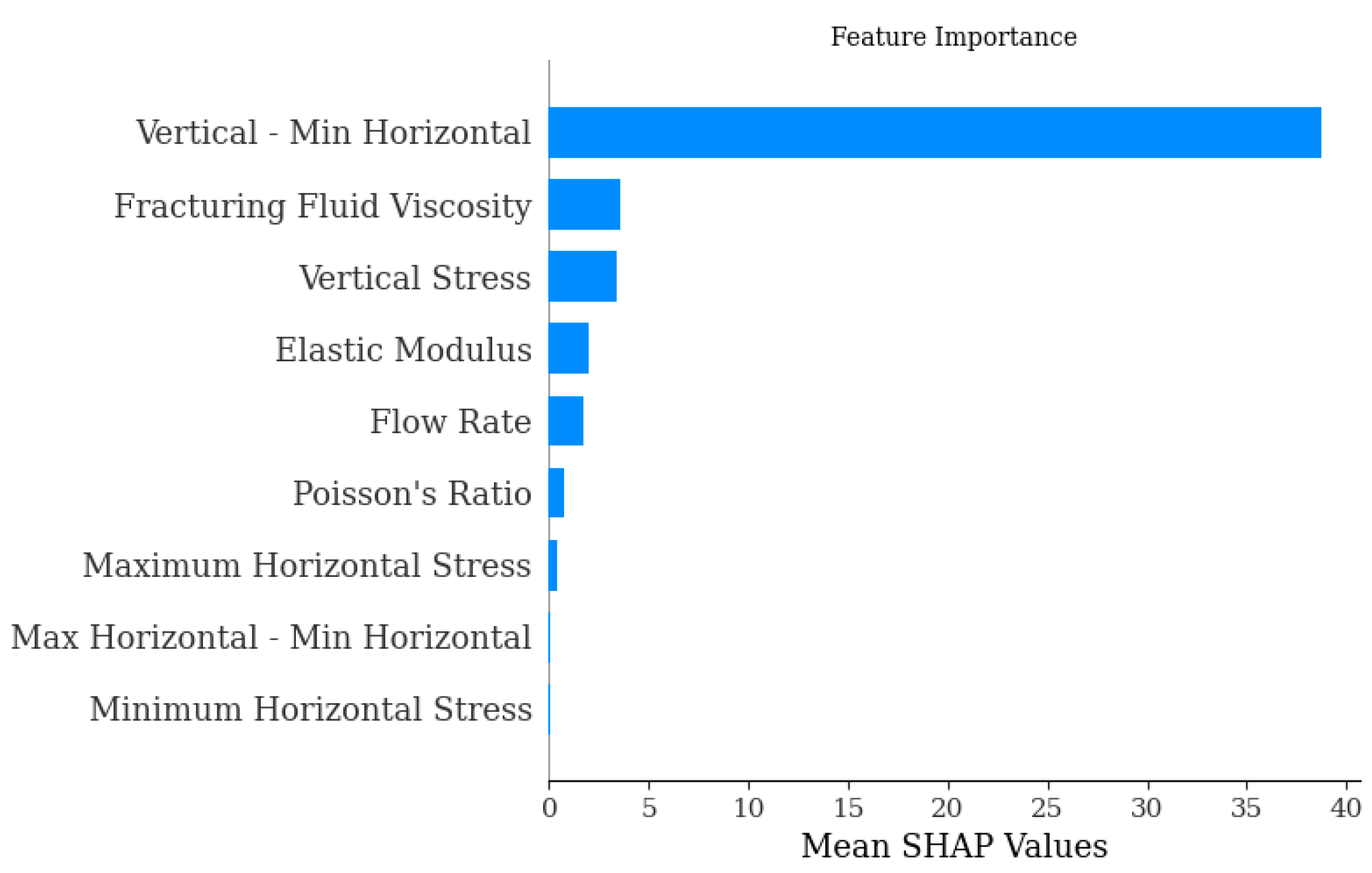
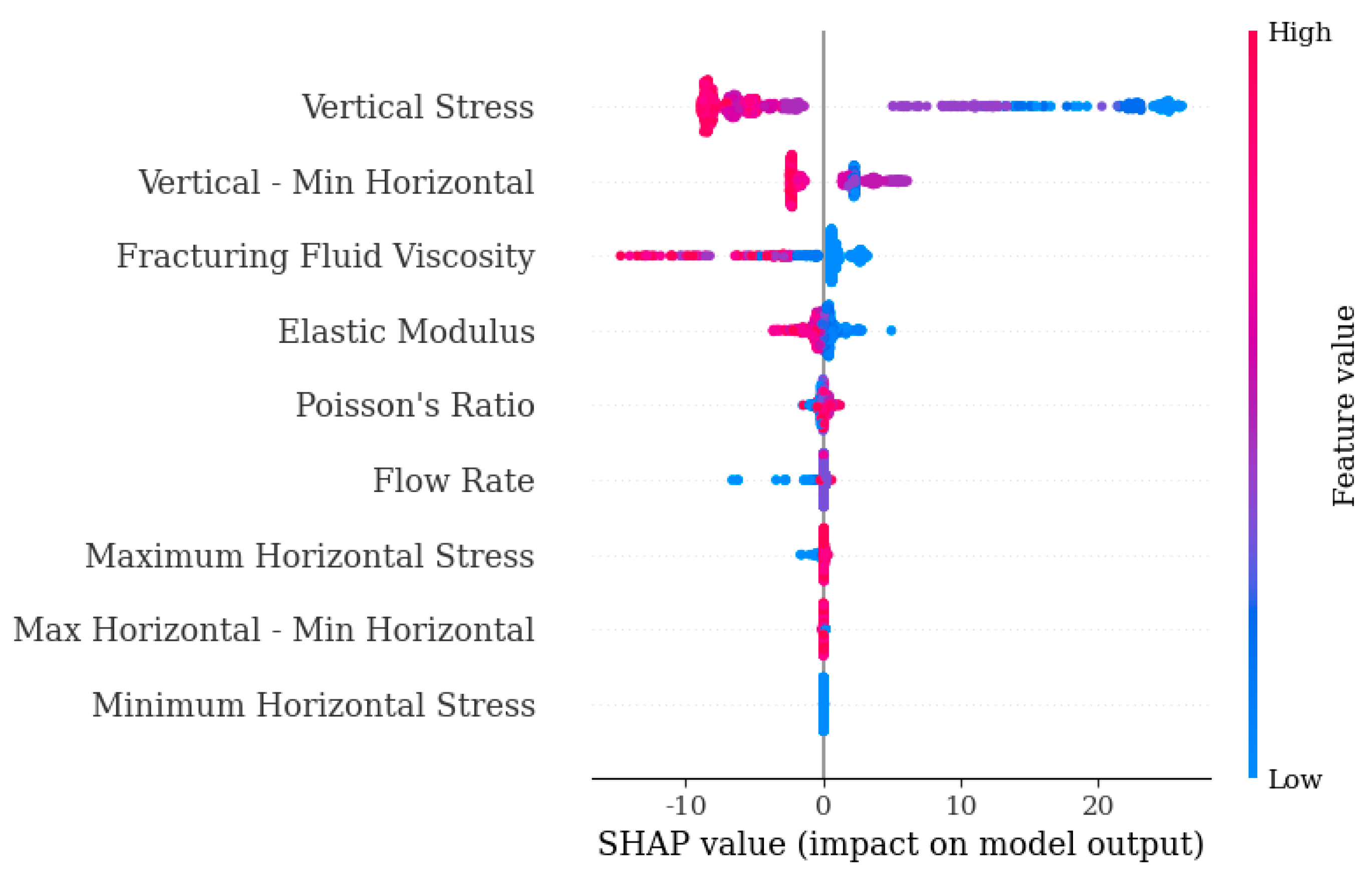
For example, in Figure 1, the importance of each feature decreases downward along the vertical axis. In Figure 2, the importance of features on the left side of the Summary diagram decreases from top to bottom, and the order of importance in Figure 2 is consistent with that in the Figure 1. The larger the value of a feature on the right side of the figure, the redder the colour. The Dependence diagram in Figure 3 mainly reflects the relationship between a certain feature and its SHAP value, showing the trend of change in the SHAP value as the feature value changes.

The analysis of Figure 1 and Figure 2 shows that the “Vertical—Min Horizontal”, i.e., the difference between the Vertical Stress and the horizontal minimum stress, has the greatest influence on the total crack area and far exceeds the influence of the other features on the prediction results. Therefore, the “Vertical—Min Horizontal” feature is analysed separately.

Next, we analyse ‘Vertical—Min Horizontal’. Looking at Figure 2, we can see that the larger SHAP values of this influence factor are mostly distributed in the negative direction. This phenomenon indicates that the influence factor is more likely to be negative in this scenario. However, there are cases where the factor has a smaller value when the SHAP value is negative, and similarly when the SHAP value is positive. This result shows that there is a threshold value that shifts the positive and negative influence of the factor.

As shown in Figure 3, the SHAP value changes significantly when ‘Vertical—Min Horizontal’ is 5. When the value is greater than 5, the SHAP value is negative, which means that when the eigenvalue is greater than 5, the factor has a negative effect on the total crack area. When the eigenvalue is less than 5, it is a positive influence.

(2)

Scenario 2: The Area of Natural Cracks

The analysis of Figure 4 and Figure 5 shows that the “Vertical—Min Horizontal”, i.e., the difference between the Vertical Stress and the horizontal minimum stress, has the greatest influence on the natural crack area and far exceeds the influence of the other features on the prediction results. Therefore, the “Vertical—Min Horizontal” feature is analysed separately.

Next, we analyse ‘Vertical—Min Horizontal’. Looking at Figure 5, we can see that the larger SHAP values of this influence factor are mostly distributed in the negative direction. This phenomenon suggests that the influence factor is more likely to be negative in this scenario. However, there are also cases where the factor has a small value when the SHAP is negative, and a similar phenomenon exists when the SHAP is positive. This result shows that there is a threshold value that shifts the positive and negative influence of the factor.

As shown in Figure 6, the SHAP value changes significantly to positive and negative values at a value of 5 for this factor. When the value of this factor is greater than 5, the SHAP value becomes negative. This phenomenon illustrates that the factor has a positive effect when the eigenvalue is less than 5 and a negative effect when the eigenvalue is greater than 5.

(3)

Scenario 3: The Main Crack Area

The analysis of Figure 7 shows that the “Vertical—Min Horizontal”, i.e., the difference between the Vertical Stress and the horizontal minimum stress, has the greatest impact on the predicted results. Second, the Vertical Stress also has a large impact on the predicted results, so these two features are analysed separately.

Next we analyse ‘Vertical—Min Horizontal’. Looking at Figure 8, we can see that the larger SHAP values of this influence factor are mostly distributed in the positive direction. This phenomenon suggests that the influence factor is more likely to be positive in this scenario. However, there are also cases where the factor has a small value when SHAP is positive, and a similar phenomenon exists when SHAP is positive. This result suggests that there is a threshold where the positive and negative impacts of the factor shift. Observe the similarity between ‘Vertical Stress’ and ‘Vertical—Min Horizontal’.

We further analyse the critical phenomenon of the factor ‘Vertical—Min Horizontal’. As shown in Figure 9, the SHAP value changes significantly at a value of 5 for this factor. This result shows that there is a negative effect when the factor is less than 5 and a positive effect when the value is more than 5.

As shown in Figure 10, ‘Vertical—Min Horizontal’, there is a clear distinction between positive and negative SHAP values at 75, with 75 being the critical value for this factor.

(4)

Scenario 4: The Ratio of Natural Crack To Main Crack Area

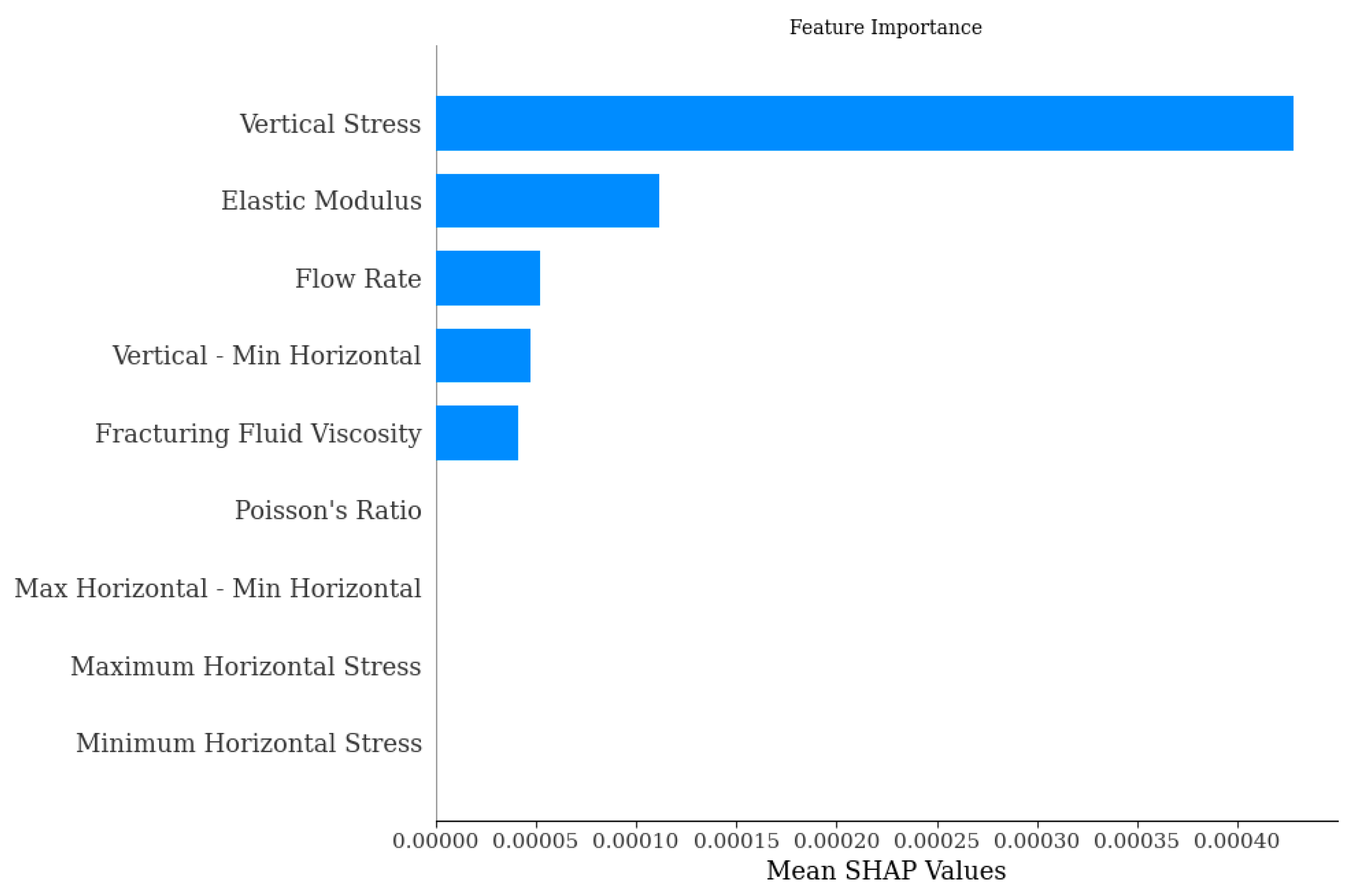
As can be seen in Figure 11, the Vertical Stresses have the greatest impact on the predicted results. Therefore, the effect of Vertical Stress on the prediction of “natural crack/main crack area ratio” is analysed separately.

Next, we analyse ‘Vertical Stress’. Looking at Figure 12, we can see that the larger SHAP values of this factor are mostly distributed in the negative direction. This result indicates that the influence factor is more likely to be negative in this scenario.

The critical value of ‘Vertical Stress’ is analysed in Figure 13. It can be seen from the figure that the value of this influence factor changes significantly at 70. That is, when the value is greater than 70, it has a negative impact in this scenario, and when it is less than 70, it has a positive impact.

(5)

Scenario 5: The Main Crack Widths

The analysis of Figure 14 shows that Vertical Stress and modulus of elasticity have a greater influence on the width of the main crack, and these two characteristics are analysed separately.

Looking at Figure 15, we can conclude that the SHAP values with larger values of this influence factor are mostly distributed in the positive direction. This phenomenon indicates that the influence of this factor is more likely to be positive in the predicting of main crack widths. For ‘Elastic Modulus’, the pattern is opposite to that of ‘Vertical Stress’.

As shown in Figure 16 and Figure 17, the SHAP value changes significantly at a value of 70 for ‘Vertical Stress’ and 25 for ‘Elastic Modulus’. This phenomenon indicates that the critical points of ‘Vertical Stress’ and ‘Elastic Modulus’ are 70 and 25, respectively.

(6)

Scenario 6: The Length of Main Cracks

The analysis of Figure 18 shows that the Vertical Stresses have the greatest influence on the predicted results and far outweigh the other features. Therefore, the Vertical Stresses are analysed separately.

Next, we analyse ‘Vertical Stress’. Looking at Figure 19, we can see that the SHAP values of this factor are mostly distributed in the positive direction. This phenomenon suggests that the influence factor is more likely to be positive in this scenario. However, there are also cases where the factor has a small value when the SHAP is positive, and similarly when the SHAP is negative. This result suggests that there is a threshold value that shifts the positive and negative influence of the factor.

As shown in Figure 20, the SHAP value changes significantly at ‘Vertical Stress’ 70. When the value is greater than 70, the influence factor has a negative influence, and when the characteristic value is less than 70, it has a positive influence.

(7)

Scenario 7: The Height of Main Crack

The analysis of Figure 21 shows that the “Vertical—Min Horizontal” has the greatest impact on the prediction results and far outweighs the other features. Therefore, “Vertical—Min Horizontal” is analysed separately.

Next, we analyse ‘Vertical—Min Horizontal’. Looking at Figure 22, we can see that the larger SHAP values of this influence factor are mostly distributed in the positive direction. This phenomenon indicates that the influence factor is more likely to be positive in this scenario.

The influence of ‘Vertical—Min Horizontal’ on this scenario is further analysed. As shown in Figure 23, the positive and negative influences shift when the value of this influence is 5.

4. Conclusions

In this paper, we propose an interpretable combinatorial machine learning-based shale compressibility evaluation method to address the problems in the traditional methods for shale compressibility evaluation, namely the limitation of the linear analyses of key influencing factors in the evaluation model and the challenge of the lack of interpretability of the data-driven model. The method combines the XGBoost machine learning model and the Bayesian optimization algorithm and introduces the SHAP value analyses for the quantitative evaluation of influencing factors. We have come to the following conclusions:

(1)

The combinatorial model effectively mined the nonlinear relationship between the influencing factors and the shale compressibility index and achieved a more accurate compressibility evaluation. Lower error rates were achieved in several scenarios, with the highest MAPE not exceeding 20%.

(2)

Our proposed method of influencing factor analyses based on SHAP value allows an in-depth analysis of the role of each influencing factor in the evaluation of fracturability. We found that ‘Vertical—Min Horizontal’ and ‘Vertical Stress’ are the most important factors. These two factors have a great influence on the fracturability of shale gas.

This work still has some shortcomings, and our proposed method is difficult to effectively accomplish the task of fracturability evaluation when sample data are sparse. In the future, it is necessary to consider how to effectively tap the nonlinear relationship between fracturability and the influencing factors in such extreme cases.

References

1. Zhou, S.; Huang, L.; Wang, G.; Wang, W.; Zhao, R.; Sun, X.; Wang, D. A review of the development in shale oil and gas wastewater desalination. Sci. Total Environ. 2023, 873, 162376. [Google Scholar] [CrossRef] [PubMed]
2. Liang, H.; You, K.; Qi, Z.; Li, H.; Yuan, Y.; Liu, S.; Zhang, L. A novel EUR prediction model for fractured horizontal shale gas wells based on material balance theory. Nat. Gas Ind. B 2024, 11, 569–580. [Google Scholar] [CrossRef]
3. Wu, J.; Zhang, S.; Cao, H.; Zheng, M.; Sun, P.; Luo, X. Fracability evaluation of shale gas reservoir—A case study in the Lower Cambrian Niutitang formation, northwestern Hunan, China. J. Petrol. Sci. Eng. 2018, 164, 675–684. [Google Scholar] [CrossRef]
4. Zeng, F.; Guo, J.; Ma, S.; Chen, Z. 3D observations of the hydraulic fracturing process for a model non-cemented horizontal well under true triaxial conditions using an X-ray CT imaging technique. J. Nat. Gas. Sci. Eng. 2018, 52, 128–140. [Google Scholar] [CrossRef]
5. Zeng, F.; Gong, G.; Zhang, Y.; Guo, J.; Jiang, J.; Hu, D.; Chen, Z. Fracability evaluation of shale reservoirs considering rock brittleness, fracture toughness, and hydraulic fracturing-induced effects. Geoenergy Sci. Eng. 2023, 229, 212069. [Google Scholar] [CrossRef]
6. Huo, Z.; Zhang, J.; Li, P.; Tang, X.; Yang, X.; Qiu, Q.; Dong, Z.; Li, Z. An improved evaluation method for the brittleness index of shale and its application—A case study from the southern north China basin. J. Nat. Gas. Sci. Eng. 2018, 59, 47–55. [Google Scholar] [CrossRef]
7. Perez, R.; Marfurt, K. Brittleness estimation from seismic measurements in unconventional reservoirs: Application to the barnett shale. In Proceedings of the SEG International Exposition and Annual Meeting, Houstonm, TX, USA, 22–27 September 2013; p. SEG-2013-0006. [Google Scholar]
8. Enderlin, M.; Alsleben, H.; Beyer, J.A. Predicting fracability in shale reservoirs. In Proceedings of the AAPG Annual Convention and Exhibition, Houston, TX, USA, 10–13 April 2011; pp. 10–13. [Google Scholar]
9. Tang, Y.; Xing, Y.; Li, L.Z.; Zhang, B.H.; Jiang, S.X. Influence factors and evaluation methods of the gas shale fracability. Earth Sci. Front. 2012, 19, 356–363. [Google Scholar]
10. Wang, D.; Ge, H.; Wang, X.; Wang, J.; Meng, F.; Suo, Y.; Han, P. A novel experimental approach for fracability evaluation in tight-gas reservoirs. J. Nat. Gas. Sci. Eng. 2015, 23, 239–249. [Google Scholar] [CrossRef]
11. Li, L.; Rong, S.; Wang, R.; Yu, S. Recent advances in artificial intelligence and machine learning for nonlinear relationship analysis and process control in drinking water treatment: A review. Chem. Eng. J. 2021, 405, 126673. [Google Scholar] [CrossRef]
12. Akinola, I.T.; Sun, Y.; Adebayo, I.G.; Wang, Z. Daily peak demand forecasting using Pelican Algorithm optimised Support Vector Machine (POA-SVM). Energy Rep. 2024, 12, 4438–4448. [Google Scholar] [CrossRef]
13. Nagar, S.; Farahbakhsh, E.; Awange, J.; Chandra, R. Remote sensing framework for geological mapping via stacked autoencoders and clustering. arXiv 2024, arXiv:2404.02180. [Google Scholar] [CrossRef]
14. Su, Q.; Chen, L.; Qian, L. Optimization of Big Data Analysis Resources Supported by XGBoost Algorithm: Comprehensive Analysis of Industry 5.0 and ESG Performance. Meas. Sens. 2024, 36, 101310. [Google Scholar] [CrossRef]
15. Hui, G.; Chen, S.; He, Y.; Wang, H.; Gu, F. Machine learning-based production forecast for shale gas in unconventional reservoirs via integration of geological and operational factors. J. Nat. Gas. Sci. Eng. 2021, 94, 104045. [Google Scholar] [CrossRef]
16. Oliveira, R.; Ott, L.; Ramos, F. Bayesian optimisation under uncertain inputs. In Proceedings of the 22nd International Conference on Artificial Intelligence and Statistics, PMLR 2019, Naha, Japan, 16–18 April 2019; pp. 1177–1184. [Google Scholar]
17. Marchant, R.; Ramos, F. Bayesian optimisation for intelligent environmental monitoring. In Proceedings of the 2012 IEEE/RSJ International Conference on Intelligent Robots and Systems, Algarve, Portugal, 7–12 October 2012; pp. 2242–2249. [Google Scholar]
18. Ru, B.; Osborne, M.A.; McLeod, M.; Granziol, D. Fast information-theoretic Bayesian optimisation. In Proceedings of the International Conference on Machine Learning, PMLR 2018, Stockholm, Sweden, 10–15 July 2018; pp. 4384–4392. [Google Scholar]
19. Abdolshah, M.; Shilton, A.; Rana, S.; Gupta, S.; Venkatesh, S. Multi-objective Bayesian optimisation with preferences over objectives. Adv. Neural Inf. Process. Syst. 2019, 32, 1–16. [Google Scholar]
20. Zhang, Y.; Pan, S. XGBoost-based prediction of electrical properties for anode aluminium foil. Mater. Today Commun. 2024, 41, 110400. [Google Scholar] [CrossRef]
21. Lewis, R.J. An Introduction to Classification and Regression Tree (CART) Analysis. In Proceedings of the Annual Meeting of the Society for Academic Emergency Medicine, San Francisco, CA, USA, 22–25 May 2000. [Google Scholar]
22. Chipman, H.A.; George, E.I.; McCulloch, R.E. Bayesian CART model search. J. Am. Stat. Assoc. 1998, 93, 935–948. [Google Scholar] [CrossRef]
23. Garrido-Merchán, E.C.; Fernández-Sánchez, D.; Hernández-Lobato, D. Parallel predictive entropy search for multi-objective Bayesian optimization with constraints applied to the tuning of machine learning algorithms. Expert. Syst. Appl. 2023, 215, 119328. [Google Scholar] [CrossRef]
24. Wen, H.; Liu, B.; Di, M.; Li, J.; Zhou, X. A SHAP-enhanced XGBoost model for interpretable prediction of coseismic landslides. Adv. Space Res. 2024, 74, 3826–3854. [Google Scholar] [CrossRef]
25. Zhang, Y. A Better Autoencoder for Image: Convolutional Autoencoder. In Proceedings of the ICONIP17-DCEC, Guangzhou, China, 14–18 October 2017; Available online: https://www.semanticscholar.org/paper/A-Better-Autoencoder-for-Image%3A-Convolutional-Zhang/b1786e74e233ac21f503f59d03f6af19a3699024 (accessed on 23 March 2017).
26. Ng, A. Sparse autoencoder. Cs294a Lect. Notes 2011, 72, 1–19. [Google Scholar]
27. Patle, A.; Chouhan, D.S. SVM kernel functions for classification. In Proceedings of the 2013 International Conference on Advances in Technology and Engineering (ICATE), Mumbai, India, 23–25 January 2013; pp. 1–9. [Google Scholar]
28. Soman, K.P.; Loganathan, R.; Ajay, V. Machine Learning with SVM and Other Kernel Methods; PHI Learning Pvt. Ltd.: Delhi, India, 2009. [Google Scholar]
Figure 1. Feature importance ranking chart for Scenario 1.
Energies 18 00186 g001
Figure 2. Summary diagram of scenario 1.
Energies 18 00186 g002
Figure 3. Vertical—Min Horizontal dependence diagram for scenario 1.
Energies 18 00186 g003
Figure 4. Feature importance ranking chart for scenario 2.
Energies 18 00186 g004
Figure 5. Summary diagram of scenario 2.
Energies 18 00186 g005
Figure 6. Vertical—Min Horizontal dependence diagram for scenario 2.
Energies 18 00186 g006
Figure 7. Feature importance ranking chart for scenario 3.
Energies 18 00186 g007
Figure 8. Summary diagram of scenario 3.
Energies 18 00186 g008
Figure 9. Vertical—Min Horizontal dependence diagram for scenario 3.
Energies 18 00186 g009
Figure 10. Vertical Stress dependence diagram for scenario 3.
Energies 18 00186 g010
Figure 11. Feature importance ranking chart for scenario 4.
Energies 18 00186 g011
Figure 12. Summary diagram of scenario 4.
Energies 18 00186 g012
Figure 13. Vertical Stress dependence diagram for scenario 4.
Energies 18 00186 g013
Figure 14. Feature importance ranking chart for scenario 5.
Energies 18 00186 g014
Figure 15. Summary diagram of scenario 5.
Energies 18 00186 g015
Figure 16. Vertical Stress dependence diagram for scenario 5.
Energies 18 00186 g016
Figure 17. Dependence diagram for the ‘Modulus of elasticity’ indicator in scenario 5.
Energies 18 00186 g017
Figure 18. Feature importance ranking chart for scenario 6.
Energies 18 00186 g018
Figure 19. Summary diagram of scenario 6.
Energies 18 00186 g019
Figure 20. Vertical Stress dependence diagram for scenario 6.
Energies 18 00186 g020
Figure 21. Feature importance ranking chart for scenario 7.
Energies 18 00186 g021
Figure 22. Summary diagram of scenario 7.
Energies 18 00186 g022
Figure 23. Vertical—Min Horizontal dependence diagram for scenario 7.
Energies 18 00186 g023