Article

A Model-Free Deep Reinforcement Learning-Based Approach for Assessment of Real-Time PV Hosting Capacity

1
Australian Power Quality Research Centre, University of Wollongong, Wollongong 2522, Australia
2
DIgSILENT Pacific, Sydney 2000, Australia
*
Author to whom correspondence should be addressed.
Energies 2024, 17(9), 2075; https://doi.org/10.3390/en17092075
Submission received: 29 March 2024 / Revised: 21 April 2024 / Accepted: 25 April 2024 / Published: 26 April 2024

Abstract

:
Assessments of the hosting capacity of electricity distribution networks are of paramount importance, as they facilitate the seamless integration of rooftop photovoltaic systems into the grid, accelerating the transition towards a more carbon neutral and sustainable system. This paper employs a deep reinforcement learning-based approach to evaluate the real-time hosting capacity of low voltage distribution networks in a model-free manner. The proposed approach only requires real-time customer voltage data and solar irradiation data to provide a fast and accurate estimate of real-time hosting capacity at each customer connection point. This study addresses the imperative for accurate electrical models, which are frequently unavailable, in evaluating the hosting capacity of electricity distribution networks. To meet this challenge, the proposed approach utilizes a deep neural network-based, data-driven model of a low-voltage electricity distribution network. This proposed methodology incorporates model-free elements, enhancing its adaptability and robustness. In addition, a comparative analysis between model-based and model-free hosting capacity assessment methods is presented, highlighting their respective strengths and weaknesses. The utilization of the proposed hosting capacity estimation model enables distribution network service providers to make well-informed decisions regarding grid planning, leading to cost minimization.

1. Introduction

Rapid integration of rooftop photovoltaic (PV) systems into low-voltage (LV) electricity distribution networks has raised concerns among distribution network service providers (DNSPs) due to its impact on power quality and reliability. High levels of PV penetration without proper consideration of integration planning may lead to adversities such as over-voltage, unnecessary curtailments, high imbalance, and thermal overloading of network elements.
The hosting capacity (HC) of an electricity distribution network may be defined as the maximum distributed generation that can be safely and reliably integrated without causing any adverse impacts to the grid. Undertaking a HC assessment allows DNSPs to plan investments more efficiently and integrate more distributed energy resources (DERs) into the grid, ensuring a cost-effective grid expansion. Traditional HC assessment strategies are commonly classified into three groups: deterministic methods, stochastic methods, and quasi-static time-series (QSTS) methods [1,2]. Deterministic methods require lower computational complexity and provide a fast estimate of HC with less accuracy [3]. Stochastic methods utilize probabilistic power flow to model uncertainties in the LV distribution network and quantify the HC [4]. QSTS methods utilize a series of steady-state power flows to accurately analyze the HC of distribution networks [5]. In contrast to other methods, QSTS simulations offer a partial representation of the system dynamics associated with control elements, providing a more refined estimate of the HC of the distribution network under study. Most of the traditional HC assessment strategies that employ QSTS simulations define the HC of a distribution system as a static value. However, the HC of a distribution network is dynamic in nature and necessitates a real-time assessment with the consideration of the temporal characteristics of the grid.
The performance index that frequently restricts the HC of LV distribution networks is the operational constraint for voltage [6]. When using the QSTS simulation-based approach, a detailed electrical model of the LV network is required to perform the necessary voltage calculations to quantify the HC with voltage as an operational constraint. However, such detailed electrical models of LV networks are not readily available for the DNSPs and, due to the sheer number of LV networks, the development of accurate LV network models entails significant time and monetary investments. This dilemma calls for the exploration of electrical model-free calculations of voltage levels. As an example, the deep neural network (DNN)-based voltage calculation using smart meter data proposed in [7] offers a pioneering and promising resolution.
In contrast to traditional HC assessment methods that calculate a static HC value, deep learning methods for HC assessments are capable of quantifying the real-time HC of LV networks and have garnered significant attention among researchers in recent years. In [8], long short-term memory (LSTM) neural networks were utilized to evaluate the real-time HC of distribution networks by identifying a mapping rule between power flow data and HC data. However, despite being a very powerful strategy for real-time HC quantification, this method requires an electrical model of the distribution network, which may not be readily available for most LV distribution systems. Deep reinforcement learning (DRL) is a subdivision of artificial intelligence (AI) and machine learning that combines the merits of reinforcement learning principles with deep learning techniques. Amidst numerous DRL algorithms, actor–critic frameworks such as deep deterministic policy gradient [9] and soft actor–critic (SAC) [10,11] are the most commonly used DRL algorithms in power systems applications since they deliver efficient performance in continuous action spaces [12]. DRL-based model-free voltage control schemes were proposed in [13,14] and a DNN-based model is used for voltage calculations; however, a DRL-based HC assessment is not presented in these studies. Model-free DRL algorithms such as SAC offer a powerful framework to solve the HC quantification problem in LV distribution networks and remain relatively unscrutinized in recent research works.
This paper proposes a model-free DRL-based approach for quantification of real-time HC of LV distribution networks. The methodology is demonstrated using an accurate electrical model of a real-world LV network and historical smart meter data. The key contributions of this paper are summarized as follows:
  • Development of a DNN-based surrogate model to perform voltage calculations using smart meter data, integrating the model-free aspects in the proposed methodology.
  • Evaluation of the real-time HC using the SAC algorithm. The proposed approach only requires real-time customer voltages and solar irradiation data to provide a fast and accurate estimate of real-time HC at each customer connection point.
  • A comparative analysis is presented between the model-based and model-free HC assessments, highlighting advantages and disadvantages of both approaches.

2. Problem Formulation

2.1. System Model and Constraints

Voltage calculations at customer connection points (CCPs) using power flow or equivalent methods are at the heart of most well-recognized HC assessment strategies. Determining the likely voltages to occur at the CCPs can assist in electricity distribution network planning such as identifying the feasibility of new connection requests, management of DERs and evaluating the impact of grid augmentations. The conventional method for voltage calculations in electricity distribution networks is via power flow analysis, which relies on an accurate model of the network that accounts for the complex network topology. Provided that LV distribution network data are readily available, power flow calculations can be easily performed using appropriate software. The HC assessment presented in this study utilizes a QSTS simulation that accounts for the temporal variability of the electricity distribution network by considering changing load patterns and uncertain weather conditions (solar irradiation). Historical time-series data gathered from smart meters for customer load active power ( P l o a d ), customer load reactive power ( Q l o a d ), and voltage at CCP ( V C C P ) are utilized in the proposed HC assessment. The voltage constraints considered are based on the AS/NZS 4777.2:2020 standard [15] which states that the active power export must cease if the local voltage exceeds 258 V.

2.2. Surrogate Model of the Network

Due to the presence of a vast number of LV networks, the topological and electrical component data of every LV distribution network is not always readily available to DNSPs. The absence of an accurate LV network model presents a significant challenge when undertaking HC assessment. However, the widespread deployment of smart meters presents an interesting opportunity to utilize P l o a d , Q l o a d , and V C C P measurements at the customer level to develop equivalent LV feeder models. The study presented in this paper utilizes a DNN-based surrogate model to approximate voltages at the CCPs. The proposed method for voltage estimation is a model-free approach that only relies on historical smart meter data and does not require an electrical model that represents the intricate details of the distribution network. A graphical illustration of the proposed DNN-based surrogate model of the LV distribution network is given in Figure 1.
The surrogate model is a nonlinear regression method that maps the active power exports ( P g e n , i ), active power load ( P l o a d , i ), and reactive power load ( Q l o a d , i ) of N number of customers to their respective voltage at the CCP ( V C C P , i ) where, i = 1,2 , 3 , , N . The input layer of the DNN requires three inputs { P g e n   , P l o a d   , Q l o a d } for each N number of customers, resulting in 3 N total number of inputs. The output layer of the DNN provides N number of outputs for the voltage V C C P of each customer. The relationship between the inputs x l , k and the output O l of a single neurone l is given in (1).
O l = F l k = 1 n ( w l , k · x l , k ) + b
where k represents the inputs from other neurones, w l , k are the corresponding weights for each input, F l is the activation function, and b is the bias term. The activation function introduces nonlinearities to the DNN and ensures that the neurone response is bounded, determining the threshold at which a neurone activates. For this study, a rectified linear unit R e L U activation function with a range of [0, 1] is used for all the hidden layers. The bias term is a learnable parameter that allows neurones to have individual response characteristics offsetting the neurone output. The relationship between DNN input { P g e n   , P l o a d   , Q l o a d } and each output V C C P , i is described in (2).
V C C P , i = k = 1 n [ w i , k   · Z i , k ( P g e n   , P l o a d   , Q l o a d ) ] + b
where Z i , k ( P g e n   , P l o a d   , Q l o a d ) is the hierarchical transformation of the input data through multiple hidden layer nonlinear mappings. The surrogate model is trained in a supervised manner and the network parameters θ (i.e., weights and biases) are updated using stochastic gradient descent by minimizing the loss function L θ . During each epoch, the loss is calculated according to mean square error as given in (3) using a sampled batch B from the training data.
L θ = 1 B n = 1 B V n V ^ n ( P g e n , n   , P l o a d , n   , Q l o a d , n ) 2
where V n is an instance of CCP voltages ( V C C P , i ) and V ^ n ( P g e n , n   , P l o a d , n   , Q l o a d , n ) is the voltage estimated by the surrogate model. The old network parameters θ o l d are updated to θ n e w by applying stochastic gradient descent as given in (4).
θ n e w = θ o l d α · L θ o l d
where α is the hyperparameter for the learning rate that regulates the rate at which the network parameters are updated. For this study, the learning rate of 0.001 is used.

3. Hosting Capacity Assessment Framework

The real-time HC of electricity distribution networks is directly impacted by the instantaneous voltage observed at CCPs and the solar irradiation levels that govern the current active power exports of DERs. The proposed HC assessment framework utilizes the SAC deep reinforcement learning algorithm to approximate the real-time HC based on the real-time observations of voltage levels at CCPs and solar irradiation levels. The exceptional performance of the SAC algorithm has garnered significant attention among researchers and emerged as a favored option for tackling complex tasks that require continuous actions in deep reinforcement learning. SAC leverages the Markov decision process (MDP) to formalize sequential decision making in reinforcement learning tasks. The following sections describe the formulation of the MDP and the application of the SAC algorithm to estimate the real-time HC.

3.1. Formulation of Markov Decision Process

In this study, the assessment of HC is formulated as a MDP with infinite time steps. MDP is a powerful mathematical framework designed to formalize the sequential decision-making process of a decision maker, otherwise known as an agent, in an uncertain environment while adhering to the Markov property. The key components of a MDP can be described as a 5-tuple { S ,   A , P ,   R ,   γ } , where: S is the state space s S , which is a comprehensive set encompassing all feasible conditions (states) of an environment accessible to the decision maker; A is the action space a A that defines the entirety of permissible decisions (actions) that an agent can take in the environment; P   : S × A × S R + represents the transition probability function that determines the conditional probability of transitioning to a new state considering the current state and action; R   :   S × A × S R represents the reward function that evaluates the agent’s performance with a numerical reward based on the action executed in a particular state; and the variable γ represents the discount factor γ 0 ,   1 .
At each time step t = { 0,1 , , T } , given the state of the environment s t , the agent takes an action a t by interacting with the environment and receiving an immediate reward r t . Consequently, the environment is then transitioned into its next state s t + 1 . The policy function π governs the sequential decision-making process of an agent, dictating the agent behaviour in the environment. Given a particular state s S , a stochastic policy presents a probability distribution π a s , including all feasible actions a A the agent can undertake. The goal of an agent in reinforcement learning is to maximize its discounted cumulative reward R s t , a t = r t + γ r t + 1 + + γ T t r T by optimizing the policy π . In reinforcement learning, the action value function Q π s , a is utilized to evaluate the policy π amidst uncertain environment transition dynamics and undertake improvements to achieve an optimal policy. According to the Markov property and leveraging the Bellman theorem, the action value function is derived in (5).
Q π s , a = E s ~ P · | s , a r s , a , s + γ   E a ~ π · | s Q π s , a
where s is the next state and a is the next action.
The formulation of the HC quantification problem as a MDP is detailed as follows.
  • Environment: the environment that the agent interacts with is the actual LV distribution network.
  • Agent: the agent is the controller that estimates the rated capacity ( S P V , i ) of the customer PV inverters.
  • State: the state of the environment at time t consists of two observations ( V C C P , i   ,   G H I i ) , where G H I i is the global horizontal irradiation at customer i .
  • Action: the action that an agent takes is the estimated real-time HC of each customer i , denoted by the rated capacity ( S P V , i ) . To reduce the search space and prevent the ( S P V , i ) estimates of the SAC algorithm reaching unrealistically high values during periods of low solar irradiation, action is clipped between 0 and M a x H C , a   c l i p S P V , i ,   0 ,   M a x H C , where M a x H C is the upper limit for PV capacity that is unlikely to be achieved during periods of high solar irradiation.
  • Reward Function: the immediate reward r t that an agent receives for taking an action a t at state s t while satisfying voltage constraints is given in (6).
    r t = ( M a x H C × N ) i = 1 N S P V , i
If voltage constraints are violated at any CCP, the reward ( r t ) is assigned the penalty value, which is a significantly high negative integer. The Markov property stipulates that the future states and actions are determined exclusively by the current state and action, rendering historical states and actions of an agent irrelevant for predicting future outcomes. As a result, the modeling process becomes more streamlined and enables the use of the SAC algorithm for determining optimal policies that maximize expected rewards.

3.2. Soft Actor–Critic Algorithm

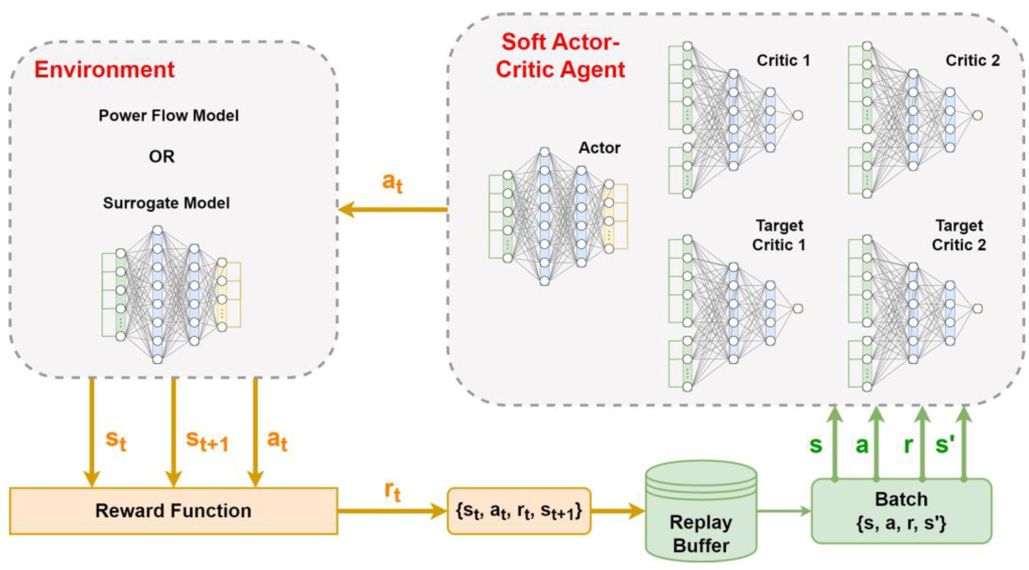
Soft actor–critic is an off-policy algorithm that optimizes a stochastic policy utilizing an actor–critic framework. The actor represents the stochastic policy π · | s , which is a probability distribution over actions for a given state. The critic represents the action value function Q π s , a that provides an estimate of the expected cumulative reward. An off-policy algorithm updates its current policy from experience samples generated by a different policy, which leads to fewer interactions with the environment and an improved sample efficiency. Through the years, SAC has undergone several iterations and enhancements [10,11]. However, for this study the SAC algorithm follows the architecture presented in [10], which utilizes a total of five feed-forward neural networks that include one actor network ( π ϕ ), two critic networks ( Q θ 1 and Q θ 2 ) , and two target critic networks ( Q θ 1 and Q θ 2 ) . The proposed framework for HC assessment using a SAC agent is illustrated in Figure 2.
The key feature of the SAC algorithm is entropy regularization, which is designed to encourage exploration and regulate the exploitation–exploration trade-off during the learning process. The entropy H π · | s of an agent’s policy represents the randomness of the agent’s actions as given in (7). A high entropy implies a more exploratory policy with less exploitation, while a low entropy implies a more deterministic policy with less exploration. The Bellman equation for entropy regularized action value function Q π s , a for the SAC algorithm is given in (8).
H π · | s = E a ~ π · | s log π · | s
Q π s , a = E s ~ P a ~ π r s , a , s + γ   Q π s , a α log π a | s
SAC employs two critic functions ( Q θ 1 , Q θ 2 ) and uses the minimum of the two critics for the policy updates; this reduces the overestimation bias and improves the learning stability. The target networks ( Q θ 1 , Q θ 2 ) of SAC facilitate the generation of more stable and reliable value estimates during the learning process. The training process of the SAC algorithm is summarized in Algorithm 1, which further elaborates the process of network parameter updates. It should be noted that the reparameterization trick is not used in the proposed SAC algorithm to reduce further additions of complexity to the HC quantification problem since the current algorithm already displays excellent performance. For the HC assessment, the learning rates used for the actor and the critic networks were 0.001 and 0.002 respectively. Five hidden layers were used for all actor and critic networks consisting of [256, 512, 1024, 512, 256] nodes. A fixed entropy coefficient of α = 0.2 and a batch size of 750 samples were used in the final SAC design, which were optimized by undertaking a sensitivity analysis.
Algorithm 1: Soft Actor–Critic
1:Initialize critics Q θ 1 , Q θ 2 and actor π ϕ with random parameters θ 1 , θ 2 , and ϕ respectively.
2:Initialize target critics Q θ 1 and Q θ 2 with main network parameters θ 1 θ 1 and θ 2 θ 2
3:Initialize the empty replay buffer D , b a t c h _ s i z e = s i z e B
4:for  t = 1  to  T  do:
5:  Observe state s of the environment and take action a ~ π · | s
6:  Execute action a . Then observe next state s and attain reward r
7:  Register experience tuple { s ,     a ,     r ,     s } in the replay buffer D
8:  if n u m b e r _ o f _ t r a n s i t i o n s _ i n _   D b a t c h _ s i z e
9:    Randomly sample a batch of B transitions { s ,   a ,   r ,   s } from D
10:    Sample next action a ~ from the actor network a ~   ~   π ϕ · | s
11:    Compute the target y r , s for the critic network updates
      y r , s = r s , a + γ min i = 1,2 Q θ i ( s , a ~ ) α log π ϕ a ~ | s
12:    Update critics Q θ 1 and Q θ 2 by gradient decent using:
   θ i 1 B s ,   a ,   r ,     s ϵ B Q θ i s , a y r , s 2      for i = 1 ,   2
13:    Update the policy ϕ by gradient accent using:
   ϕ   1 B s ϵ B min i = 1,2 Q θ i ( s , a ~ ) α log π ϕ a ~ | s ,           a ~   ~   π ϕ · | s
14:    Update target networks with ρ 1 :
   θ i ρ θ i + ( 1 ρ ) θ i         for i = 1 ,   2
15:  end if
16:end for

4. Numerical Study

4.1. Experimental Setup

A single-line diagram of the developed DIgSILENT PowerFactory LV feeder model, which consists of 28 customer connections, is given in Figure 3. The MV segment of the distribution network is represented as a Thevenin-equivalent model with a voltage source and a series impedance. The main feeders are 3-phase with a neutral conductor and the service feeders that ties the main 3-phase busbars and CCPs are single-phase with a neutral. The selected real-world LV network for the numerical study displays a significant level of phase unbalance, which is a typical feature of most LV networks. Operational constraints and the electrical characteristics of the modeled network are detailed in Table 1.
For the HC assessment, a 100% PV penetration scenario is considered, and each customer is given the opportunity to make active power exports to the network. Different data sets were used in the numerical study consisting of historical smart meter data, which are detailed in Table 2. Data Set 1 and Data Set 2 represent yearly time-series data that capture all diverse seasonal variations and are excellent for training and evaluation of the proposed DNN-based models. Data Set 3 consists of high-resolution time-series data for a single day and is ideal for the HC assessment and guarantees more accurate results.

4.2. Surrogate Model Performance Evaluation

All the proposed DNN-based models in this paper are implemented using TensorFlow 2, which provides a high-level API and simplifies the process of deploying deep learning models. The DNN-based surrogate model is trained for 3000 epochs with a batch size of 48 to capture the complex mapping relationship between the inputs ( P g e n   , P l o a d   ,   Q l o a d ) and output ( V C C P ) . As illustrated in Figure 1 and considering that there are 28 customer connections in the LV network, the input layer of the surrogate model consists of 28 × 3 = 84 nodes. The hidden layers consist of five fully connected dense layers of size [256, 512, 1024, 512, 256] and the output layer consists of 28 nodes providing V C C P of each customer. Hyperparameters of the surrogate model, i.e., hidden layer size, batch size, and learning rate, were optimized by conducting sensitivity analysis.
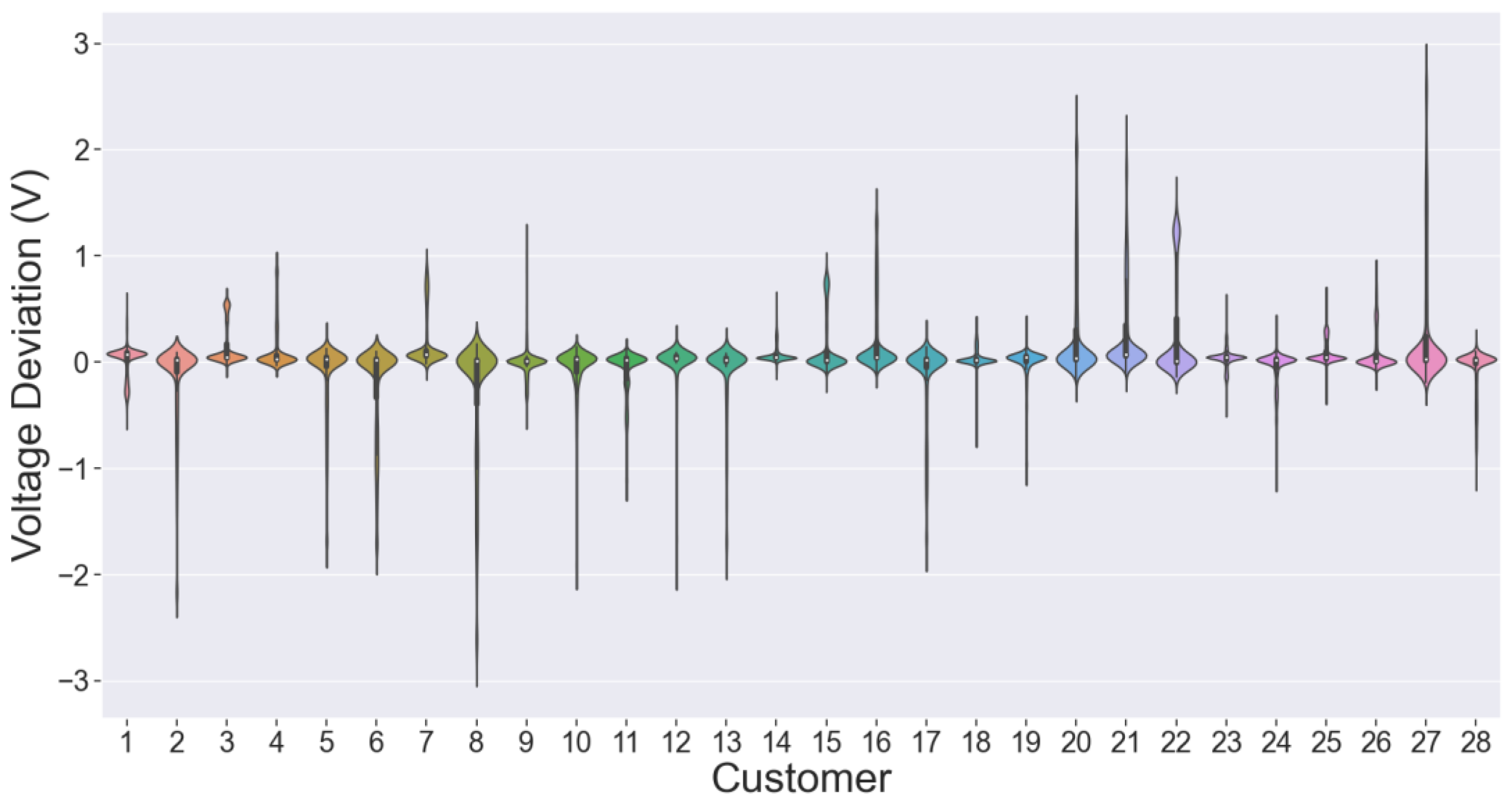
The training process of the surrogate model follows the methodology described in Section 2.2 and, upon completion of the training iterations, the performance of the trained model must be evaluated. Data Set 2 is used for the performance evaluation, which consists of completely different samples of data from that of Data Set 1, which was used for training. Voltage deviation is used as the metric to evaluate the surrogate model, which is defined as V t a r g e t ( i , t ) V C C P ( i , t ) for each customer i at time step t , where V t a r g e t is the actual smart meter voltage at CCP according to Data Set 2. The voltage deviations of the surrogate model calculated for all customers of the LV network are illustrated as violin plots in Figure 4. Based on the calculated voltage deviation results, the maximum voltage deviation is identified to be ±3 V across all the customers. Therefore, it can be concluded that the trained surrogate model is capable of delivering accurate estimates of the voltages at the CCPs.

4.3. Hosting Capacity Assessment Results

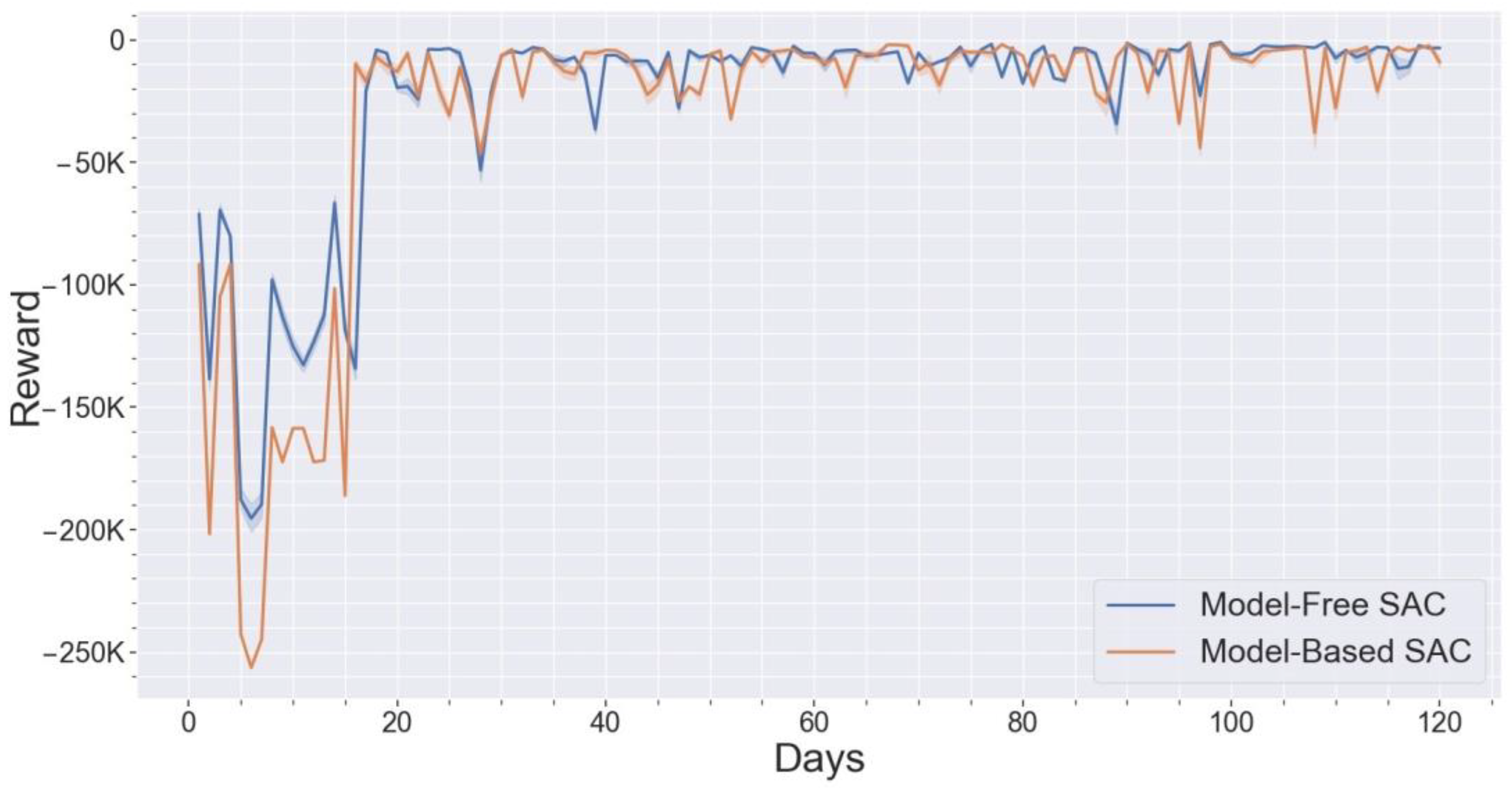
The LV network PowerFactory model and the surrogate model were used to train two distinct SAC agents (model-based SAC and model-free SAC, respectively) for the HC assessments. The design and the hyperparameters of the two agents are identical except for the environment that they interact with. Data Set 1 is used for the training of both SAC agents and for each time step, 12 episodes were considered, resulting in a total of 5760 × 12 = 69,120 training episodes. The learning curves of the model-free and model-based SAC agents are illustrated in Figure 5. Both agents converge to a similar reward and display similar learning efficiency, which is consistent with the fact that they are of similar design. Minor deviations in the two learning curves can be explained by the disparity between the PowerFactory model and the surrogate model. Upon the completion of training, the network parameters of both SAC agents were saved and utilized for the HC assessment.
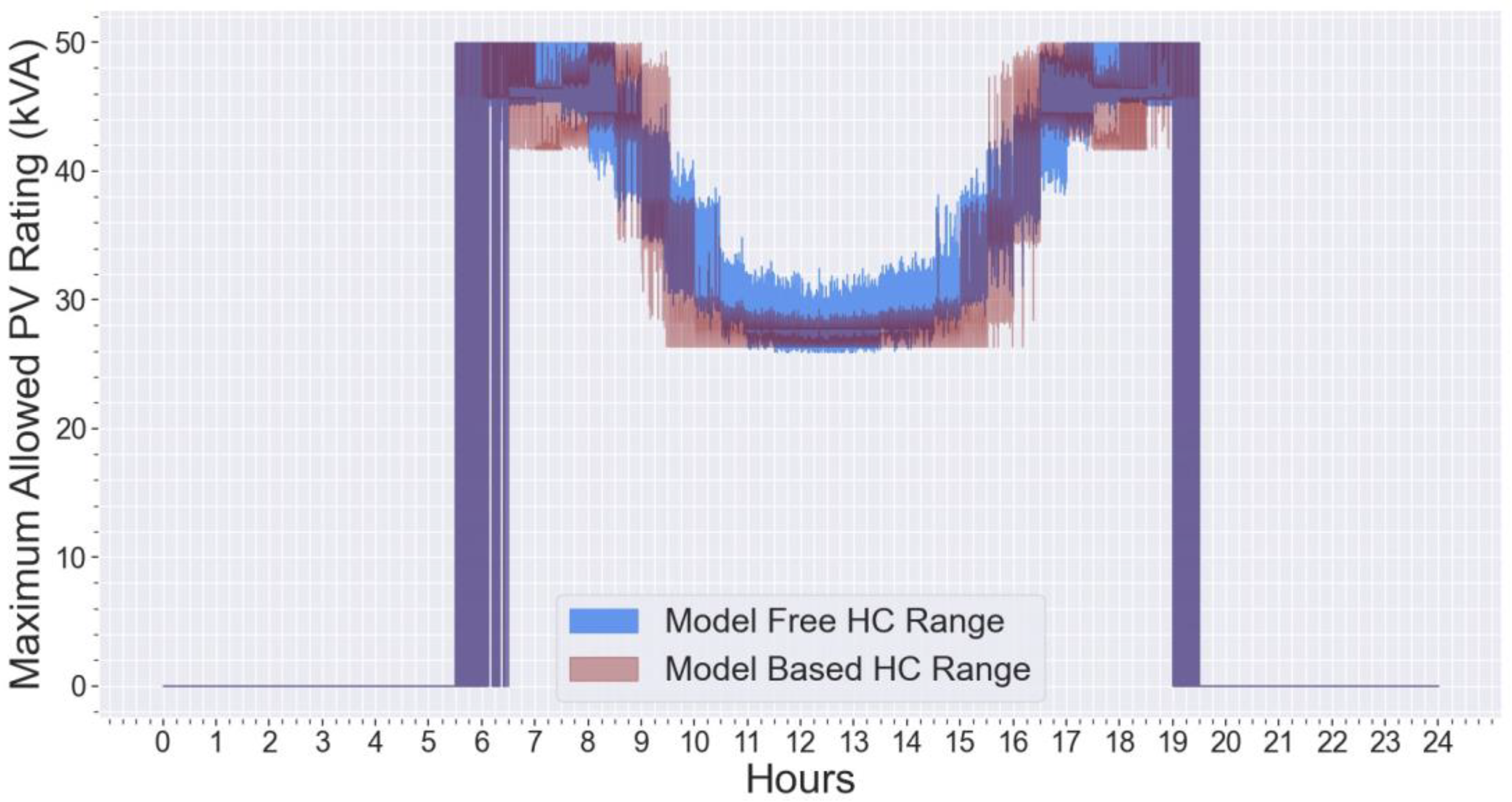
Data Set 3 was utilized to undertake two high-resolution QSTS simulations and analyze the real-time HC of the LV distribution network by each SAC agent. The trained SAC agents estimate the real-time HC for each customer within milliseconds using just customer voltage V C C P , i   from smart meter measurements and live solar irradiation G H I i data as inputs. The real-time HC of all customers estimated by the SAC agents for a duration of 24 h is illustrated in Figure 6, depicted as a shaded region. The validity of the estimated real-time HC values can be confirmed by performing a power flow calculation to check for voltage constraint violations.
It should be noted that HC is evaluated as the maximum allowed PV rating for each customer installation. In Figure 6, HC is defined only for durations when G H I is present, with HC assigned a value of zero during nighttime periods. This explains the fluctuation of HC between zero and M a x H C (where M a x H C = 50 kVA for this numerical study and is an arbitrary value, as detailed in Section 3.1) during the periods around sunrise and sunset when G H I values are close to or at zero. To ensure fairness between customers for active power exports, the HC estimates of customers by the SAC agent are clipped between ±10% of the mean hosting capacity among customers at each instance of time. This characteristic is evident in Figure 6, where the HC range across all customers does not vary by more than ±10% at any given point in time. Considering the model-based HC values as the benchmark, it is evident from the results that the model-free SAC agent slightly overestimates the real-time HC during periods of high G H I . However, overall results indicate that the quantified model-free HC values and the model-based HC values are more or less similar to each other.

5. Discussion

The proposed method for real-time HC evaluation is superior to traditional HC evaluation methods in different aspects. The dynamic and adaptive nature of the proposed real-time HC evaluation strategy enables DNSPs to make informed decisions related to grid planning and expansions while responding to grid constraints. To evaluate the real-time HC more accurately using the proposed model-free SAC algorithm with a surrogate model, the actual LV distribution network needs to exhibit some level of PV penetration at the current stage. Since the proposed DNN-based surrogate model features as a regression model, minimal PV penetration levels result in sparse training data representing active power exports and ultimately lead to suboptimal mapping of active and reactive powers to voltages. Based on the sensitivity analysis conducted using a surrogate model for HC evaluation, a minimum of roughly 30% PV penetration should exist in the current LV distribution network to yield accurate results.
Model-based high-resolution QSTS simulations generally take a significant amount of time for the simulations to complete. This is mainly due to the time taken for the power flow calculation itself and the time delay caused by the data transfer between the power flow software and the scripting software. The use of a DNN-based surrogate model bypasses this time delay and significantly reduces the simulation time of the QSTS simulations. After the training of SAC agents, any persisting exploratory actions of the SAC algorithm due to entropy regulation may result in slight errors in the quantified HC. However, this error can be negated by using SAC as a deterministic agent for the HC assessment after training by assigning the entropy coefficient to α = 0 . Overall, SAC is a powerful algorithm that is less sensitive to hyperparameters and delivers exceptional performance in high-dimensional and continuous action spaces.

6. Conclusions

An electrical model of a real-world 3-phase LV distribution network was developed and a DNN-based surrogate model of the same LV network was designed and its performance was evaluated. A model-based SAC agent and a model-free SAC agent were trained using the electrical model and the DNN-based surrogate model, respectively. In this paper, the real-time HC of the LV distribution network is evaluated using both the trained model-based SAC agent and the model-free SAC agent. Furthermore, a comparative analysis is presented between the proposed model-based and model-free HC assessments. The experimental results demonstrate the excellent performance of the proposed real-time HC quantification strategy.
The proposed methodology represents a notable advancement over traditional HC quantification methods, which typically yield static estimates. By contrast, the proposed approach utilizes trained neural networks to provide HC estimates within milliseconds, eliminating the need for lengthy calculations inherent in traditional methods. This methodology leverages artificial intelligence and machine learning to enable the application of advanced algorithms capable of more effectively addressing complex, nonlinear, and non-convex optimization challenges compared to conventional techniques.
Future work entails the extension of the presented HC quantification methodology as an advanced coordinated control strategy to regulate the dispatched active and reactive power of customer PV systems and enhance the overall HC of the grid. Further investigation will be conducted to develop a more precise surrogate model of the LV distribution network capable of adjusting to network variations without necessitating significant changes to the neural network architecture or requiring extensive retraining.

Author Contributions

Conceptualization, J.S., D.A.R. and A.R.; methodology, J.S. and A.R.; software, J.S.; validation, D.A.R. and A.R.; writing—original draft preparation, J.S.; writing—review and editing, A.R. and D.A.R. All authors have read and agreed to the published version of the manuscript.

Funding

This research received no external funding.

Data Availability Statement

Developed Python scripts, trained neural network models and the DIgSILENT PowerFactory LV network model can be downloaded at: https://github.com/suchithra-jude/A-model-free-DRL-based-approach-for-the-assessment-of-real-time-PV-hosting-capacity.git.

Acknowledgments

The authors wish to acknowledge the support of Endeavour Energy through the Australian Power Quality Research Centre in providing funding for the resources, which made this research possible.

Conflicts of Interest

Author Amin Rajabi was employed by the company DIgSILENT Pacific. The remaining authors declare that the research was conducted in the absence of any commercial or financial relationships that could be construed as a potential conflict of interest.

References

  1. Rajabi, A.; Elphick, S.; David, J.; Pors, A.; Robinson, D. Innovative approaches for assessing and enhancing the hosting capacity of PV-rich distribution networks: An Australian perspective. Renew. Sustain. Energy Rev. 2022, 161, 112365. [Google Scholar] [CrossRef]
  2. Mulenga, E.; Bollen, M.H.J.; Etherden, N. A review of hosting capacity quantification methods for photovoltaics in low-voltage distribution grids. Int. J. Electr. Power Energy Syst. 2020, 115, 105445. [Google Scholar] [CrossRef]
  3. Ebe, F.; Idlbi, B.; Morris, J.; Heilscher, G.; Meier, F. Evaluation of PV hosting capacities of distribution grids with utilisation of solar roof potential analyses. CIRED Open Access Proc. J. 2017, 2017, 2265–2269. [Google Scholar] [CrossRef]
  4. Kabir, M.N.; Mishra, Y.; Bansal, R.C. Probabilistic load flow for distribution systems with uncertain PV generation. Appl. Energy 2016, 163, 343–351. [Google Scholar] [CrossRef]
  5. Deboever, J.; Grijalva, S.; Reno, M.J.; Broderick, R.J. Fast Quasi-Static Time-Series (QSTS) for yearlong PV impact studies using vector quantization. Sol. Energy 2018, 159, 538–547. [Google Scholar] [CrossRef]
  6. Torquato, R.; Salles, D.; Pereira, C.O.; Meira, P.C.M.; Freitas, W. A Comprehensive Assessment of PV Hosting Capacity on Low-Voltage Distribution Systems. IEEE Trans. Power Deliv. 2018, 33, 1002–1012. [Google Scholar] [CrossRef]
  7. Bassi, V.; Ochoa, L.F.; Alpcan, T.; Leckie, C. Electrical Model-Free Voltage Calculations Using Neural Networks and Smart Meter Data. IEEE Trans. Smart Grid 2022, 14, 3271–3282. [Google Scholar] [CrossRef]
  8. Wu, J.T.; Yuan, J.; Weng, Y.; Ayyanar, R. Spatial-Temporal Deep Learning for Hosting Capacity Analysis in Distribution Grids. IEEE Trans. Smart Grid 2022, 14, 354–364. [Google Scholar] [CrossRef]
  9. Silver, D.; Lever, G.; Heess, N.; Degris, T.; Wierstra, D.; Riedmiller, M. Deterministic policy gradient algorithms. In Proceedings of the 31st International Conference on International Conference on Machine Learning, Beijing, China, 21–26 June 2014; Volume 1, pp. 605–619. [Google Scholar]
  10. Haarnoja, T.; Zhou, A.; Hartikainen, K.; Tucker, G.; Ha, S.; Tan, J.; Kumar, V.; Zhu, H.; Gupta, A.; Abbeel, P.; et al. Soft Actor-Critic Algorithms and Applications. arXiv 2018, arXiv:1812.05905. [Google Scholar]
  11. Haarnoja, T.; Zhou, A.; Abbeel, P.; Levine, S. Soft Actor-Critic: Off-Policy Maximum Entropy Deep Reinforcement Learning with a Stochastic Actor. arXiv 2018, arXiv:1801.01290. [Google Scholar]
  12. Chen, X.; Qu, G.; Tang, Y.; Low, S.; Li, N. Reinforcement Learning for Selective Key Applications in Power Systems: Recent Advances and Future Challenges. IEEE Trans. Smart Grid 2022, 13, 2935–2958. [Google Scholar] [CrossRef]
  13. Cao, D.; Zhao, J.; Hu, W.; Ding, F.; Yu, N.; Huang, Q.; Chen, Z. Model-free voltage control of active distribution system with PVs using surrogate model-based deep reinforcement learning. Appl. Energy 2022, 306, 117982. [Google Scholar] [CrossRef]
  14. Kou, P.; Liang, D.; Wang, C.; Wu, Z.; Gao, L. Safe deep reinforcement learning-based constrained optimal control scheme for active distribution networks. Appl. Energy 2020, 264, 114772. [Google Scholar] [CrossRef]
  15. AS/NZS 4777.2:2020; Grid Connection of Energy Systems via Inverters, Part 2: Inverter Requirements. Australian/New Zealand Standards: Sydney, Australia, 2020.
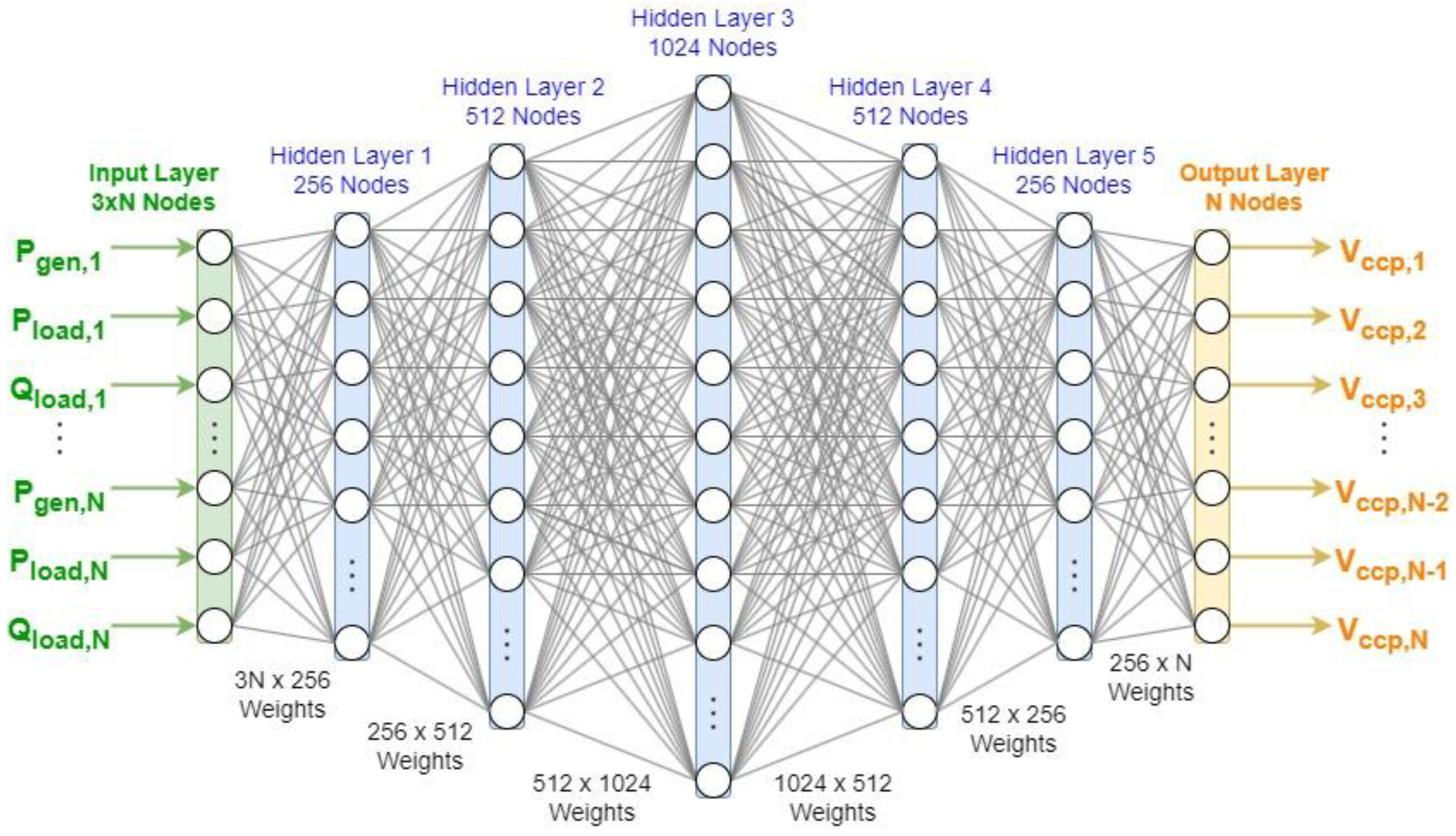
Figure 1. DNN-based surrogate model of the LV distribution network.
Energies 17 02075 g001
Figure 2. Diagrammatic representation of the proposed real-time HC assessment framework.
Energies 17 02075 g002
Figure 3. Single-line diagram of the modeled LV distribution network.
Energies 17 02075 g003
Figure 4. Voltage deviation of the LV network customer voltages evaluated by the surrogate model.
Energies 17 02075 g004
Figure 5. Learning curve of the model-free and model-based SAC agents.
Energies 17 02075 g005
Figure 6. Average real-time HC across customers in the LV distribution network.
Energies 17 02075 g006
Table 1. LV network electrical characteristics and constraints.
R1 Ohm/kmX1
Ohm/km
R0
Ohm/km
X0
Ohm/km
Main Feeder0.2985570.2596331.1325080.945961
Service Feeder1.4800030.088--
Network Constraints
Nominal voltage = 230 VMaximum voltage limit = 258 VMinimum voltage limit = 218 VTransformer rating = 1 MVA
Table 2. Data sets used in the numerical study.
Data SetDaysTime Step ResolutionTime StepsSimulation
112030 min5760Training of the surrogate model and the SAC agents
212030 min5760Surrogate model evaluation
315 s17,280HC assessment
Disclaimer/Publisher’s Note: The statements, opinions and data contained in all publications are solely those of the individual author(s) and contributor(s) and not of MDPI and/or the editor(s). MDPI and/or the editor(s) disclaim responsibility for any injury to people or property resulting from any ideas, methods, instructions or products referred to in the content.