Automatic Generation Control of a Multi-Area Hybrid Renewable Energy System Using a Proposed Novel GA-Fuzzy Logic Self-Tuning PID Controller

Abstract

Human activities overwhelm our environment with CO₂ and other global warming issues. The current electricity landscape necessitates a superior, continuous power supply and addressing such environmental concerns. These issues can be resolved by incorporating renewable energy sources (RESs) into the utility grid. Thus, this paper presents an optimized hybrid fuzzy logic self-tuning PID controller to control the automatic generation control (AGC) of various renewable sources. This controller regulates the frequency deviations of the power system and governs the change in the tie-line load of a multi-area hybrid energy system composed of wind, biomass, and photovoltaic energy sources. MATLAB Simulink software was applied to design and test the system. The PID controller has been tuned using four algorithms, namely, genetic algorithm (GA), pattern search (PS), simulated annealing (SA), and particle swarm optimization (PSO), and we compared the results with the proposed novel optimized PID controller (GA-fuzzy logic self-tuning technique) to validate it. The results show the superiority of the proposed hybrid GA-fuzzy logic self-tuning algorithm over the other algorithms in bringing the power system back to its regular operation. The paper also proposes an operation strategy to lower the utilization of biomass energy in the presence of other renewable energy sources.

1. Introduction

The main objective of the electric power control technique is to generate power and deliver it to the grid economically while preserving the voltage and frequency within their permissible limits. Fluctuation in real power commonly affects the system frequency, while reactive power impacts the voltage magnitude. Hence, real and reactive power are controlled separately. Load frequency control (LFC) technology controls real power and frequency and is the foundation of many modern concepts for controlling large systems.

When a sudden load occurs in the system, the turbine speed decreases before the governor can calibrate the input of that system to the new load. As the turbine speed decreases, the error signal becomes smaller and smaller, and the governor flyball’s position becomes closer to the constant speed point; yet, there will be an offset in the speed. An integrator is usually added to overcome the offset and restore the speed to its nominal value [1]. As the load changes perpetually, the generation is regulated automatically to restore the speed; accordingly, the frequency is set to the nominal value. This mechanism is known as the AGC. The role of AGC in power grids is to distribute the loads among the stations and the generators to attain optimal generation and to control the scheduled interchanges of tie-line power while maintaining a steady frequency. Various studies have been conducted on LFC and AGC, which address various modern control systems for the power system’s successful generation [1].

Figure 1 shows the AGC of an isolated power system, where H is the per unit inertia constant, its unit is seconds, and its value ranges between zero and one second based on the size and the type of the machine. The D is the damping coefficient. R is the droop voltage magnitude; governors typically have a 5 to 6 percent speed regulation from zero to full load. B is the frequency bias factor. $\Delta \omega \left(s\right)$ is the frequency sensitive load change. $\Delta P_L\left(s\right)$ is the non-frequency sensitive load change. $\Delta P_m$ is the change in mechanical power output. $\Delta P_V$ is the change in steam valve position. $\Delta P_{ref}$ is the reference set power. $\Delta P_g$ is the speed governor comparator, ${\tau }_g$ is a simple time constant, and ${\tau }_T$ is the time constant of the prime mover, which is in the range between 0.2 and 2.0 s.

$$B=\frac{1}{R}+D$$

(1)

$$\Delta P_V\left(s\right)=\frac{1}{1+{\tau }_g}\Delta P_g\left(s\right)$$

(2)

$$\mathrm{H}=\frac{\mathrm{Kinetic} \mathrm{energy} \mathrm{in} \mathrm{MJ} \mathrm{at} \mathrm{rated} \mathrm{speed}}{\mathrm{Machine} \mathrm{rating} \mathrm{in} \mathrm{MVA}}=\frac{W_K}{S_B}$$

(3)

$${\mathrm{G}}_{\mathrm{T}}\left(s\right)=\frac{\Delta P_m\left(s\right)}{\Delta P_V\left(s\right)}=\frac{1}{1+{\tau }_{T}s}$$

(4)

The energy sources applied in AGC and LFC studies were not limited to conventional energy sources but also included RES. Even though biomass is considered an RES, minimal research has been conducted on its application as an energy source in power plants. In the United States, until the middle of the 1800s, biomass was the primary source of the nation’s annual energy consumption. By 2022, the United States’ primary energy consumption was about five percent from biomass [2]. Figure 2a depicts the US biomass energy consumption in the year 2022, where the consumption was 2266 trillion British thermal units (TBtu)—1565 TBtu, 539 TBtu, 413 TBtu, and 147 TBtu from the industrial, transportation, residential, electric power, and commercial sector, respectively. Figure 2b depicts the energy consumed from biomass in the US, which accounts for 5% of the total energy consumption [2].

Paper [3] presents an overview of applying biomass as an RES to generate heat and power. Different technologies are introduced. Paper [4] integrated biomass energy into an IEEE 30 bus test system composed of six generating units to minimize the conventional fuel ratio and the greenhouse gases. In [5], H. H. H. Aly presented dynamic models of tidal current turbines applying a direct drive permanent magnet synchronous generator (DDPMSG) and doubly fed induction generator (DFIG). The stability analysis results found better performance of the tidal current turbines using a DDPMSG over the DFIG one and that applying PID controllers improves the stability analysis.

K. Jagatheesan et al. [6] presented a nature bio-inspired firefly (FFA)-tuned PID controller for AGC of a multi-area reheat thermal power system. The results derived were compared with GA and PSO-tuned PID controllers. From the results derived, the proposed technique gave the best results regarding the Integral of Time and Absolute Error (ITAE), settling time, undershoot, and overshoot. D. K. Gupta et al. [7] introduced a PID controller tuned using a nature bio-inspired FFA, Particle Swarm Optimization (PSO), and the Gravitational Search Algorithm (GSA) for AGC of multi-area hydro, gas, and thermal power systems. ITAE is considered as the objective function. The results derived from the proposed algorithm show the efficiency of applying it to obtain stable frequency and load responses. Rabindra R. K. Sahu, S. Panda, and S. Pradhan [8] presented a novel hybrid firefly algorithm and pattern search (HFA–PS)-tuned PID model for AGC of multi-area power systems considering the Generation Rate Constraint (GRC). ITAE has been considered to be the objective function. The results derived from the proposed model demonstrated superior outcomes compared to some modern heuristic optimization techniques such as the Bacteria Foraging Optimization Algorithm (BFOA), Genetic Algorithm (GA), and conventional Ziegler–Nichols (ZN)-based PI/PID controllers for the same interconnected power system. A. Ghosh et al. [9] proposed an optimized Ziegler–Nichols (ZN)-based tuned PID controller for AGC of a single-area thermal power system and a multi-area PV-integrated thermal power system.

A. K. Barisal and S. Mishra [10] presented a nature bio-inspired BFOA, PSO, and Improved-PSO-tuned PID controller for AGC of two-area diesel, hydro, thermal, and wind power systems. ITAE is considered as the objective function. The results derived from the proposed algorithm show its effectiveness in obtaining a stable frequency response and load response on the tie-line. Applying parallel DC/AC links enhanced the dynamic stability of the system and dropped the cost index. S. K. Bhagat et al. [11] introduced a hybrid PSO-GA controller with a tilt-integral-derivative (TIDN) filter controller for AGC control of a multi-area power system.

H. Haes Alhelou, M. E. Hamedani Golshan, and M. Hajiakbari Fini [12] introduced a wind-driven optimization (WDO)-algorithm-tuned PID controller for the three-area power system LFC. C. Huang et al. [13] presented a natural bio-inspired Gravitational Search Algorithm (GSA)-based linear active disturbance rejection control (LADRC) approach for the LFC of the two-area power system. ITAE is considered as the objective function. The results derived from the proposed algorithm show the efficiency of applying it to obtain stable frequency and load responses. H. Changmai and M. Buragohain [14] presented a natural bio-inspired, GA-tuned, PID-controller-based linear quadratic regulator (LQR) for the LFC of the two-area power system. In [15], Y. L. Karnavas and E. Nivolianiti introduced a nature bio-inspired Harris Hawks Optimization (HHO) for LFC of an isolated multi-source power system. By comparing the proposed algorithm with the Whale Optimization Algorithm (WOA), Grey Wolf Optimizer (GWO), and PSO, it was found that the proposed algorithm exhibited superior performance in terms of power stability, settling time, overshoot, and undershoot.

R. Shankar, K. Chatterjee, and R. Bhushan studied, in [16], the LFC of a multi-source two-area power system with an energy storage system (redox flow battery) in a deregulated power environment. An opposition-based harmonic search (OHS) technique has been applied to tune the PID controller. Economic load dispatch has been integrated into the LFC. The redox flow battery is applied to absorb any transient or sudden load change. In [17], E. Çelik et al. presented a nature bio-inspired dragonfly search algorithm (DSA)-tuned PID controller for LFC of a single-area and two-area thermal power system. A (1 + PD)-PID cascade controller has been optimized via DSA using ITAE to obtain optimal results. N. R. Babu et al. [18] studied the impact of different solar insulation types on the LFC of two-area thermal power systems. Tilt integral minus derivative control (TI-DN) with filter has been applied as a supplementary controller with the crow search optimization (CSO) technique to optimize LFC. The paper found that the amalgamation of HVDC with AC tie-line amalgamates system dynamics. R. R. Kumar, A. K. Yadav, and M. Ramesh [19] presented a PID-based LQR controller for the LFC of a wind/solar-based renewable microgrid. The results reveal the proposed controller’s dynamic and frequency response effectiveness.

M. Amaro Pinazo, R. Antara Arias, and J. Mirez Carrillo reviewed, in [20], the analysis and performance of four different control technologies for wind turbines based on electromagnetic and mechanical torques. Babu, N.R. et al. presented in [18] the effects of different solar insolation types on two thermal area LFC systems. They showed that integrating HVDC with an AC tie-line improved system dynamics.V. Patel, D. Guha, and S. Purwar [21] presented a fractional-order adaptive sliding mode control (FO-ASMC) to improve the frequency regulation of power systems. The efficiency of the proposed control scheme has been tested under different load and wind disruptions. The results reveal this method’s effectiveness in frequency response and system stability. P. Saxena, N. Singh, and A. K. Pandey studied, in [22], the frequency fault ride-through (FFRT) capability of solar-based microgrids and proposed an adaptive PI-based virtual damping (PIVD) controller to augment the dynamic performance. This controller de-loads solar power while tracking frequency errors; the de-load process produces virtual inertia reserve (VIR) to stabilize the grid in case of contingency, in place of batteries. The model has been validated via MATLAB, and the results derived showed that the suggested model is qualified to ride through severe fault scenarios with minimal frequency disruption.

W. Guo and J. Yang presented, in [23], a novel nonlinear mathematical model of hydro-turbine governing systems based on the nonlinear characteristics of penstock head loss. P. Dash, L. C. Saikia, and N. Sinha proposed, in [24], a Flower Pollination Algorithm (FPA)-tuned Proportional Integral-Proportional Derivative (PI-PD) cascade controller for AGC of a four-thermal power system. R. El-Sehiemy et al. presented, in [25], an Artificial Rabbits Algorithm (ARA)-optimized PID controller for LFC of multi-area power systems. ITAE has been considered to be the objective function. The results derived from the proposed model demonstrated superior outcomes compared to some modern heuristic optimization techniques such as PSO, differential evolution (DE), JAYA optimizer, and self-adaptive multi-population elitist (SAMPE) JAYA.

This work proposes and optimizes a multi-area hybrid renewable energy system composed of three renewable energy sources: wind, biomass, and solar. The proposed work is validated by using software programs that can simulate it. MATLAB R2017b software is a powerful tool that allows users to predict a system’s behavior. It can be used to evaluate a new design, diagnose problems with an existing design, and test a system under various conditions. A mathematical model of the system is needed to run a simulation, which can be expressed as a block diagram, code, schematic, or even state diagram. As Peck (2004, p. 4) puts it:

When a researcher builds a simulation model, they have created a world in which they have access to all of the laws and components of that world, and the relationships among those components. Not only do researchers have access to these things, but they can also manipulate them. To the extent that researchers can match their simulated world to the real world, they should be able to read things off the simulated world that will tell them something about the real world.

MATLAB Simulink R2017b is applied to design and optimize the subjected model. GA, PS, SA, PSO, and the novel GA-fuzzy logic self-tuning techniques are used to tune the PID controller’s parameters by minimizing ITAE and the net present cost (NPC). The novelty here is integrating biomass into AGC and developing the GA-fuzzy algorithm. System performance is examined by considering the frequency and load disturbance in all three areas. The effectiveness of the novel GA-fuzzy logic self-tuning technique was proved by comparing its performance with the other four optimization techniques. The paper also presents an operating strategy to utilize wind, solar, and biomass energy sources.

2. PID Controller and the Proposed Hybrid Energy System

This work presents the novel GA-fuzzy logic self-tuning algorithm and some heuristic-based optimization techniques for AGC of multi-area hybrid energy systems. Regarding the heuristic-based optimization techniques, four different optimization techniques, namely, GA, PS, SA, and PSO, were applied. These algorithms, in addition to the novel GA-fuzzy logic self-tuning algorithm, are applied to tune the PID controller’s parameters, diminish the fluctuation in the frequency, and control the power flow in the plants and the tie-line.

The PID controller is one of the most used controllers in many disciplines. Its output could be represented by Equation (5).

$$y\left(t\right)=K_{p}x\left(t\right)+K_i\int x\left(t\right)dt+K_d\frac{d\left(x\right)t}{dt}$$

(5)

where $x\left(t\right)$, $y\left(t\right)$, $K_p$, $K_i$, and $K_d$ correspond to the input, the output, the proportional gain, the integral gain, and the derivative gain, respectively.

The objective functions in this work are ITAE and NPC (see Equations (6) and (16)). ITAE is considered to be the objective function because it reduces the error during the initial transient response. Such a criterion is recommended when a fast response and settling time are desired. The goal is to tune the PID parameters by minimizing the objective function.

$$\mathrm{ITAE}={{\displaystyle \int }}_0^{t_s}t\times \left|x\left(t\right)\right|.dt$$

(6)

where $t_s$ is simulation time, tuning the controller’s parameters is crucial for optimal operation.

Research papers consider many performance indices, such as the integral of absolute error (IAE), integral of squared error (ISE), integral of time-weighted squared error (ITSE), and ITAE. However, ITAE was proven to give satisfactory optimization results concerning LFC and AGC regarding settling time, undershoot, and overshoot. Therefore, we consider ITAE to be an objective function in our current work.

$$\mathrm{ITAE}={{\displaystyle \int }}_0^{t_s}\left(\left|\Delta F_W\right|+\left|\Delta F_B\right|+\left|\Delta F_{PV}\right|+\left|\Delta P_{tl}\right|\right)·t·dt$$

(7)

where $\Delta F_W$, $\Delta F_B$, and $\Delta F_{PV}$ represent the variation in frequency in the wind power plant, the biomass power plant, and the photovoltaic power plant, respectively; moreover $\Delta P_{tl}$ represents the variation in tie-line power. The proposed optimization technique minimizes the objective function for finding the PID controller’s parameters.

The constraints were as follows:

$$\begin{gathered} K_{p_{min}}<K_p<K_{p_{max}}, \\ {K}_{i_{min}}<K_i<K_{i_{max}}, \\ {K}_{d_{min}}<K_d<K_{d_{max}} \end{gathered}$$

where $K_{p_{min}}$, $K_{p_{max}}$, $K_{i_{min}}$, $K_{i_{max}}$, $K_{d_{min}}$, and $K_{d_{max}}$ are the minimum proportional gain, the maximum proportional gain, the minimum integral gain, the maximum integral gain, the minimum derivative gain, and the maximum derivative gain, respectively.

From Equation (5), we have:

$$Y_1=K_{p_1}\times AC{E}_W+K_{i_1}\times \int AC{E}_W+K_{d_1}\times \frac{dAC{E}_W}{dt},$$

(8)

$$Y_2=K_{p_2}\times AC{E}_B+K_{i_2}\times \int AC{E}_B+K_{d_2}\times \frac{dAC{E}_B}{dt},$$

(9)

$$Y_3=K_{p_3}\times AC{E}_{PV}+K_{i_3}\times \int AC{E}_{PV}+K_{d_3}\times \frac{dAC{E}_{PV}}{dt}$$

(10)

where ACE is the area control error; ACE is the difference between each plant’s electric power into the grid via generation or purchases and the electric power taken out as load, losses, or sales.

$$\begin{gathered} AC{E}_W=B_1\Delta F_W+\Delta P_{tl} \\ AC{E}_B=B_2\Delta F_B+\Delta P_{tl} \\ AC{E}_{PV}=B_3\Delta F_{PV}+\Delta P_{tl} \end{gathered}$$

where $AC{E}_W, AC{E}_B$ and $AC{E}_{PV}$ are the area control errors for the wind, biomass, and solar power plants, respectively. Figure 3 and the ACE equations show that ACE relies on the frequency and the tie-line power, where ACE is the input. Appendix A shows the parameters for the proposed AGC of the model depicted in Figure 3.

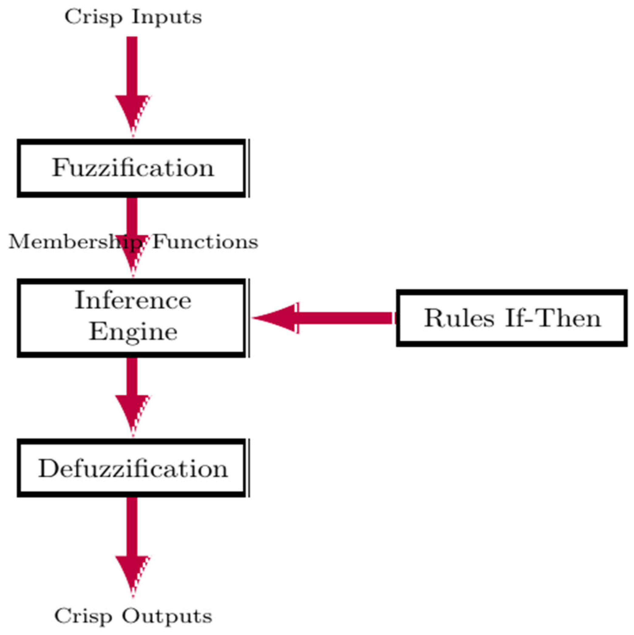
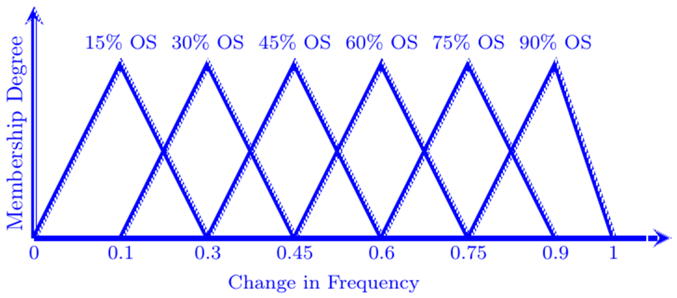
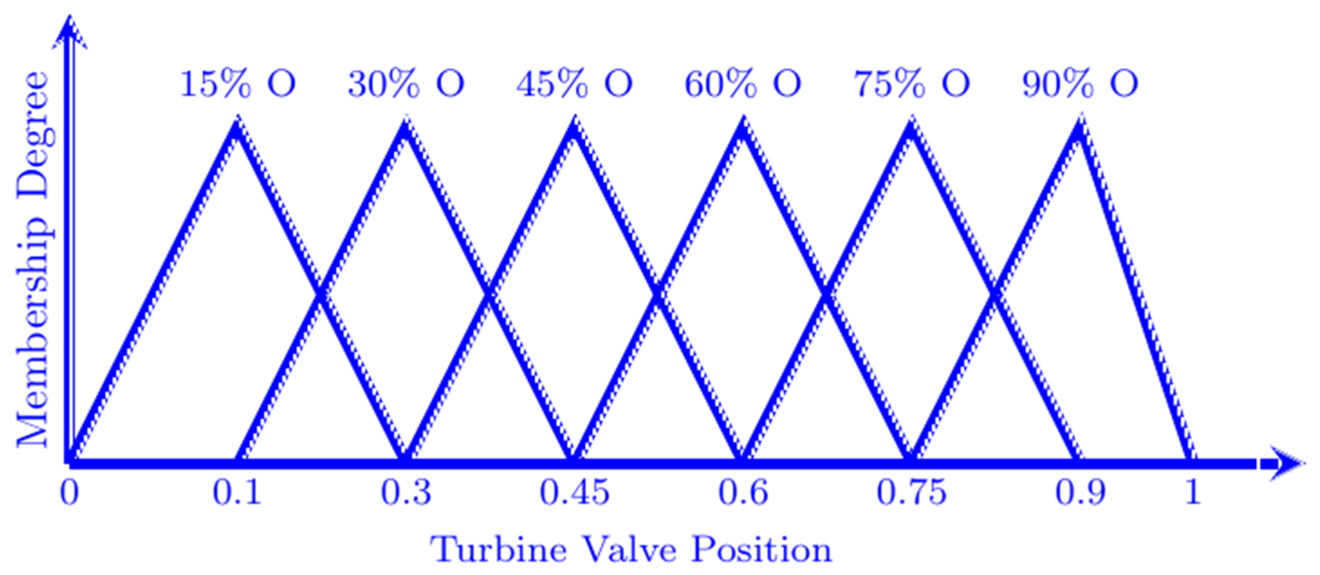
3. Fuzzy Logic Control

Lotfi Asker Zadeh introduced the fuzzy logic approach in 1965 [26]. It comprises three steps: fuzzification, rule-based inference engine, and defuzzification, as depicted in Figure 4. It can be applied to nearly every discipline; it could be used to models whose mathematical modeling is not well defined, and it has been applied widely in LFC and AGC. M. A. R. Shafei, D. K. Ibrahim, and M. Bahaa presented, in [27], a PSO-tuned fuzzy logic controller for the LFC of a two-area power system. The performance of the proposed controller has been validated by comparing its results with those of a recently published PID-P controller, where it achieved less settling time and less undershooting and overshooting values. In [28], T. Hussein and A. Shamekh proposed a gain-scheduling PI fuzzy logic two-level LFC for a two-area power system. This technique eliminates steady-state error and results in good transient response. The results derived from applying the criterion of integral square error (ISE) using MATLAB Simulink show the proficiency of the proposed technique.

B. Khokhar, S. Dahiya, and K. P. S. Parmar proposed, in [29], a novel hybrid fuzzy proportional derivative–tilt integral derivative (FPD-TID) controller for the load frequency control (LFC) analysis of a standalone microgrid. The developed controller has been optimized using a robust chaotic crow search algorithm (CCSA). A. Ghafouri, J. Milimonfared, and G. B. Gharehpetian applied, in [30], Fuzzy-Adaptive Frequency Control to study the effect of microgrids and wind penetration on LFC. The improved hierarchical coordinated control technique has been applied to the IEEE 39-bus system, including microgrids and windfarms. The results validated the developed method’s effectiveness in improving the power quality and the frequency response.

K. Ben Meziane, R. Naoual, and I. Boumhidi presented, in [31], the interval type-2, fuzzy-logic-based, tuned PID controller for AGC of a two-area hydro, gas, and thermal power system with an Advanced Thyristor Controlled Series Capacitor (ATCSC). ITAE is considered as the objective function. The results derived from the proposed algorithm show the efficiency of applying it to obtain stable frequency and load responses. Compared to other controllers, the presented technique demonstrates an excellent damping response. A. Bloul, A. Sharaf, and M. El-Hawary [32] introduced a low-cost flexible AC transmission system (FACTS)-based, flexible fuzzy-logic-controller-tuned arm filter and Green Plug compensation scheme for single-phase nonlinear loads to improve power quality, correct power factor, diminish switching transients, and reduce harmonics.

In Boolean algebra, we only have two states: either true (1) or false (0)—something working 100% or not working at all (0). This can be applied to limited applications, including switches. In real life, many applications do not follow the Boolean algebra rules; numbers like 0.1, 0.15, and 0.2 have some value, whereas they are rounded to zero in Boolean algebra. The speed of objects is not just halted or full speed; there are grades in between, such as the slowest, slower, slow, fast, faster, and the fastest. This is not limited to speed applications but is applied to many cases. In our study, the turbine does not have just two states, open or closed, but can be 5%, 10%, …, and 95% open. Based on that, Boolean algebra does not always suit all applications where we must include all the previous turbine states. To include those scenarios, we applied fuzzy logic, which allowed us to deal with all states between zero and one. A basic example of distinguishing between Boolean algebra and fuzzy logic is illustrated in

Table 1. Comparison between Boolean algebra and fuzzy logic.

Turbine Operation in Boolean Algebra	Turbine Operation in Fuzzy Logic
If (valve == 0) { // Turbine is off } Else { Turbine is on }	If ((valve >= 0) && (valve < 0.25)) { // Turbine is quarter opened } Else if ((valve >= 0.25) && (valve < 0.5)) { //Turbine is half-opened } Else if ((valve >= 0.5) && (valve < 0.75)) { //Turbine is three-quarters opened } Else if ((valve >= 0.75) && (valve < 1.0)) { //Turbine is fully opened }

.

The frequency is the system’s input in all three plants, and the turbine valve is the output. To form the membership functions in the novel GA-fuzzy logic self-tuning approach, we need to specify the range of the inputs and the outputs, where the input in our model is the frequency in Hz and the output is the turbine valve position. Figure 5 and Figure 6 depict the range of the frequency fluctuation and the turbine valve position of the proposed model, respectively. Where OS is overshoot, 0% means there is no overshoot in the response. Where O is open, 0% means the valve is closed, whereas 100% means the valve is fully open.

4. System Configuration

A strategy for the operation of the RES (SORES) has been proposed (Figure 7); this hybrid system comprises a wind energy system, a photovoltaic (PV) system, a biomass gasifier system, and a battery storage system. The wind turbine and solar panels produce DC, so an inverter is required to convert DC into AC. The biomass gasifier produces AC; it is coupled directly to the AC bus. A battery bank storage system will be included in the HES to store surplus energy when generation exceeds demand and supply power when there is deficit energy.

The control system will arrange to meet the sudden demand in the following sequence: When there are enough wind gusts to meet the demand, the wind source will cover the sudden demand. The solar source will cover sudden demand when there is enough solar irradiation to meet the demand. If both wind and solar sources can meet the demand, they can be utilized to provide the load needed. When both wind and solar energy sources cannot meet the demand, biomass energy will be applied to meet the demand. Using this control strategy, we minimize the use of biomass energy to generate power. Figure 8 shows the schematic flowchart of the proposed operation strategy.

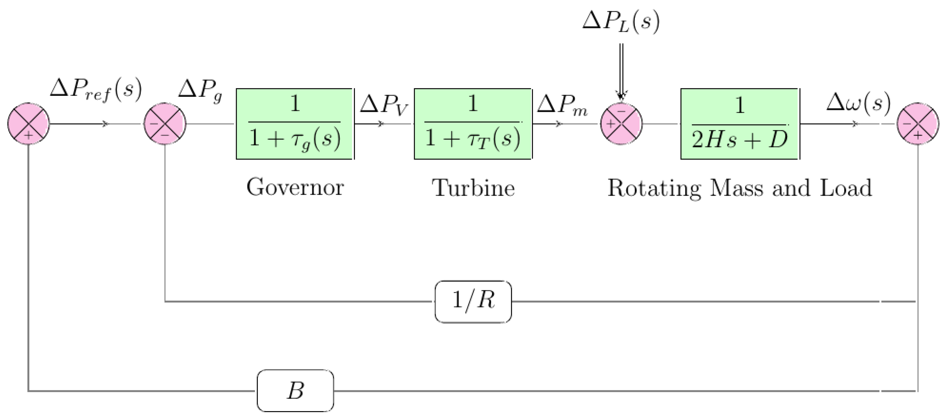
5. Mathematical Modeling of the Components

It is very important to model the system mathematically to size it correctly. The system needs to be optimized under different operating conditions.

5.1. Mathematical Modeling of the Wind Energy System

The electrical power output of a wind energy system at any instant (t) in kW can be calculated using the following equation:

$$P_W=\left\{\begin{array}{cc}0\hfill & V_{Ci}>V\left(t\right)>V_{Co}\\ \frac{\left[\frac{1}{2}\times N_W\times C_P\times {\rho }_a\times A_W\times {\eta }_g\times {\left(V\left(t\right)\right)}^3\right]}{1000}\hfill & V_{Ci}\le V\left(t\right)<V_r\\ P_r\hfill & V_r\le V\left(t\right)\le V_{Co}\end{array}\right.$$

(11)

where $N_W$ is the number of wind turbines in service, CP is the power coefficient of the designated wind turbine model, ${\rho }_a$ is the air density (roughly $1.2 \mathrm{kg}/{\mathrm{m}}^3$), AW is the swept area of the wind turbine rotor, ${\eta }_g$ is the generator efficiency of the wind power system (roughly 90%), $P_r$ is the wind turbine rated power, V(t) is the wind speed in (m/s). and $V_{Ci}, V_{Co}$ and $V_r$ are cut-in speed, cut-out speed, and rated speed, respectively.

5.2. Mathematical Modeling of the Photovoltaic System

The power output of the solar photovoltaic can be obtained using the following equation:

$$P_{PV}\left(t\right)=C_{PV}\times D_{PV}\times \frac{Q_{PV} \left(t\right)}{Q_{PV, STC}}$$

(12)

where $C_{PV}$ denotes the rated capacity of the photovoltaic system under standard test conditions (STC) and panel efficiency of 14%, $D_{PV}$ is a derating factor of the PV array that is used to consider reduced output under real-world conditions like dust, shadow, etc. (80%), $Q_{PV }\left(t\right)$ represents solar irradiance incident on PV array in $\mathrm{kW}/{\mathrm{m}}^2$, and $Q_{PV, STC}$ is the solar radiation at STC ($1 \mathrm{kW}/{\mathrm{m}}^2$).

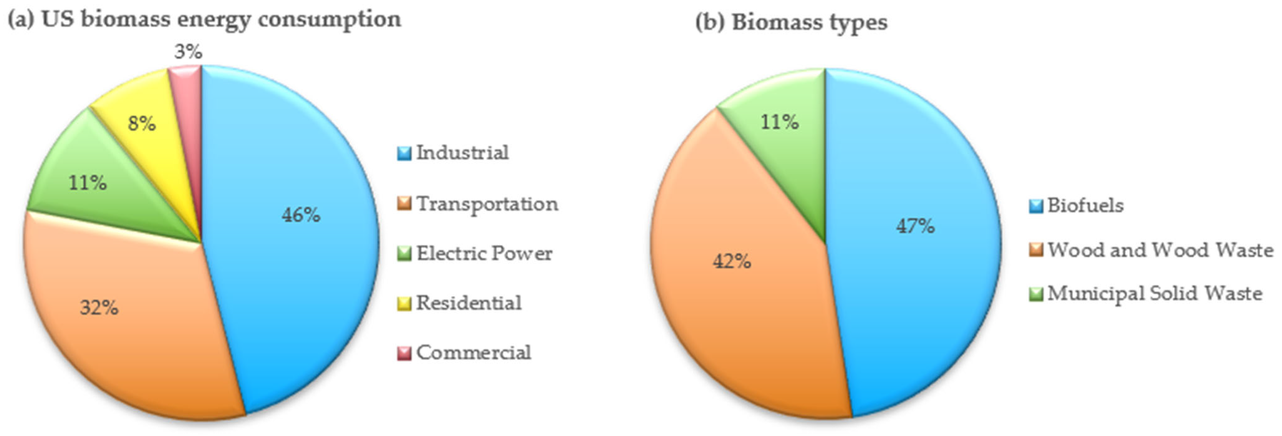
5.3. Mathematical Modeling of the Biomass Gasifier System

The hourly power output obtained from the biomass gasifier system P_Bm (t) in kW can be computed using the following equation:

$$P_{Bm }\left(t\right)=\frac{Q_{Bm}\times C{V}_{Bm}\times {\eta }_{Bm}\times 1000}{365\times 860\times H_D}$$

(13)

where $Q_{Bm }$ is the annual available amount of biomass in (ton/yr), $C{V}_{Bm}$ is biomass calorific value in $\mathrm{kcal}/\mathrm{kg}$, ${\eta }_{Bm}$ is the biomass to electricity overall conversion efficiency of the biomass gasifier (20%), and $H_D$ represents the biomass gasifier systems’s operating hours per day.

5.4. Mathematical Modeling of the Battery Bank Storage System

Battery banks are often installed in the wind and PV models. They save energy when they produce surplus energy and supply the network with energy when the system has a deficit. During charging, the battery bank capacity at time (t) can be expressed using the following equation:

$$U_{Bt}\left(t\right)=U_{Bt}\left(t-1\right)+\left[\left(U_{s-AC}\left(t\right)\times {\eta }_{rec}\times {\eta }_{chg}\right)+\left(U_{s-DC}\left(t\right)\times {\eta }_{chg}\right)\right]$$

(14)

where $U_{Bt}\left(t-1\right)$ is the energy that is stored in the battery bank in (kWh); $U_{s-AC}\left(t\right)$ is the energy surplus from the AC source, the biomass gasifier in this case; $U_{s-DC}\left(t\right)$ is the energy surplus from the DC source, the PV array, and the wind energy based system after serving the load; ${\eta }_{rec}$ is the rectifier efficiency (90%); and ${\eta }_{chg}$ is the battery bank charging efficiency (90%).

While discharging, the battery bank capacity at time (t) can be calculated from the following equation:

$$U_{Bt}\left(t\right)=U_{Bt}\left(t-1\right)-\left[\frac{U_{nl}\left(t\right)}{{\eta }_{inv}\times {\eta }_{dchg}}\right]$$

(15)

where $U_{nl}\left(t\right)$ is the load net deficit, which RES does not serve; ${\eta }_{inv}$ is the inverter efficiency (95%); and ${\eta }_{dchg}$ is the battery discharging efficiency (100%).

6. Problem Formulation

The problem formulation contains the objective functions and the constraints. The main objective function is to minimize ITAE and the NPC of the hybrid system. The total NPC of the hybrid system represents the present value of all the project costs during its lifetime minus the present value of all the revenue earned over its lifetime. The costs considered here include capital costs, replacement costs, fuel costs, O&M costs, and emissions penalties. The revenues include the biomass gasifier, diesel generator, and salvage values of batteries. If the system is grid-connected, the costs of purchasing electricity from the grid will be added to all project costs, and selling power to the grid will be added to revenue costs.

The total net present cost is calculated using HOMER, as follows:

$$C_{NPC}=\frac{C_{yt}}{CRF\left(i_r,R_p\right)}$$

(16)

where $C_{NPC}$ is the total net present cost in USD, $C_{yt}$ is the total annualized cost in USD/year, CRF is the capital recovery factor, $i_r$ is the interest rate in %, and $R_p$ is the project’s lifetime in years.

CRF transforms the system components’ present value into equal increments of annual payments over the project lifetime and is computed as follows:

$$CRF\left(i_r,R_p\right)=\frac{i_r{\left(1+i_r\right)}^{n_{pl}}}{{\left(1+i_r\right)}^{n_{pl}}-1}$$

(17)

where $i_r$ is the yearly real interest rate and $n_{pl}$ is the project lifetime. The yearly real interest rate is the discount rate used to switch between one-time costs and annualized costs, while the nominal interest rate is a bank loan.

6.1. Constraints

The HES can be optimized using the following constraints.

6.1.1. Power Reliability Constraints

Equation (18) depicts the annual capacity shortage ($F_{CS}$):

$$F_{CS}=\frac{E_{CS}}{E_D}$$

(18)

where $F_{CS}$ is the annual capacity shortage and $E_{CS}$ is the total capacity shortage of a year.

6.1.2. Battery Bank Storage Limits

In any instance (t), the battery bank storage falls into the following constraint:

$$E_{Btmin}\le E_{Bt}\left(t\right)\le E_{Btmax}$$

(19)

where $E_{Btmin}$ and $E_{Btmax}$ are the battery bank storage’s minimum and maximum capacity, respectively. The following equation represents $E_{Btmin}$ and $E_{Btmax}$:

$$E_{Btmin}=\frac{N_{Bt}{V}_{Bt}{S}_{Bt}}{1000}\times S{C}_{min},$$

(20)

$$E_{Btmax}=\frac{N_{Bt}{V}_{Bt}{S}_{Bt}}{1000}\times S{C}_{max}$$

(21)

where $N_{Bt}$, $V_{Bt}$, $S_{Bt}$, $S{C}_{min},$ and $S{C}_{max}$ are the number of batteries, the battery voltage in (V), the battery capacity in Ampere Hour (AH), the minimum state of charge, and the maximum state of charge, respectively.

6.1.3. Lower and Upper Bounds

The wind, solar, and battery bank storage systems are subject to the following constraints:

$$0\le P_{PV}\left(t\right)\le say \left(100\right), where P_{PV}=Integer,$$

(22)

$$0\le N_{WT}\left(t\right)\le say \left(20\right), where N_{WT}=Integer,$$

(23)

$$0\le N_{Bt}\left(t\right)\le say \left(200\right), where N_{Bt }=Integer.$$

(24)

6.1.4. Excess Electricity

When the total electricity generation exceeds demand and batteries reach their maximum storage capacity, we are in the excess electricity stage. The following equation estimates excess electricity in (kWh/yr):

$$P_{EH}=\left\{\begin{array}{c} P_G\left(t\right)-P_D\left(t\right), \hspace{1em}{P}_G\left(t\right)>P_D\left(t\right) and E_{Bt}\left(t\right)=E_{Btmax}\hfill \\ 0, otherwise\hfill \end{array}\right.,$$

(25)

$$P_G\left(t\right)=P_{Bm}\left(t\right)+{\eta }_{inv}\times \left[P_W\left(t\right)+P_{PV}\left(t\right)\right],$$

(26)

$$E_{EY}={\displaystyle \sum }_{t=1}^{8760}{P}_{EH}\left(t\right)$$

(27)

where $P_{EH}\left(t\right)$, $P_G\left(t\right)$, $P_D\left(t\right),$ and $E_{EY}$ represent the hourly excess power in (kW), the total hourly generation from all applied resources in (kW), the hourly power demand in (kW), and the annualized excess electricity in kWh/yr.

6.2. Optimization

Meta-heuristic optimization techniques have become very popular recently. The very well-known ones are Ant Colony Optimization (ACO) [33], GA [34], and PSO [35].

6.2.1. Meta-Heuristic Classes

Meta-heuristics can be divided into two main classes:

• Single-solution based: in Simulated Annealing (SA) [36], for example, the search process starts with one candidate solution and then improves over the course of iterations.
• Population based: They execute the optimization using a set of solutions (population). The search process starts with a random initial population (multiple solutions), which is enhanced over the course of iterations. Swarm Intelligence (SI) is one of the most popular branches of the population-based meta-heuristics. The most popular SI techniques are ACO, Artificial Bee Colony (ABC) [37], and PSO.

6.2.2. Meta-Heuristics Categories

Meta-heuristics can also be categorized into three main classes:

• Evolutionary algorithms (EAs): these algorithms are often inspired by natural concepts of evolution, such as GA and differential evolution (DE) [38].
• Physics based: they mimic physical rules, such as Gravitational Local Search (GLSA) [39], Charged System Search (CSS) [40], Central Force Optimization (CFO) [41], and the Black Hole (BH) algorithm [42].
• SI algorithms: They often mimic the social behavior of swarms, herds, and flocks in nature. Some of the algorithms are PSO, ACO, the ABC and the Bat-inspired Algorithm (BA) [43], and Grey Wolf Optimization (GWO) [44]. According to the No Free Lunch (NFL) theorem, no meta-heuristic can solve all optimization problems. Some algorithms may show promising results on a set of issues, but the same optimization technique may show poor performance on a different set of problems.

This work uses the Hybrid Optimization Model for Electric Renewables (HOMER) Pro Version 3.16.2 software to determine the NPC and the LCOE, and the GA-fuzzy logic self-tuning technique is applied to optimize the ITAE in our AGC model.

6.3. Algorithms Applied for AGC:

Many heuristic optimization algorithms range from straightforward “trial and error” methods to intricate algorithms like evolutionary algorithms. Both the implementation and use of the techniques are simple. The problem’s mathematical formulation is flexible. GA, PS, SA, PSO, and GA-fuzzy logic self-tuning techniques are applied to our model; Figure 9 illustrates the flowchart of our novel hybrid GA-fuzzy logic self-tuning technique.

GA-Fuzzy Logic Self-Tuning Algorithm Procedure:

(1)

Set the values of ω and $P_{tl}$.

(2)

Obtain the values of ω and $P_{tl}$, then calculate $\Delta \mathsf{\omega }$ and $\Delta P_{tl}$.

(3)

Once the values of $\Delta \mathsf{\omega }$ and $\Delta P_{tl}$ are determines, decide the control action to be made.

(4)

Send the control actions to all three plants and calculate ITAE using the GA-fuzzy algorithm.

(5)

Use a fixed-length chromosome to represent the problem variable domain. Select the size of the chromosomal population N, the crossover probability $P_c$, and the mutation probability $P_m$.

(6)

Establish a fitness function to gauge each chromosome’s effectiveness within the issue domain. The fitness function establishes the basis for choosing which chromosomes to mate with during reproduction.

(7)

Generate a starting population of size N chromosomes randomly $\left(x_1, x_2,\dots ,x_N\right)$.

(8)

Determine the fitness value of every single chromosome: $f_{\left(x1\right)},\dots ,f_{\left(xn\right)}$.

(9)

Choose a pair of chromosomes from the existing population to mate with. Parent chromosomes are chosen based on fitness-related probability. Fitter chromosomes are more likely to be selected for mating than less suitable ones.

(10)

Apply the crossover and mutation genetic operators to produce a pair of offspring chromosomes.

(11)

Insert the progeny chromosomes into the newly formed population.

(12)

Step 9 should be repeated until the size of the new chromosomal population equals that of the original population, N.

(13)

Use the new (offspring) chromosomal population in place of the original (parent) population.

(14)

Repeat from step 8 until the termination creation is fulfilled. Examine whether the solution that satisfies the equality constraint is feasible.

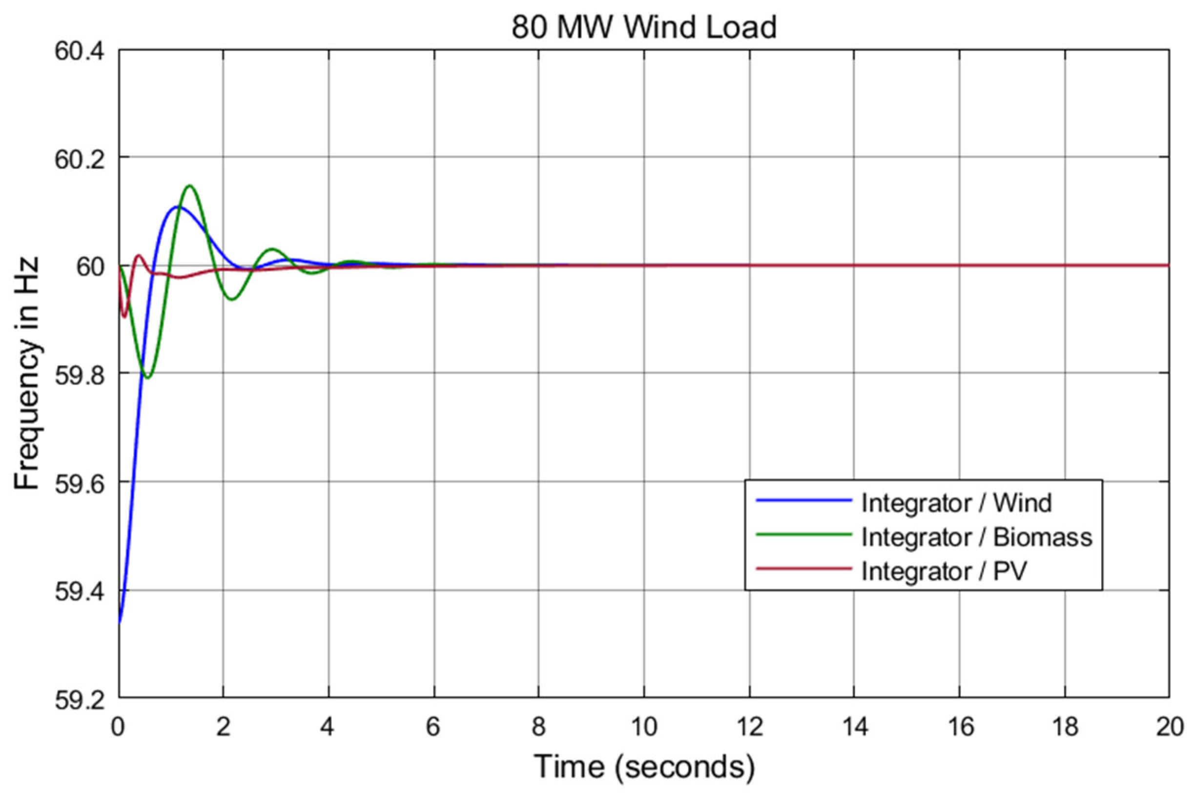
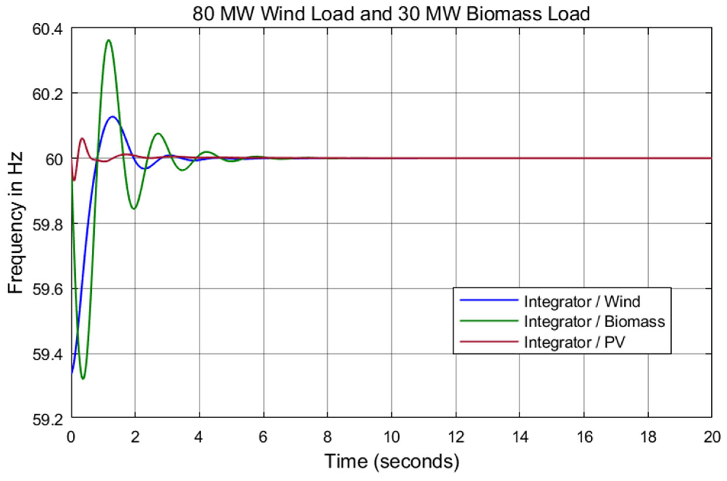
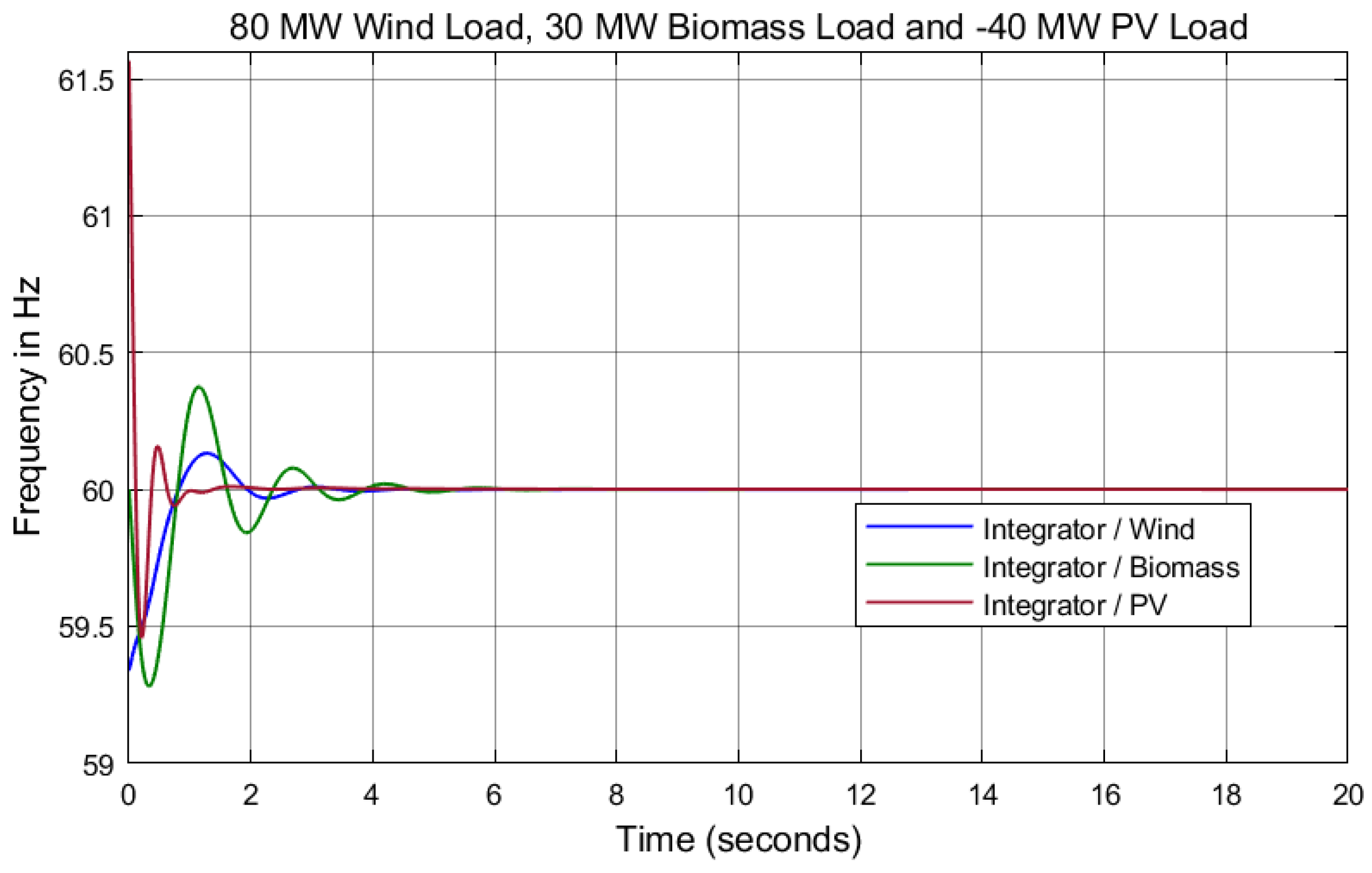
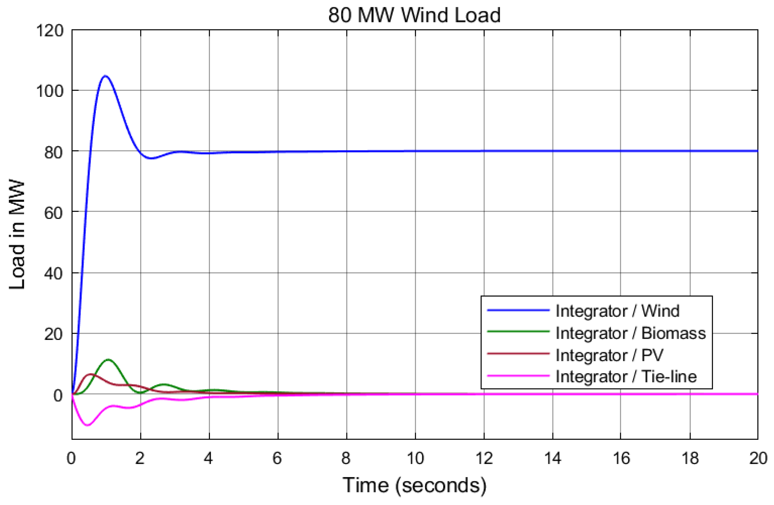
7. Results and Discussion

A multi-area power plant transfer function could be designed similarly to a single-area power plant with the addition of tie-line power flow, see Figure 3. When no extra load demand occurs on the system, the system frequency will be stable, and all three plants will work parallel at the nominal frequency of 60 Hz. In this work, some loads are added to the wind, biomass, and solar power plants to test the system. In this work, the frequency in Hz is measured in the three plants, and the mechanical power flow in MW in all three plants is measured as well, in addition to measuring the tie-line power flow in MW. In the case of any sudden load occurring in any of the three power plants, the system frequency will fluctuate, and the power plant will augment its power generation to meet the increased load demand.

If the system is not designed professionally, all three power plants will increase their generation to meet the demand, and the tie-line will provide the power; consequently, the frequency may vary between 59 Hz and 61 Hz, or worse. In practice, when an unexpected demand occurs in a specific plant, that power plant must absorb that demand; the other plants must not sense it, and the tie-line power should have 0 MW power flow.

To overcome such scenarios, an integrator is added to the model. As can be seen from Figure 10 and Figure 13, when an increment load of 80 MW is added to the wind power plant, the whole load is supplied from that source; the biomass power plant, the photovoltaic power plant, and the tie-line supply 0 MW of load and the frequency is kept steady at 60 Hz.

When adding another increment load of 30 MW to the biomass power plant in addition to the existing 80 MW load on the wind power plant, the designated power plants cover the demand, the photovoltaic power plant and the tie-line supply 0 MW of load, and the frequency is kept steady at 60 Hz (see Figure 11 and Figure 14).

To test the system’s functionality, a sudden load decrease of −40 MW is applied to the photovoltaic power plant in addition to the existing 80 MW load on the wind power plant and the 30 MW on the biomass power plant. The designated power plants cover the demand, the tie-line supplies 0 MW of load, and the frequency is kept steady at 60 Hz (see Figure 12 and Figure 15).

We obtained the desired results when we added the integrator but with a longer settling time, overshoot, and undershoot, as seen in Figure 10, Figure 11, Figure 12, Figure 13, Figure 14 and Figure 15. To obtain better results, the frequency should be steady in minimal time, with less settling time and less overshooting and undershooting; the PID controller should be added in place of the integrator.

The PID’s parameters could be tuned manually to obtain good results, but many optimization techniques may promptly give better results. In our model, we applied GA, PS, SA, and PSO to tune the parameters, then applied the novel GA-fuzzy logic self-tuning technique.

Table 2. The PID parameters use different algorithms.

	Parameters	GA	PS	SA	PSO	GA-Fuzzy
Controller I	P	21.5457	20	19.99679	20	30
	I	17.30914	20	13.25205	15.43407	24.08826
	D	3.633331	14.93847	3.751003	3.970836	4.72576
Controller II	P	21.71193	20	6.856002	18.72205	15.95172
	I	29.9966	20	19.9941	17.68945	30
	D	0.029296	0.228512	0.005082	0	0
Controller II	P	27.93593	20	6.517656	20	29.99936
	I	22.96649	20	19.99775	20	27.68385
	D	3.053391	20	1.268777	8.207062	17.06332
Controller IV	P	21.17271	10.18554	19.71834	17.08208	26.20549
	I	5.398859	0.268551	5.126602	4.375707	5.24566
	D	14.78407	0.251951	12.20899	16.78958	27.84191

shows the parameters of the P, I, and D; these parameters are obtained using MATLAB R2017b software.

As is well known, power loads are variable; they fluctuate continuously at every moment. On the contrary, PID controllers have shortcomings in their parameters as they cannot be tuned online to accommodate load changes. As a result, PID controllers cannot deliver the appropriate response for every load fluctuation. This means that some concessions must be taken to test the PID controller’s performance in all scenarios with various settings.

In control theory, the overshoot occurs when a signal exceeds its stability target, while undershoot is the opposite. When we applied the integrator, the frequency response went up to 61.5 Hz and down to 59.3 Hz, and it took about 4 s until it became stable at 60 Hz. When the frequency recovers to 60 Hz, the load demand will be covered by the designated generation plants. A 1.2 Hz fluctuation is unacceptable from an engineering point of view, and other steps must be taken to improve the frequency and the power output. In the following section, the PID controller is applied instead of the integrator, and the results obtained are compared. Applying the PID controller and adjusting its P, I, and D gain parameters, according to Table 2, makes the system stable faster with less overshoot and undershoot, as seen in Figure 16, Figure 17, Figure 18, Figure 19, Figure 20 and Figure 21 and

Table 3. Comparison of values of rise time between the applied algorithms.

	Rise Time
	Integrator	GA	PS	SA	PSO	GA-Fuzzy
$\Delta F_W$	0.6383	5.94 × 10−4	1.64 × 10−4	2.57 × 10−4	6.32 × 10−4	3.75 × 100
$\Delta F_B$	1.21 × 10−5	4.97 × 10−7	0.0069	6.56 × 10−7	4.94 × 10−8	4.14 × 10−2
$\Delta F_{PV}$	0.0801	5.21 × 10−4	1.37 × 10−4	2.44 × 10−4	5.69 × 10−4	8.37 × 10−6
$\Delta P_{T-line}$	2.80 × 10−5	1.40 × 10−3	1.91 × 10−4	1.90 × 10−3	9.71 × 10−4	2.00 × 10−3
$AC{E}_W$	0.3718	3.91 × 10−4	8.59 × 10−5	4.14 × 10−4	3.43 × 10−4	5.48 × 10−5
$AC{E}_B$	3.39 × 10−1	1.63 × 10−2	1.65 × 10−2	3.58 × 10−2	1.89 × 10−2	2.50 × 10−3
$AC{E}_{PV}$	0.768	1.11 × 100	1.11 × 100	1.12 × 100	1.11 × 100	3.01 × 10−1

,

Table 4. Comparison of values of settling time between the applied algorithms.

	Settling Time
	Integrator	GA	PS	SA	PSO	GA-Fuzzy
$\Delta F_W$	2.6067	0.5813	0.7642	0.7443	0.7738	6.3051
$\Delta F_B$	4.389	1.6777	2.4703	1.165	2.3389	3.0165
$\Delta F_{PV}$	0.7863	0.0863	0.0429	0.0937	0.0951	5.5882
$\Delta P_{T-line}$	7.45	5.1307	0.1585	8.9649	4.2436	10.846
$AC{E}_W$	3.1814	2.1047	2.0722	2.048	2.1251	6.2576
$AC{E}_B$	4.906	0.2603	0.1037	0.489	0.2915	0.0056
$AC{E}_{PV}$	2.8787	2.0544	2.0973	2.1189	2.015	3.5384

,

Table 5. Comparison of values of peak overshoot between the applied algorithms.

	Peak Overshoot
	Integrator	GA	PS	SA	PSO	GA-Fuzzy
$\Delta F_W$	9.29 × 10−6	1.35 × 107	2.30 × 10−5	6.04 × 10−7	0.00 × 100	0
$\Delta F_B$	0.0142	1.22 × 10−4	3.81 × 10−4	0.0152	8.65 × 10−6	0
$\Delta F_{PV}$	0.0341	0.0222	0.0589	0.0357	0.0042	0
$\Delta P_{T-line}$	2.16 × 103	1.19 × 106	6.79 × 106	1.93 × 106	1.04 × 104	1.05 × 101
$AC{E}_W$	35.2413	3.57 × 101	3.78 × 101	35.9763	3.85 × 10−1	0
$AC{E}_B$	53.2843	3.07 × 101	3.06 × 101	51.2822	1.18 × 100	0
$AC{E}_{PV}$	0	9.36 × 10−2	0.00 × 100	0.0048	3.94 × 100	0

and

Table 6. Comparison of values of peak undershoot between the applied algorithms.

	Peak Undershoot
	Integrator	GA	PS	SA	PSO	GA-Fuzzy
$\Delta F_W$	0	2.54 × 104	0	0	0	9.29 × 10−6
$\Delta F_B$	0	0	0	0	0	0.0142
$\Delta F_{PV}$	0	0	0	0	0	0.0341
$\Delta P_{T-line}$	7.71 × 103	1.90 × 105	7.53 × 106	5.2 × 106	4.41 × 104	2.16 × 101
$AC{E}_W$	0	0	0	0	0	0.0241
$AC{E}_B$	6.2888	2.2179	2.3081	4.0984	1.0004	0.2843
$AC{E}_{PV}$	3.7812	1.542	1.9664	5.8355	0	0

.

Because all the algorithms give very similar responses except for the novel GA-fuzzy logic self-tuning algorithm, we are content with demonstrating the frequency and the mechanical load responses when the PID parameters are tuned using the GA algorithm to limit the pages. Figure 16, Figure 17 and Figure 18 depict the frequency response when the PID parameters are tuned using the GA algorithm; as shown in Figure 16, when the wind power plant experienced a sudden load of 80 MW, it experienced some fluctuation in the frequency between 59.98 Hz and 60.01 Hz. It took about 2.5 s until the system became stable. When a sudden 30 MW load occurred in the biomass power plant (Figure 17) and a decrement −40 MW load occurred in the photovoltaic power plant (Figure 18), the frequency experienced more fluctuation between 59.96 Hz and 60.02 Hz, and it took about 3 s until the system became stable.

Figure 19, Figure 20 and Figure 21 depict the mechanical load response when the PID parameters are tuned using the GA algorithm; as shown in Figure 19, when the wind power plant experienced a sudden load of 80 MW, and because the frequency was not fixed at 60 Hz, the biomass power plant provided about 105 MW of power to meet the sudden load demand and took about 3 s to supply 80 MW of load at 60 Hz frequency. Adding an increment of 30 MW sudden load (Figure 20) and a decrement of −40 MW sudden load (Figure 21) to the biomass power plant and the photovoltaic power plant, respectively, made the system experience some fluctuation for about 3 s. Because of the instability in the frequency, the biomass power plant and the photovoltaic power plant provided more than the requested load for about 3 s. When the frequency became stable at 60 Hz, all three power plants provided the load needed.

PID controllers provide compromised responses for all scenarios. Nevertheless, they may not offer the best solution for every condition. On the other hand, applying the GA-fuzzy logic self-tuning approach, when the rules for each circumstance are established separately, may offer the optimum response for each case. The best response might be obtained by applying the novel GA-fuzzy logic self-tuning control compared to other methods.

Figure 22, Figure 23 and Figure 24 depict the frequency response when the PID parameters are tuned using the novel GA-fuzzy logic self-tuning algorithm; as shown in Figure 22, when the wind power plant experienced a sudden load of 80 MW, it experienced a very slight change in the frequency between 59.9985 Hz and 60 Hz, which is about 0.0015 Hz difference. Adding an increment of 30 MW sudden load (Figure 23) and a decrement of −40 MW sudden load (Figure 24) to the biomass power plant and the photovoltaic power plant, respectively, made the system again experience a very slight change in frequency between 59.9942 Hz and 60.0025 Hz, which is about 0.0083 Hz difference.

Figure 25, Figure 26 and Figure 27 depict the mechanical load response when the PID parameters are tuned using the novel GA-fuzzy logic self-tuning algorithm. Figure 25, Figure 26 and Figure 27 show that the system promptly acted on the power demand, which the designated power plants immediately covered. In comparing the results derived from the proposed novel GA-fuzzy logic self-tuning model with some modern heuristic optimization techniques, it is found that this model demonstrates superior frequency response, overshoot, undershoot, and settling time.

After the model is checked to meet the sudden demand, it will be programmed to work according to the proposed strategy of operation shown in Figure 7. Even though biomass is considered renewable energy, it emits CO₂ into the atmosphere, so the program is written to lower utilizing it. When there is enough wind speed or solar irradiation to meet the load demand, the wind or solar energy sources will cover the sudden demand. Because wind and solar energies are intermittent, they cannot always cover the demand. So, when there are not enough wind gusts or solar irradiation to meet the demand, the biomass power plant will cover it.

8. Conclusions and Future Work

8.1. Conclusions

In this work, the PID controller’s parameters are tuned using different heuristic-based optimization techniques and the proposed novel GA-fuzzy logic self-tuning model to control the frequency and the mechanical load of a multi-area renewable energy system. The proposed method has effectively minimized the search area and improved the system’s accuracy.

The novelty of this work is adding biomass energy to the study of the AGC and the proposed hybrid GA-fuzzy self-tuning technique. The program was written to lower the use of biomass in the presence of wind and solar energy sources. The system was tested by adding a sudden 80 MW load to the wind power plant and checking the frequency and the mechanical load responses. Then, we added another 30 MW sudden load to the biomass power plant and checked the frequency and mechanical load responses. After checking the system with increased sudden demands, a sudden decline in the demand was applied to the photovoltaic power plant.

Good results are obtained when the integrator is applied as a controller. Heuristic-based optimization techniques, namely GA, PS, SA, and PSO, gave better settling time, overshoot, and undershoot results. From the literature, it is found that PID controllers are limited by parameter tuning and cannot modify all their parameters at once for every situation. As a result, the PID controller offers a system response that is either compromised or sufficient. It falls short of providing the optimal reaction for all operational settings. The novel GA-fuzzy logic self-tuning algorithm has been applied to tune the PID parameters to overcome such disadvantages and obtain optimum results. Figure 22, Figure 23, Figure 24, Figure 25, Figure 26 and Figure 27 show that the novel GA-fuzzy logic self-tuning algorithm provided optimum settling time, overshoot, and undershoot results.

By comparing the novel GA-fuzzy logic self-tuning algorithm with the other heuristic-based optimization techniques applied, we conclude that the proposed model offers the optimum response for all operational conditions. Applying renewable energy sources in place of conventional energy sources helps meet the 2050 commitment of lowering the carbon footprint or zero carbon emissions. A strategy of operation is introduced to specify which energy source would be applied at any instance.

8.2. Future Work

As an extension for the proposed work, the following steps are considered:

A novel hybrid multi-objective optimized technique will be proposed and used to add more constraints. Thus, a plan is made to create an application for management and optimization purposes to lower the cost of energy and the carbon footprint and improve the system’s performance.

Future work will also consider load seasonality and geographic dependence, which could significantly improve wind speed accuracy and solar irradiance prediction. Most analyses and validations usually concern historical data about meteorological, wind speed, and solar irradiance data linked to specific geographical locations. Future work will consider employing real-time data from neighboring stations. Such an approach could yield a more advanced strategy to design a dynamic energy management platform that includes and compares real-world data with forecasted data.

References

1. Saadat, H. Power System Analysis; WCB/McGraw-Hill: Boston, MA, USA, 1999; Volume 2, pp. 567–576. [Google Scholar]
2. US Energy Information Administration. Biomass Explained. Eia.gov. EIA. 2023. 30 June 2023. Available online: https://www.eia.gov/energyexplained/biomass/ (accessed on 15 January 2024).
3. Ali, G.; El-Hawary, M. Generating Heat and Power from Biomass—An Overview. In Proceedings of the 2019 IEEE Canadian Conference of Electrical and Computer Engineering (CCECE), Edmonton, AB, Canada, 5–8 May 2019. [Google Scholar] [CrossRef]
4. Ali, G.; Aly, H.H.; Little, T. A Modified Ant Lion Optimization Technique for Economic Emission Dispatch Including Biomass. In Proceedings of the 2021 International Conference on Electrical, Communication, and Computer Engineering (ICECCE), Kuala Lumpur, Malaysia, 12–13 June 2021. [Google Scholar] [CrossRef]
5. Aly, H.H. Dynamic modeling and control of the tidal current turbine using DFIG and DDPMSG for power system stability analysis. Int. J. Electr. Power Energy Syst. 2016, 83, 525–540. [Google Scholar] [CrossRef]
6. Jagatheesan, K.; Anand, B.; Samanta, S.; Dey, N.; Ashour, A.S.; Balas, V.E. Design of a proportional-integral-derivative controller for an automatic generation control of multi-area power thermal systems using firefly algorithm. IEEE/CAA J. Autom. Sin. 2019, 6, 503–515. [Google Scholar] [CrossRef]
7. Gupta, D.K.; Jha, A.V.; Appasani, B.; Srinivasulu, A.; Bizon, N.; Thounthong, P. Load Frequency Control Using Hybrid Intelligent Optimization Technique for Multi-Source Power Systems. Energies 2021, 14, 1581. [Google Scholar] [CrossRef]
8. Sahu, R.K.; Panda, S.; Padhan, S. A hybrid firefly algorithm and pattern search technique for automatic generation control of multi area power systems. Int. J. Electr. Power Energy Syst. 2015, 64, 9–23. [Google Scholar] [CrossRef]
9. Ghosh, A.; Ray, A.K.; Nurujjaman; Jamshidi, M. Voltage and frequency control in conventional and PV integrated power systems by a particle swarm optimized Ziegler–Nichols based PID controller. SN Appl. Sci. 2021, 3, 314. [Google Scholar] [CrossRef]
10. Barisal, A.; Mishra, S. Improved PSO based automatic generation control of multi-source nonlinear power systems interconnected by AC/DC links. Cogent Eng. 2018, 5, 1422228. [Google Scholar] [CrossRef]
11. Bhagat, S.K.; Saikia, L.C.; Raju, D.K.; Babu, N.R.; Ramoji, S.K.; Dekaraja, B.; Behra, M.K. Maiden Application of Hybrid Particle Swarm Optimization with Genetic Algorithm in AGC Studies Considering Optimized TIDN Controller; Springer: Singapore, 2021; Volume 206. [Google Scholar]
12. Alhelou, H.H.; Golshan, M.E.H.; Fini, M.H. Wind Driven Optimization Algorithm Application to Load Frequency Control in Interconnected Power Systems Considering GRC and GDB Nonlinearities. Electr. Power Compon. Syst. 2018, 46, 1223–1238. [Google Scholar] [CrossRef]
13. Huang, C.; Li, J.; Mu, S.; Yan, H. Linear active disturbance rejection control approach for load frequency control of two-area interconnected power system. Trans. Inst. Meas. Control 2017, 41, 1562–1570. [Google Scholar] [CrossRef]
14. Changmai, H.; Buragohain, M. Optimal Controller Design for LFC in Power System, Smart Innovation, Systems and Technologies; Springer: Singapore, 2021. [Google Scholar] [CrossRef]
15. Karnavas, Y.L.; Nivolianiti, E. Harris hawks optimization algorithm for load frequency control of isolated multi-source power generating systems. Int. J. Emerg. Electr. Power Syst. 2023, 1–17. [Google Scholar] [CrossRef]
16. Shankar, R.; Chatterjee, K.; Bhushan, R. Impact of energy storage system on load frequency control for diverse sources of interconnected power system in deregulated power environment. Int. J. Electr. Power Energy Syst. 2016, 79, 11–26. [Google Scholar] [CrossRef]
17. Çelik, E.; Öztürk, N.; Arya, Y.; Ocak, C. (1 + PD)-PID cascade controller design for performance betterment of load frequency control in diverse electric power systems. Neural Comput. Appl. 2021, 33, 15433–15456. [Google Scholar] [CrossRef]
18. Babu, N.R.; Saikia, L.C.; Bhagat, S.K.; Ramoji, S.K.; Dekaraja, B.; Behra, M.K. LFC of a solar thermal integrated thermal system considering CSO optimized TI-DN controller. In Modeling, Simulation and Optimization: Proceedings of CoMSO 2020; Springer: Singapore, 2021; pp. 323–334. [Google Scholar]
19. Kumar, R.R.; Yadav, A.K.; Ramesh, M. Hybrid PID plus LQR based frequency regulation approach for the renewable sources based standalone microgrid. Int. J. Inf. Technol. 2022, 14, 2567–2574. [Google Scholar] [CrossRef]
20. Pinazo, M.A.; Arias, R.A.; Tarrillo, J.M. Comparison of primary frequency control methods for wind turbines based on the doubly fed induction generator. Wind. Eng. 2022, 46, 1923–1947. [Google Scholar] [CrossRef]
21. Patel, V.; Guha, D.; Purwar, S. Fractional-order Adaptive Sliding Mode Approach for Frequency Regulation in Power System. In Proceedings of the 2021 9th IEEE International Conference on Power Systems (ICPS), Kharagpur, India, 16–18 December 2021. [Google Scholar] [CrossRef]
22. Saxena, P.; Singh, N.; Pandey, A.K. Investigating the frequency fault ride through capability of solar photovoltaic system: Replacing battery via virtual inertia reserve. Int. Trans. Electr. Energy Syst. 2021, 31, e12791. [Google Scholar] [CrossRef]
23. Guo, W.; Yang, J. Stability performance for primary frequency regulation of hydro-turbine governing system with surge tank. Appl. Math. Model. 2018, 54, 446–466. [Google Scholar] [CrossRef]
24. Dash, P.; Saikia, L.C.; Sinha, N. Flower Pollination Algorithm Optimized PI-PD Cascade Controller in Automatic Generation Control of a Multi-area Power System. Int. J. Electr. Power Energy Syst. 2016, 82, 19–28. [Google Scholar] [CrossRef]
25. El-Sehiemy, R.; Shaheen, A.; Ginidi, A.; Al-Gahtani, S.F. Proportional-Integral-Derivative Controller Based-Artificial Rabbits Algorithm for Load Frequency Control in Multi-Area Power Systems. Fractal Fract. 2023, 7, 97. [Google Scholar] [CrossRef]
26. Zadeh, L.A. Is there a need for fuzzy logic? Inf. Sci. 2008, 178, 2751–2779. [Google Scholar] [CrossRef]
27. Shafei, M.A.R.; Ibrahim, D.K.; Bahaa, M. Application of PSO tuned fuzzy logic controller for LFC of two-area power system with redox flow battery and PV solar park. Ain Shams Eng. J. 2022, 13, 101710. [Google Scholar] [CrossRef]
28. Hussein, T.; Shamekh, A. Design of PI Fuzzy Logic Gain Scheduling Load Frequency Control in Two-Area Power Systems. Designs 2019, 3, 26. [Google Scholar] [CrossRef]
29. Khokhar, B.; Dahiya, S.; Parmar, K.P.S. A Novel Hybrid Fuzzy PD-TID Controller for Load Frequency Control of a Standalone Microgrid. Arab. J. Sci. Eng. 2020, 46, 1053–1065. [Google Scholar] [CrossRef]
30. Ghafouri, A.; Milimonfared, J.; Gharehpetian, G.B. Fuzzy-Adaptive Frequency Control of Power System Including Microgrids, Wind Farms, and Conventional Power Plants. IEEE Syst. J. 2018, 12, 2772–2781. [Google Scholar] [CrossRef]
31. Ben Meziane, K.; Naoual, R.; Boumhidi, I. Type-2 Fuzzy Logic based on PID controller for AGC of Two-Area with Three Source Power System including Advanced TCSC. Procedia Comput. Sci. 2019, 148, 455–464. [Google Scholar] [CrossRef]
32. Bloul, A.; Sharaf, A.; El-Hawary, M. An Energy Saving Green Plug Device for Nonlinear Loads. IOP Conf. Ser. Earth Environ. Sci. 2018, 127, 012016. [Google Scholar] [CrossRef]
33. Dorigo, M. Ant colony optimization. Scholarpedia 2007, 2, 1461. [Google Scholar] [CrossRef]
34. John, H. Holland genetic algorithms. Sci. Am. 1992, 267, 44–50. [Google Scholar]
35. Kennedy, J.; Eberhart, R. Particle swarm optimization. In Proceedings of the ICNN’95-International Conference on Neural Networks, Perth, WA, Australia, 27 November–1 December 1995; Volume 4, pp. 1942–1948. [Google Scholar]
36. Kirkpatrick, S. Optimization by simulated annealing. Science 1984, 220, 4598. [Google Scholar]
37. Karaboga, D.; Basturk, B. A powerful and efficient algorithm for numerical function optimization: Artificial bee colony (ABC) algorithm. J. Glob. Optim. 2007, 39, 459–471. [Google Scholar] [CrossRef]
38. Storn, R.; Price, K. Differential evolution—A simple and efficient heuristic for global optimization over continuous spaces. J. Glob. Optim. 1997, 11, 341–359. [Google Scholar] [CrossRef]
39. Webster, B.; Bernhard, P.J. A Local Search Optimization Algorithm Based on Natural Principles of Gravitation; Florida Institute of Technology: Melbourne, FL, USA, 2003. [Google Scholar]
40. Kaveh, A.; Talatahari, S. A novel heuristic optimization method: Charged system search. Acta Mech. 2010, 213, 267–289. [Google Scholar] [CrossRef]
41. Formato, R.A. Central force optimization: A new nature inspired computational framework for multidimensional search and optimization. In Nature Inspired Cooperative Strategies for Optimization (NICSO 2007); Springer: Berlin/Heidelberg, Germany, 2008; pp. 221–238. [Google Scholar]
42. Hatamlou, A. Black hole: A new heuristic optimization approach for data clustering. Inf. Sci. 2013, 222, 175–184. [Google Scholar] [CrossRef]
43. González, J.R.; Sancho-Royo, A.; Pelta, D.A.; Cruz, C. Nature-Inspired Cooperative Strategies for Optimization. In Encyclopedia of Networked and Virtual Organizations; IGI Global: Hershey, PA, USA, 2008; pp. 982–989. [Google Scholar]
44. Mirjalili, S.; Mirjalili, S.M.; Lewis, A. Grey Wolf Optimizer. Adv. Eng. Softw. 2014, 69, 46–61. [Google Scholar] [CrossRef]
Figure 1. AGC of an isolated power system, redrawn from [1].
Energies 17 02000 g001
Figure 2. (a) US biomass energy consumption by sector in 2022. (b) Types of biomasses consumed by sector in the US in 2022.
Energies 17 02000 g002
Figure 3. AGC of the proposed multi-area renewable energy system.
Energies 17 02000 g003
Figure 4. A Block diagram of a fuzzy logic control system.
Energies 17 02000 g004
Figure 5. The model input (Change in Frequency).
Energies 17 02000 g005
Figure 6. The model output (Turbine Valve Position).
Energies 17 02000 g006
Figure 7. Strategy of operation of the RES (SORES).
Energies 17 02000 g007
Figure 8. The schematic flowchart of the proposed strategy of operation.
Energies 17 02000 g008
Figure 9. The flowchart of the GA-fuzzy logic self-tuning algorithm.
Energies 17 02000 g009
Figure 10. Integrator—frequency response—80 MW wind load.
Energies 17 02000 g010
Figure 11. Integrator—frequency response—80 MW wind load and 30 MW biomass load.
Energies 17 02000 g011
Figure 12. Integrator—frequency response—80 MW wind load, and 30 MW biomass load, and −40 MW photovoltaic load.
Energies 17 02000 g012
Figure 13. Integrator—load response—80 MW wind load.
Energies 17 02000 g013
Figure 14. Integrator—load response—80 MW wind load and 30 MW biomass load.
Energies 17 02000 g014
Figure 15. Integrator—load response—80 MW wind load, 30 MW biomass load, and −40 MW photovoltaic load.
Energies 17 02000 g015
Figure 16. GA—frequency response—80 MW wind load.
Energies 17 02000 g016
Figure 17. GA frequency response—80 MW wind load and 30 MW biomass load.
Energies 17 02000 g017
Figure 18. GA—frequency response—80 MW wind load, 30 MW biomass load, and −40 MW photovoltaic load.
Energies 17 02000 g018
Figure 19. GA—load response—80 MW wind load.
Energies 17 02000 g019
Figure 20. GA—load response—80 MW wind load and 30 MW biomass load.
Energies 17 02000 g020
Figure 21. GA—load response—80 MW wind load, 30 MW biomass load, and −40 MW Photovoltaic Load.
Energies 17 02000 g021
Figure 22. GA-fuzzy self-tuning—frequency response—80 MW wind load.
Energies 17 02000 g022
Figure 23. GA-fuzzy self-tuning—frequency response—80 MW wind load and 30 MW biomass load.
Energies 17 02000 g023
Figure 24. GA-fuzzy self-tuning—frequency response—80 MW wind load, 30 MW biomass load, and −40 MW photovoltaic load.
Energies 17 02000 g024
Figure 25. GA-fuzzy self-tuning—load response—80 MW wind load.
Energies 17 02000 g025
Figure 26. GA-fuzzy self-tuning—load response—80 MW wind load and 30 MW Biomass Load.
Energies 17 02000 g026
Figure 27. GA-fuzzy self-tuning—load response—80 MW wind load, 30 MW biomass load, and −40 MW Photovoltaic Load.
Energies 17 02000 g027