Wind-Speed Multi-Step Forecasting Based on Variational Mode Decomposition, Temporal Convolutional Network, and Transformer Model

Abstract

Reliable and accurate wind-speed forecasts significantly impact the efficiency of wind power utilization and the safety of power systems. In addressing the performance enhancement of transformer models in short-term wind-speed forecasting, a multi-step prediction model based on variational mode decomposition (VMD), temporal convolutional network (TCN), and a transformer is proposed. Initially, the Dung Beetle Optimizer (DBO) is utilized to optimize VMD for decomposing non-stationary wind-speed series data. Subsequently, the TCN is used to extract features from the input sequences. Finally, the processed data are fed into the transformer model for prediction. The effectiveness of this model is validated by comparison with six other prediction models across three datasets, demonstrating its superior accuracy in short-term wind-speed forecasting. Experimental findings from three distinct datasets reveal that the developed model achieves an average improvement of 52.1% for R². To the best of our knowledge, this places our model at the leading edge of wind-speed prediction for 8 h and 12 h forecasts, demonstrating MSEs of 1.003 and 0.895, MAEs of 0.754 and 0.665, and RMSEs of 1.001 and 0.946, respectively. Therefore, this research offers significant contributions through a new framework and demonstrates the utility of the transformer in effectively predicting short-term wind speed.

1. Introduction

Wind power is a crucial component of renewable energy sources, representing one of the most viable alternatives to traditional fossil fuels thanks to its eco-friendly properties. This can contribute to decreasing reliance on fossil fuels and mitigating environmental pollution [1]. The Global Wind Energy Council has documented a significant rise in worldwide wind energy capacity, reaching 906 Gigawatt (GW), which represents an annual increase of 9%. The year 2023 was expected to be a milestone, with projections indicating that it would be the inaugural year to witness the addition of more than 100 GW of new capacity across the globe. Their estimates also predict a remarkable expansion of 1221 GW in new capacity from 2023 to 2030 [2]. Accurate predictions of wind speed are essential for the effective management of wind energy generation [3]. Generally, precise forecasts of wind speed can enhance the efficiency of wind resource utilization and reduce the effects of wind energy variability on the stability of the electrical grid, facilitating cost-effective and efficient wind farm operations [4]. Therefore, the importance of accurate wind-speed forecasting is growing in terms of reducing the costs and risks linked to power supply systems [5].

Numerous scholars have endeavored to craft models that yield precise deterministic forecasts of wind speeds. These endeavors have categorized models into four distinct groups: physical, statistical, artificial intelligence (AI)-based, and hybrid models [6,7]. Among these, numerical weather prediction models, such as the weather research and forecasting model [8], are recognized as the most prominent physical models. They predict wind speeds using intricate mathematical equations that factor in meteorological variables like humidity and temperature [9], proving particularly effective for medium-to-long-range forecasts of wind speed [10]. On the other hand, statistical models, such as auto-regressive moving average [11], auto-regressive integrated moving average [12], and vector auto-regression [13], differ from physical models by relying solely on historical data of wind speeds for predictions. These models are adept at capturing the linear variability of wind speeds and excel in forecasting over short-term periods [14]. AI-based models primarily tackle the nonlinear dynamics of wind speed, incorporating simple neural networks (for instance, the back-propagation neural network [15], Elman neural network [16], and multilayer perceptron [17]), along with support vector machines [18] and extreme learning machines [19]. Studies indicate that while deep learning offers suboptimal interpretability, it yields commendable predictive outcomes [20]. Presently, a plethora of deep learning methods have been employed for wind-speed forecasting, such as deep belief networks [21], convolutional neural networks (CNNs) [22], long short-term memory networks (LSTM) [23], gated recurrent units (GRUs) [24], and temporal convolutional networks (TCNs) [25]. TCN-based approaches [26] utilize convolutional kernels to detect temporal changes by moving across the time dimension. Zhang et al. [27] proposed a novel integrated model, blending VMD, the Sparrow Search Algorithm, and bidirectional GRU, that leverages TCNs. It has been observed in various studies that deep learning models often outshine both classical machine learning and statistical models in terms of nonlinear predictive capabilities and feature extraction prowess [28]. The consensus among many scholars is that no single model can fully encapsulate the intricate variations in wind speed, leading to the creation of diverse hybrid models [8]. Zhang et al. [29] developed a hybrid model that merges noise-reduction techniques, optimization strategies, statistical approaches, and deep learning. Neshat et al. [30] introduced a novel hybrid model with a deep learning-based evolutionary approach, featuring a bidirectional LSTM, an efficient hierarchical evolutionary decomposition technique, and an enhanced generalized normal distribution optimization method.

The transformer model has achieved remarkable success in fields such as computer vision and natural language processing, and it is pivotal in bridging the gaps between diverse research domains. In the realm of time series forecasting, transformer-based models have gained prominence due to their multi-head self-attention (MHSA) mechanism. Both the transformer and its adaptations have been proposed for time sequence forecasting tasks [31]. The transformer model, renowned for its effectiveness in the realm of wind-speed prediction, has become a prominent tool in this area. For instance, Wu et al. [32] introduced a novel EEMD-Transformer-based hybrid model for predicting wind speeds. Zhou et al. [33] presented the informer, a model designed for long sequence time forecasts, characterized by a ProbSparse self-attention mechanism for optimal time complexity and memory efficiency. Yang et al. [34] developed a causal inference-enhanced informer methodology employing an advanced variant of the informer model, specifically adapted for long-term time series analysis. Bommidi et al. [35] developed a composite approach that harnesses the predictive strength of the transformer model alongside the analytical prowess of ICEEMDAN to improve wind-speed prediction accuracy. Huang et al. [36] present a new hybrid forecasting model for short-term power load that effectively decomposes power load data into subsequences of varying complexities; employs BPNN for less complex subsequences and transformers for more intricate ones; and amalgamates the forecasts to form a unified prediction. Wang et al. [37] utilized the transformer as a core component to devise an innovative convolutional transformer-based truncated Gaussian density framework, offering both precise wind-speed predictions and reliable probabilistic forecasts. Zeng et al. [38] introduced the DLinear model, which explores the impacts of various design elements of long-sequence time forecast models on their capability to extract temporal relationships. Nie et al. [39] present a novel transformer-based framework for multivariate time series forecasts and self-supervised representation learning. This framework, termed the channel-independent Patch Time Series Transformer (PatchTST), markedly improves long-term forecasting precision.

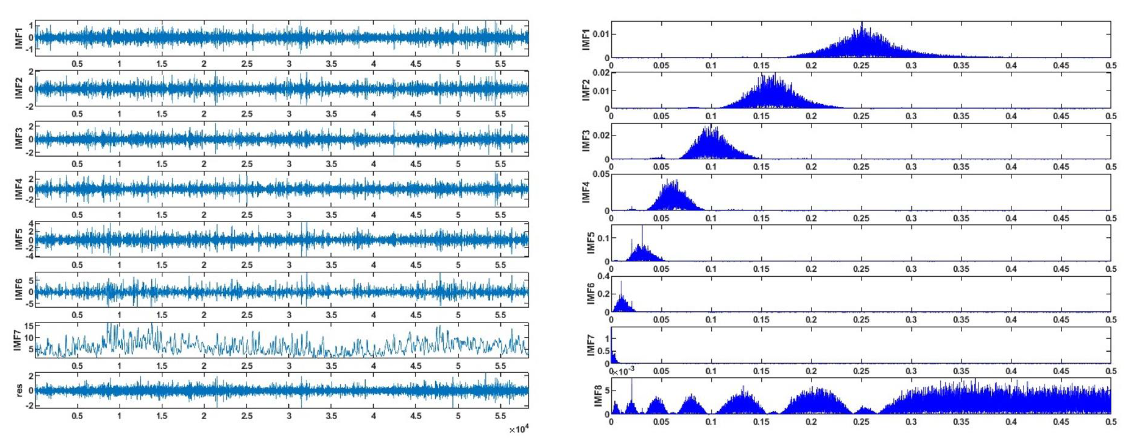
Within the hybrid modeling framework, original wind-speed data are segmented into subseries with distinct frequencies and analyzed individually using specialized models, and their forecasts are amalgamated to produce the final prediction outcome [40]. For instance, Li et al. [41] employed the VMD technique to segregate wind-speed data into intrinsic mode functions (IMFs) of varying frequencies, with each IMF being analyzed through a bidirectional LSTM model. Similarly, Wu et al. [42] utilized VMD to segment wind speed and integrated these segments with multiple meteorological variables to construct a deep-learning model with interpretability. Geng et al. [43] propose a novel prediction framework to enhance short-term power load forecasting accuracy, utilizing a particle swarm optimization (PSO)-enhanced VMD in conjunction with a TCN incorporating an attention mechanism. Zhang et al. [44] proposed a hybrid deep learning model for wind-speed forecasting that combines CNN, bidirectional LSTM, an enhanced sine cosine algorithm, and EDM based on time-varying filtering to improve prediction accuracy. Moreover, Altan et al. [45] presented a predictive model that combines ICEEMDAN decomposition and LSTM, employing grey wolf optimization to fine-tune the weighted coefficients of each IMF for enhanced forecasting precision.

The literature review highlights several existing gaps in the field of wind-speed prediction. Wind-speed prediction studies based on transformers are relatively scarce compared to those based on other deep learning models. This highlights the necessity for a further in-depth exploration of the potential of transformer-based models within the wind-speed prediction domain. In the realm of wind-speed prediction models based on transformers, the majority are designed for long-term forecasting. There is a notable scarcity of models for medium-term, short-term, and ultra-short-term predictions. This indicates a pressing need for the development of transformer-based models that can effectively address medium-term, short-term, and ultra-short-term wind-speed forecasting. Additionally, there is a scarcity of transformer-based wind-speed prediction models that integrate data decomposition algorithms and other models, indicating a need for further exploration of the potential of hybrid forecasting models based on transformers. In response to the aforementioned challenges and needs, this paper introduces a hybrid wind-speed prediction model named DBO-VMD-TCN-Transformer, which integrates Dung Beetle Optimizer (DBO) algorithm-enhanced VMD, TCN, and transformer technologies. The contributions of the study are as follows:

• The model utilizes the DBO algorithm to autonomously determine the most effective decomposition parameters for VMD. This approach significantly reduces signal loss during the decomposition phase and enhances the overall performance of VMD.
• A hybrid forecasting model that combines TCN with transformers is introduced. TCN is employed to extract original wind-speed features, which are then fed into the transformer for multi-step short-term wind-speed prediction.
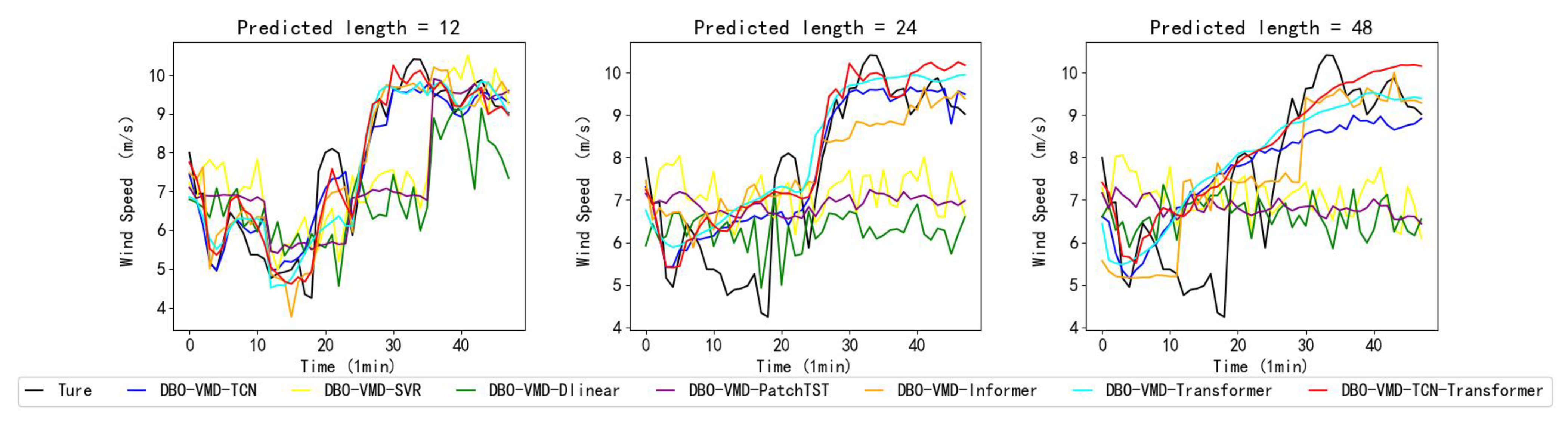
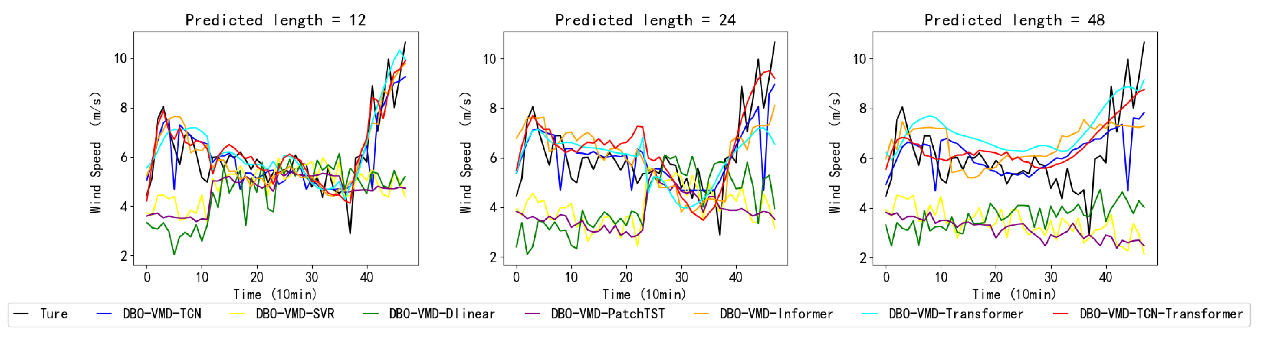
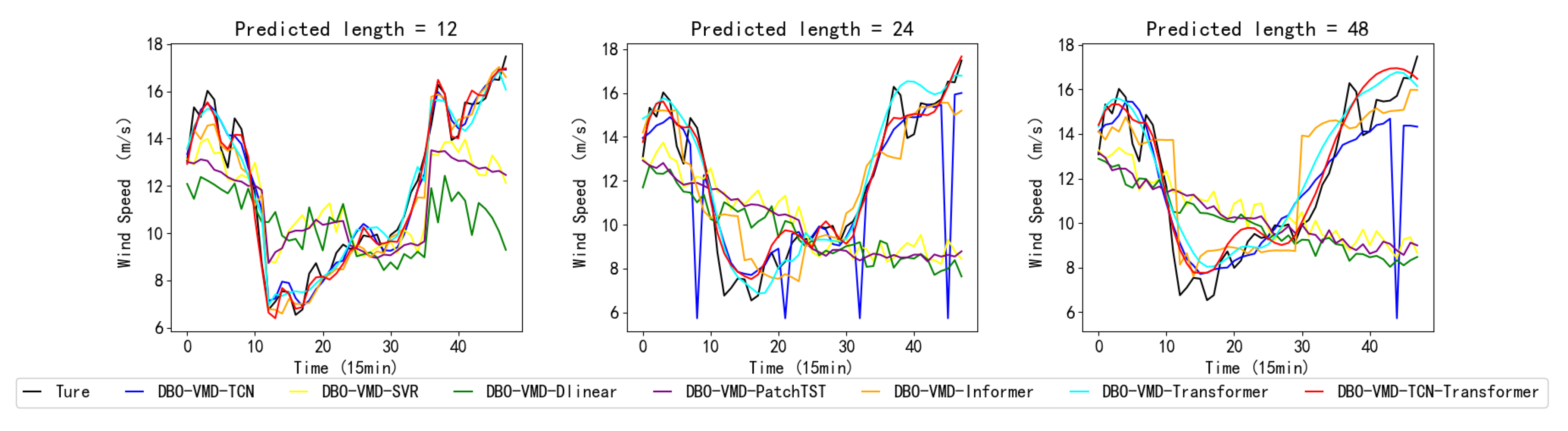
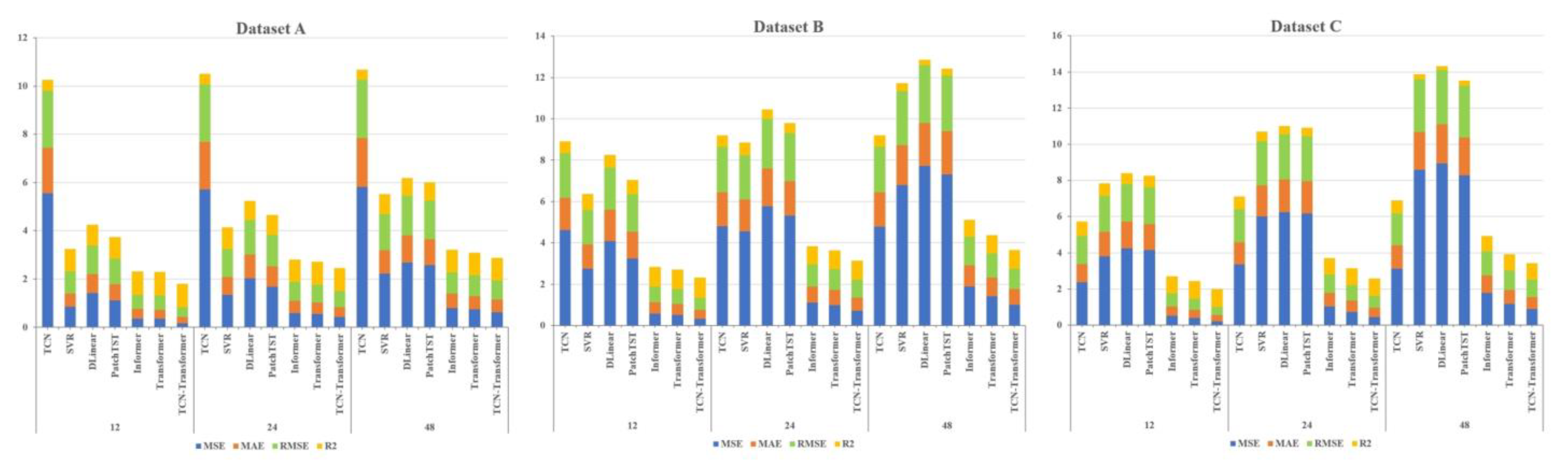
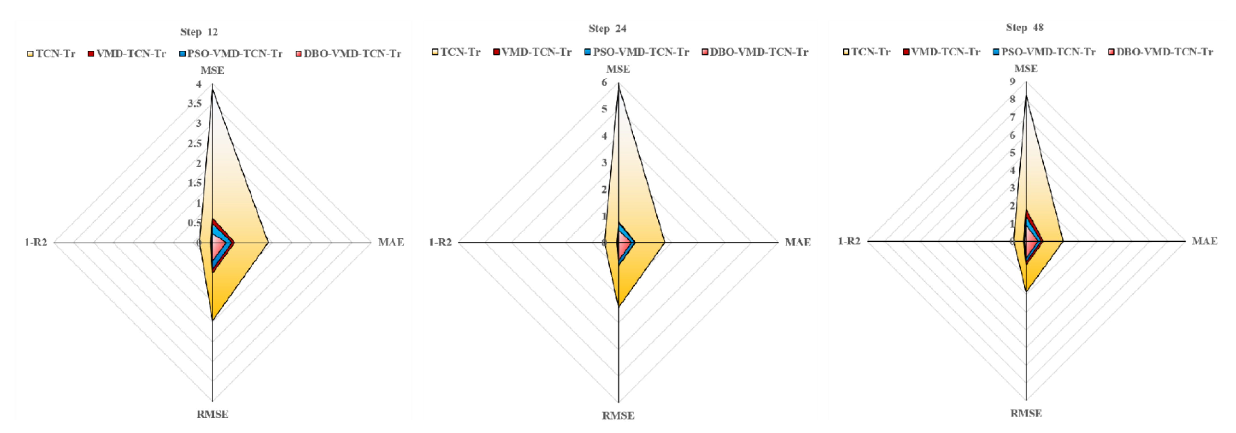
• The DBO-VMD-TCN-Transformer model is compared with TCN, support vector regression (SVR), transformer, informer, PatchTST, Dlinear, VMD-TCN-Informer, and VMD-TCN-PatchTST models. Experimental results on three distinct datasets demonstrate that the developed model outperforms others in all four key metrics of evaluation (MAE, MSE, RMSE, and R²).

2. Methods and Materials

2.1. Flow Chart of the Proposed Model

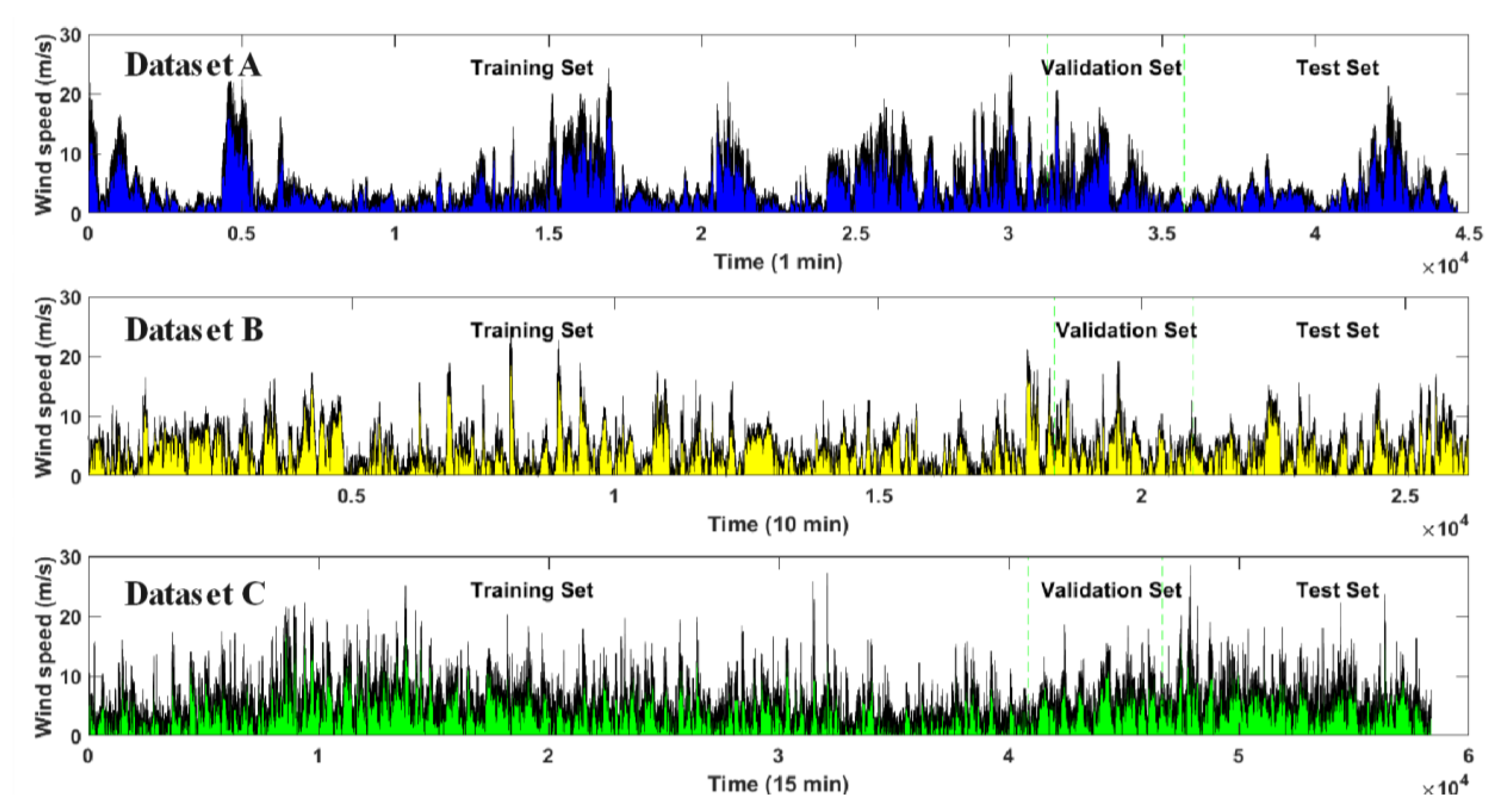
A novel composite forecasting approach is presented, illustrated in Figure 1, which integrates the advantages of DBO-enhanced VMD, TCN, and transformer technologies, concisely referred to as the DBO-VMD-TCN-Transformer. The approach is delineated across three phases: The initial phase involves partitioning the gathered wind-speed data into training, validation, and test groups. Utilizing the DBO algorithm, the optimal parameters for VMD are determined automatically, leading to the segmentation of wind-speed data into various IMFs. In the second phase, the decomposed data are fed into the TCN model to extract features from the high-resolution wind-speed data. These features are subsequently used for multi-step, short-term prediction through a transformer model. The TCN-Transformer architecture is devised to elucidate the complex relationships between historical inputs and forecasted outcomes. The final phase is dedicated to the exposition and analysis of empirical results obtained from three distinct datasets, assessing the framework’s effectiveness and stability via four principal performance metrics (MSE, MAE, RMSE, and R²) in conjunction with the Diebold Mariano (DM) test.

2.2. Variational Mode Decomposition

VMD is a contemporary technique in signal processing that has been increasingly adopted for its effectiveness. It excels in pinpointing the optimal central frequencies and minimizing bandwidth for each mode during analysis, thereby effectively isolating intrinsic mode functions and segmenting the frequency domain [46]. Unlike empirical mode decomposition and wavelet analysis, VMD offers enhanced signal reconstruction capabilities and superior noise immunity. The algorithm decomposes a signal into K distinct frequency bands and stable sub-signals, each characterized by unique oscillatory components with varying frequencies and amplitudes. This approach, optimized through a variational method, seeks to balance the total estimated bandwidths against the minimization of bandwidth sums for each mode, thus achieving an optimal decomposition. The formal definition of VMD in signal decomposing is given by Equation (1).

$$\left\{\begin{array}{l}\underset{\left\{u_k\right\},\left\{{\omega }_k\right\}}{\min }\left\{{\displaystyle {\displaystyle \sum }_{k=1}^K}{\Vert {\partial }_t\left[\left(\delta \left(t\right)+\frac{j}{\pi t}\right)\cdot u_k\left(t\right)\right]e^{-j\omega k^t}\Vert }_2^2\right\}\\ s.t.{\displaystyle {\displaystyle \sum }_{k=1}^K}{u}_k=S\end{array}\right.$$

(1)

In the formulation, the component of mode kth is indicated as $u_k$, and the central frequency for this component is denoted by $\left\{{\omega }_k\right\}$. The representation for the Dirac distribution is given as $\delta \left(t\right)$.

To tackle the original constrained variational formula, the approach integrates a penalty coefficient α along with a Lagrange multiplier λ. This integration effectively shifts the problem from a constrained framework to an unconstrained setting. As a result of this process, a revised Lagrange formula, referred to as expression (2), is derived.

$$\begin{gathered} L\left[\left\{u_k\left(t\right)\right\},\left\{{\omega }_k\right\},\lambda \left(t\right)\right]=\alpha {\displaystyle \sum }_{k=1}{\Vert {\partial }_t\left[\left(\delta \left(t\right)+\frac{j}{\pi t}\right)\cdot u_k\left(t\right)\right]e^{-j{\omega }_{k}t}\Vert }_2^2 \\ {+\Vert S\left(t\right)-{\displaystyle \sum }_{k=1}^K{u}_k\left(t\right)\Vert }_2^2+\langle \lambda \left(t\right),S\left(t\right)-{\displaystyle \sum }_{k=1}^K{u}_k\left(t\right)\rangle \end{gathered}$$

(2)

For attaining the ideal outcome, the initial values for the parameters $\widehat{\lambda }$, ${\omega }_2$, $u_1$, and $n$ are set, with n being initially fixed at 0. Following this setup, a repetitive process begins in which n is progressively increased with each pass. Throughout every step of this process, the parameters $\widehat{\lambda }$, ${\omega }_2$ and $u_1$ undergo adjustments based on the latest computations.

$${\widehat{u}}_k^{n+1}\left(\omega \right)=\frac{\widehat{f}\left(\omega \right)-{{\displaystyle \sum }}_{i\ne k}{\widehat{u}}_i\left(\omega \right)+\widehat{\lambda }\left(\omega \right) / 2}{1+2\alpha {\left(\omega -{\omega }_k\right)}^2}$$

(3)

$${\omega }_k^{n+1}=\frac{{{\displaystyle \int }}_0^{\infty }\omega {\left|{\widehat{u}}_k\left(\omega \right)\right|}^2}{{{\displaystyle \int }}_0^{\infty }{\left|{\widehat{u}}_k\left(\omega \right)\right|}^2}$$

(4)

$${\widehat{\lambda }}^{n+1}\left(\omega \right)={\widehat{\lambda }}^n\left(\omega \right)+\tau \left(\widehat{f}\left(\omega \right)-{\displaystyle {\displaystyle \sum }_{k=1}^K}{\widehat{u}}_k^{n+1}\left(\omega \right)\right)$$

(5)

2.3. Dung Beetle Optimization

The algorithm was introduced by Xue and Shen in 2023 [47]. The foundational Dung Beetle algorithm updates the positions of the population by mimicking four natural behaviors observed in dung beetles: rolling, spawning, foraging, and stealing.

During the rolling process, dung beetles engage in the behavior of shaping dung into spherical forms and propelling them forward swiftly to minimize competition from fellow beetles. The beetles determine their movement direction by using environmental light, aiming to propel the dung ball in the straightest line achievable. Equation (6) delineates the method for recalibrating the position of the dung beetle engaged in rolling:

$$\begin{array}{l}{x}_i\left(t+1\right)=x_i\left(t\right)+\alpha \cdot k\cdot x_i\left(t-1\right)+b\cdot \mathsf{\Delta }x\hfill \\ \hfill \\ \mathsf{\Delta }x=\left|x_i\left(t\right)-X^w\right|\hfill \end{array}$$

(6)

where t symbolizes the iteration count currently in progress, and $x_i\left(t\right)$ represents the dung beetle’s location after t iterations. The text initially sets $\alpha$ to indicate the beetle’s adherence to or deviation from its set path, where a value of $\alpha$ is randomly assigned as 1 for no change in direction and −1 for a shift in direction. $k\in \left(0,0.2\right]$ is defined as the imperfection factor with a value of 0.1, and b is a constant within $\left[0,1\right]$, with a value of 0.3 specified in the implementation. $X^w$ is identified as the least favorable global value. $\mathsf{\Delta }x$ mimics the effect of sunlight, where a higher $\mathsf{\Delta }x$ suggests a greater distance from the light source.

Naturally, in the absence of light or on uneven terrain, dung beetles lack the ability to determine their movement direction. Under such conditions, they ascend the dung ball and perform a dance—a behavior that aids in deciding the direction for subsequent movement. The mathematical expression for updating the dung beetle’s position based on this dance is outlined in Equation (7).

$$x_i\left(t+1\right)=x_i\left(t\right)+\tan \left(\theta \right)\left|x_i\left(t\right)-x_i\left(t-1\right)\right|$$

(7)

$\theta \subseteq \left[0,\pi \right]$. The position is not updated when $\theta =0,\pi /2$ or $\pi$.

In the spawning process, dung beetles choose secure locations for egg-laying. Mirroring this behavior, a strategy for selecting boundaries to represent these areas was introduced, as outlined below:

$$\begin{array}{l}L{b}^{\ast }=\max \left(X^{\ast }\times \left(1-R\right),Lb\right)\hfill \\ \hfill \\ U{b}^{\ast }=\min \left(X^{\ast }\times \left(1+R\right),Ub\right)\hfill \end{array}$$

(8)

where $L{b}^{\ast }$ and $U{b}^{\ast }$ signify the lower and upper limits, respectively, of the area designated for spawning. $X^{\ast }$ is recognized as the current local optimal site, $R=1-t/T\max$, and $T\max$ symbolizes the maximum iteration count. When a spawning dung beetle identifies the most favorable area for spawning, it proceeds to spawn within that zone. The spawning area is subject to continuous variation, ensuring the ongoing search for the region containing the current optimal solution while avoiding entrapment in local optima. The modification in the position of a spawning dung beetle is formalized in Equation (9):

$$X_i\left(t+1\right)=X^{\ast }+b_1\times \left(X_i\left(t\right)-L{b}^{\ast }\right)+b_2\times \left(X_i\left(t\right)-U{b}^{\ast }\right)$$

(9)

Here, $b_1$ and $b_2$ are random values with a magnitude of $1\times \mathrm{Dim}$ and Dim, which refers to the dimensionality of the optimization challenge, represents the problem’s dimension.

Within the foraging process, dung beetles engaging in foraging behavior similarly prioritize the selection of a secure location, akin to their approach in egg-laying. The precise definition of this area is provided through Equation (10).

$$\begin{array}{l}L{b}^b=\max \left(X^b\times \left(1-R\right),Lb\right)\hfill \\ \hfill \\ U{b}^b=\min \left(X^b\times \left(1+R\right),Ub\right)\hfill \end{array}$$

(10)

In this context, $X^b$ signifies the globally optimal position, whereas $L{b}^b$ and $U{b}^b$ are indicative of the lower and upper thresholds of the prime foraging zone. $Lb$ and $Ub$, on the other hand, delineate the lower and upper limits relevant to problem resolution. Each act of foraging by a dung beetle translates into a revision of its position, with the update process for a foraging dung beetle’s location detailed in Equation (11):

$$x_i\left(t+1\right)=x_i\left(t\right)+C_1\times \left(x_i\left(t\right)-L{b}^b\right)+C_2\times \left(x_i\left(t\right)-U{b}^b\right)$$

(11)

Here, $C_1$ represents a normally distributed random numeral, and $C_2$ is a vector within $\left[0,1\right]$ of size $1\times$ Dim.

During the stealing process, certain dung beetles are known to pilfer dung balls from their counterparts. The globally optimal position $X^b$ is designated as the site of these competed-for dung balls. The process of theft is characterized by the positional update of the steal dung beetle, with the specific update mechanism detailed in Equation (12):

$$x_i\left(t+1\right)=X^b+S\cdot g\cdot \left(\left|x_i\left(t\right)-X^{\ast }\right|+\left|x_i\left(t\right)-X^b\right|\right)$$

(12)

Here, $S$ is a fixed value set at 0.5 in the study, $g$ quantifies the randomness factor, and Dim elucidates the dimensionality of the problem at hand.

2.4. Temporal Convolutional Network

Derived from the foundational architecture of CNN, TCNs represent an evolutionary development that incorporates one-dimensional convolutional layers structured causally with extended lengths for both inputs and outputs. This design allows for the simultaneous processing of historical and spatial information. Moreover, the inherent capability of CNNs to execute parallel operations contributes to a significant reduction in processing time. When juxtaposed with long short-term memory networks (LSTM), TCNs display a more straightforward and coherent structure, enhanced training and convergence efficiency, and the capacity to learn historical data akin to recurrent neural networks (RNNs) without inadvertently revealing future information. Additionally, TCNs offer superior stability in overcoming challenges associated with gradients exploding or vanishing and demand lower memory usage, positioning them as a more practical option for specific analytical tasks.

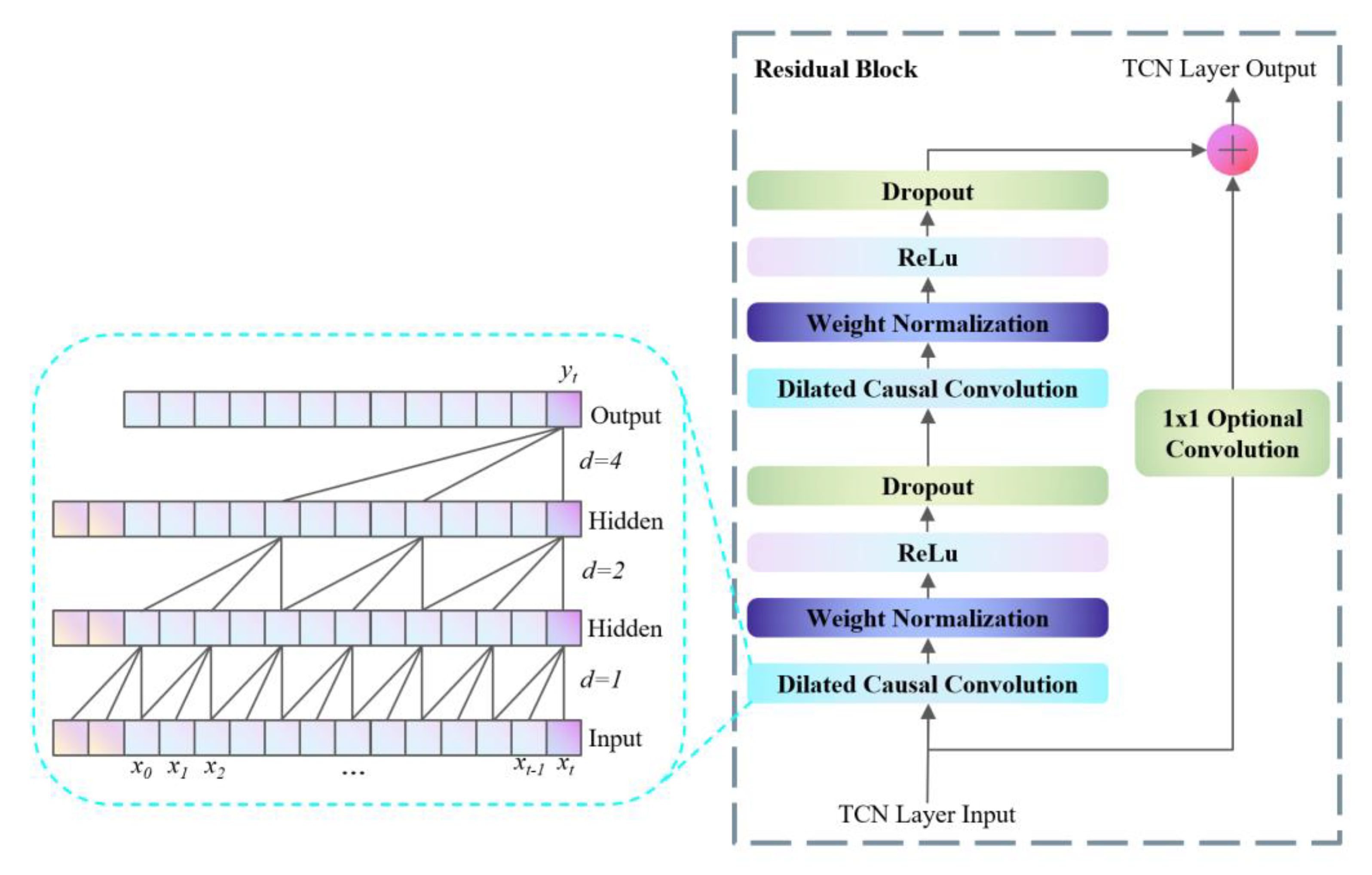
The architecture of the network is elaborately depicted in Figure 2, which illustrates that the TCN [48] primarily consists of three key components: causal convolution, dilated convolution, and residual connections. The design principle behind causal convolution is to ensure that the model’s predictions are based solely on past and present inputs, rather than future inputs, aligning with the temporal sequence’s natural causality. As demonstrated in the left portion of Figure 2, causal convolutions are structured such that the information for a given time point t incorporates data from preceding time points, thereby embedding a temporal hierarchy within the model layers. The effectiveness of causal convolution in feature extraction is constrained by the dimensions of its kernel, leading to the need for multiple linearly stacked layers to apprehend extensive dependencies. To address this limitation, TCNs employ an expanded convolution strategy, known as dilated convolution. Dilated convolutions, by design, require padding on either side of the input layer (left or right, depending on the convolution direction) commonly achieved through zero-padding. This approach allows for a broader receptive field without increasing the number of layers, thereby efficiently capturing wider temporal relationships without raising computational complexity or the number of parameters. The formal definition of dilated convolution is given by Equation (13):

$$F\left(s\right)=\left(x^{\ast }f\right)\left(s\right)={\displaystyle {\displaystyle \sum }_{i=0}^{k-1}}f\left(i\right)\cdot x_{s-d}\cdot i$$

(13)

where * denotes the convolution operation, $f$ represents the convolution kernel, $d$ represents the dilation factor, $k$ signifies the filter size, and $s$ indicates the sequence element for the dilated convolution. Typically, the dilation factor $d$ experiences an exponential increase in correlation with the network’s increasing depth. Augmenting both the dilation factor $d$ and the convolution kernel’s dimension $k$ results in an expanded receptive field for the TCN. Unlike standard convolutions, dilated convolutions sample the input at intervals, effectively expanding the receptive field with a controlled sampling rate determined by the dilation factor $d$.

As the number of layers in the network increases, it becomes essential to tackle challenges such as the vanishing gradient issue, necessitating the adoption of residual connections. Residual connections, particularly those utilizing $1\times 1$ convolution blocks, facilitate the cross-layer transmission of information, ensuring consistency between the inputs and outputs. The mathematical representation of these connections is presented below:

$$o=\mathit{Activation}\left(F\left(x\right)+x\right)$$

(14)

In this equation, $x$ denotes the input, $F\left(x\right)$ is the convolutional layer’s output, and $Activation\left( \right)$ signifies the ReLU activation function.

Displayed in the right section of Figure 2, the residual module encompasses a sequence starting with dilation causal convolution followed by weight normalization, application of ReLU for activation, and incorporation of a Dropout layer to prevent overfitting. This configuration is iterated across four stages, resulting in an eight-layer structure. Throughout this process, residual connections utilizing $1\times 1$ convolution blocks are employed to maintain consistent output dimensions.

2.5. Transformer

Transformers have achieved remarkable success in realms such as Natural Language Processing and image recognition, overcoming the limitations inherent in RNN and CNN-based forecasting models. CNNs often require many layers to achieve a significant receptive field, while RNNs rely on long time sequences for predictions. The self-attention mechanism of transformers addresses these issues by enabling direct access to sequence elements, thus facilitating a deeper exploration of the complex correlations within individual feature data. Moreover, their capacity for parallel processing significantly reduces training durations, allowing models to be trained on larger datasets compared to LSTM networks, enhancing their efficiency and applicability.

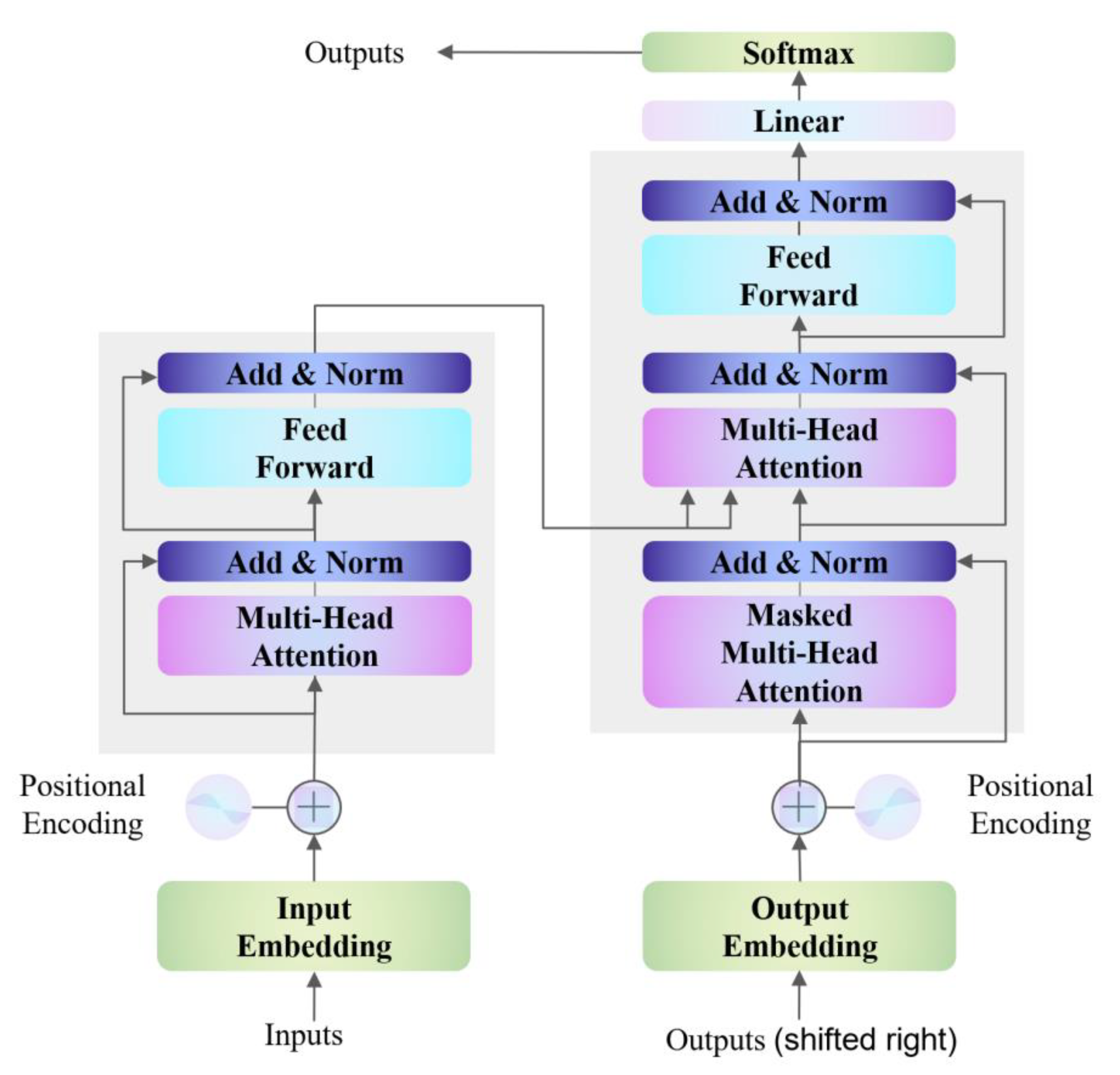
Figure 3 illustrates the intricate structure of the transformer network. The transformer architecture comprises two key elements: an encoder and a decoder [49]. The encoder is tasked with transforming the input into a rich, high-dimensional representation that encapsulates contextual nuances, whereas the decoder is dedicated to feature reconstruction [50]. Figure 3 delineates the comprehensive blueprint of the transformer model. Initial steps involve input embedding and position encoding before the data proceed to the encoder and decoder layers. Input embedding amalgamates various features into a unified representation, and position encoding ensures the retention of temporal attributes associated with each data point. The relevant mathematical formulation is provided as follows:

$$P_t^{\left(2i\right)}=\sin \left(w_{i}t\right),2i\le d$$

(15)

$$P_t^{\left(2i+1\right)}=\cos \left(w_{i}t\right),2i+1\le d$$

(16)

where $w_i=\frac{1}{{10000}^{2i^{\prime }d}}$; $t$ denotes the position index. The MHSA mechanism permits the model to concurrently compute linear transformations through various attention mechanisms, subsequently amalgamating diverse attentions to acquire a relatively more comprehensive feature information, thereby enhancing the efficacy of the self-attention layer. The MHSA mechanism emerges as a pivotal feature of the transformer, facilitating parallel processing of input data, a capability that sets it apart from sequential time sequence models like LSTM and TCN. Figure 3 provides a visual representation of the transformer’s architecture. Within the MHSA framework, the input vector $X$ is converted into $h$ distinct sets of query, key, and value matrices. The three distinct matrices known as Q (Query), K (Key), and V (Value) can be generated. The corresponding equations are depicted as follows:

$$\begin{gathered} Q_h=X{W}_h^Q \\ {K}_h=X{W}_h^K \\ {V}_h=X{W}_h^V \end{gathered}$$

(17)

where $Q_h$ denotes the query matrix, $K_h$ symbolizes the key matrix, and $V_h$ represents the value matrix, with $W_h^Q,W_h^K$ and $W_h^V$ being the adjustable parameters for the linear transformations. The MHSA divides the input into several independent feature spaces, facilitating the model’s ability to learn a broader spectrum of feature information [51]. The process continues with the application of scaled dot-product attention to generate a series of output vectors:

$$O_h=\mathrm{Attention}\left(Q_h,K_h,V_h\right)=\mathrm{softmax}\left(\frac{Q_{\mathrm{h}}{K}_{\mathrm{h}}^T}{\sqrt{d_K}}\right)V_h$$

(18)

Here, $O_h$ is the result of the scaled dot-product attention mechanism, with $\sqrt{d_K}$ acting as the scaling factor for the attention weights. The outputs, $O_h$, are subsequently concatenated and subjected to a linear projection to yield the final output.

$$MultiHeadSelfAttention \left(Q,K,V\right)=Concatenate\left(O_0,O_1,\dots ,O_h\right)W^O$$

(19)

where $W^O$ represents the learnable parameter of the MHSA mechanism, which is critical for encoding and aggregation info at each point for sequence.

3. Experiments and Discussion

3.1. Evaluation Indicators and Experimental Environment

Four frequently utilized indicators are employed to assess the efficacy of the experimental models: mean square error (MSE), mean absolute error (MAE), root-mean-square error (RMSE), and the R-squared (R²) score. The equations for these metrics are detailed as follows, where m represents the aggregate count of samples, ${\widehat{y}}_i$ denotes the forecasted values, $y_i$ corresponds to the observed values, and $\overline{y}$ is the average of $y_i$.

$$MSE=\frac{1}{m}{\displaystyle {\displaystyle \sum }_{i=1}^m}{(y_i-{\widehat{y}}_i)}^2$$

(20)

$$MAE=\frac{1}{m}{\displaystyle {\displaystyle \sum }_{i=1}^m}\left|\left(y_i-{\widehat{y}}_i\right)\right|$$

(21)

$$RMSE=\sqrt{\frac{1}{m}{\displaystyle {\displaystyle \sum }_{i=1}^m}{\left(y_i-{\widehat{y}}_i\right)}^2}$$

(22)

$$R^2=1-\frac{{{\displaystyle \sum }}_{i=1}^m{\left(y_i-{\widehat{y}}_i\right)}^2}{{{\displaystyle \sum }}_{i=1}^m{\left(y_i-\overline{y}\right)}^2}$$

(23)

The study’s experiments were performed using a system running on Windows 10 OS, utilizing the PyTorch framework alongside Python 3.9. The evaluations were conducted on hardware featuring an Intel Core CPU T7700, equipped with 32 GB of RAM and an NVIDIA Tesla M10 GPU. To ensure the fairness of the experiments, efforts were made to keep the parameters consistent across all models. The forecast periods considered are 12, 24, and 48, and the look-back periods are set at 24, 48, and 96. Batch size and epochs were standardized at 128 and 100, respectively, with Early Stop (patience = 3) and Dropout (dropout rate = 0.15) mechanisms implemented to counteract overfitting.

3.2. Datasets Description

To assess the performance of the proposed model, three unique datasets of wind speed, each from different geographical locations and with varied resolutions, were selected. The initial dataset originates from the National Renewable Energy Laboratory Wind Technology Center and is available to the public. The tower is located at 39°54′38.34″ N and 105°14′5.28″ W, with its base at an elevation of 1855 m above mean sea level. The data measurement height is 80 m, with a value resolution of 1 min. In this paper, 44,640 records from December 2020 are utilized, denoted as Dataset A. The second dataset originates from a wind farm in Wuwei City, Gansu Province, featuring a data measurement height of 70 m and a resolution of 10 min. This study utilizes 26,214 records from April to September 2019, referred to as Dataset B. The third dataset is sourced from a wind farm in Jiuquan City, Gansu Province, maintaining the same measurement height of 70 m but with a resolution of 15 min. It includes 58,368 records from January to December 2018, denoted as Dataset C. The forecast intervals are defined as 12, 24, and 48 steps, corresponding to actual prediction durations of 12, 24, and 48 minutes for Dataset A; 2, 4, and 8 hours for Dataset B; and 3, 6, and 12 hours for Dataset C, respectively. Each dataset was divided into three segments: 70% allocated for training, 10% for validation, and the remaining 20% for testing purposes. Figure 4 displays the fluctuation curves for data, while

Table 1. The statistical information.

Dataset	Resolution	Record	Min	Max	Mean	Std
Dataset A	1 min	44,640	0.27	24.73	4.23	4.04
Dataset B	10 min	26,214	0	24.93	4.76	3.49
Dataset C	15 min	58,368	0	28.44	5.98	3.58

shows a comprehensive overview of the datasets’ statistical characteristics, showcasing the unique statistical features of each dataset. Outliers were removed using the commonly employed quartile method, and missing values were addressed through cubic spline interpolation.

3.3. Experiment I

For the assessment of the developed model’s performance in terms of both accuracy and stability, we evaluated the suggested model against several benchmarks, including DBO-VMD-TCN, DBO-VMD-SVR, DBO-VMD-DLinear, DBO-VMD-PatchTST, DBO-VMD-Informer, and DBO-VMD-Transformer. The comparative analysis of errors across these models in three different datasets is detailed in

Table 2. The performance for Dataset A.

Step (Time)	Model	MSE	MAE	RMSE	R2
12 (12 m)	DBO-VMD-TCN	5.549	1.898	2.356	0.457
	DBO-VMD-SVR	0.845	0.553	0.919	0.937
	DBO-VMD-DLinear	1.414	0.796	1.189	0.862
	DBO-VMD-PatchTST	1.113	0.681	1.055	0.891
	DBO-VMD-Informer	0.354	0.403	0.595	0.965
	DBO-VMD-Transformer	0.353	0.379	0.594	0.965
	DBO-VMD-TCN-Transformer	0.160	0.269	0.400	0.984
24 (24 m)	DBO-VMD-TCN	5.715	1.966	2.391	0.441
	DBO-VMD-SVR	1.355	0.726	1.164	0.896
	DBO-VMD-DLinear	2.042	0.977	1.429	0.800
	DBO-VMD-PatchTST	1.686	0.848	1.298	0.835
	DBO-VMD-Informer	0.595	0.502	0.772	0.942
	DBO-VMD-Transformer	0.552	0.473	0.743	0.946
	DBO-VMD-TCN-Transformer	0.429	0.415	0.655	0.958
48 (48 m)	DBO-VMD-TCN	5.830	2.009	2.414	0.429
	DBO-VMD-SVR	2.224	0.973	1.496	0.825
	DBO-VMD-DLinear	2.683	1.138	1.638	0.737
	DBO-VMD-PatchTST	2.577	1.080	1.605	0.748
	DBO-VMD-Informer	0.801	0.592	0.895	0.922
	DBO-VMD-Transformer	0.741	0.559	0.861	0.927
	DBO-VMD-TCN-Transformer	0.630	0.523	0.794	0.938

Note: Values in bold indicate the best value.

,

Table 3. The performance for Dataset B.

Step (Time)	Model	MSE	MAE	RMSE	R2
12 (2 h)	DBO-VMD-TCN	4.629	1.559	2.151	0.571
	DBO-VMD-SVR	2.747	1.183	1.657	0.779
	DBO-VMD-DLinear	4.090	1.522	2.022	0.621
	DBO-VMD-PatchTST	3.241	1.295	1.800	0.700
	DBO-VMD-Informer	0.566	0.564	0.752	0.948
	DBO-VMD-Transformer	0.511	0.535	0.715	0.953
	DBO-VMD-TCN-Transformer	0.331	0.436	0.576	0.969
24 (4 h)	DBO-VMD-TCN	4.815	1.637	2.194	0.554
	DBO-VMD-SVR	4.558	1.549	2.135	0.612
	DBO-VMD-DLinear	5.768	1.825	2.402	0.466
	DBO-VMD-PatchTST	5.316	1.675	2.306	0.508
	DBO-VMD-Informer	1.109	0.791	1.053	0.897
	DBO-VMD-Transformer	0.993	0.732	0.997	0.908
	DBO-VMD-TCN-Transformer	0.723	0.640	0.850	0.933
48 (8 h)	DBO-VMD-TCN	4.782	1.677	2.187	0.558
	DBO-VMD-SVR	6.794	1.941	2.606	0.385
	DBO-VMD-DLinear	7.729	2.071	2.780	0.286
	DBO-VMD-PatchTST	7.317	2.083	2.705	0.324
	DBO-VMD-Informer	1.882	1.032	1.372	0.826
	DBO-VMD-Transformer	1.415	0.898	1.189	0.869
	DBO-VMD-TCN-Transformer	1.003	0.754	1.001	0.907

Note: Values in bold indicate the best value.

and

Table 4. The performance for Dataset C.

Step (Time)	Model	MSE	MAE	RMSE	R2
12 (3 h)	DBO-VMD-TCN	2.362	1.023	1.537	0.795
	DBO-VMD-SVR	3.809	1.364	1.951	0.714
	DBO-VMD-DLinear	4.249	1.472	2.061	0.632
	DBO-VMD-PatchTST	4.152	1.434	2.038	0.640
	DBO-VMD-Informer	0.516	0.519	0.718	0.955
	DBO-VMD-Transformer	0.390	0.451	0.625	0.966
	DBO-VMD-TCN-Transformer	0.214	0.342	0.463	0.981
24 (6 h)	DBO-VMD-TCN	3.355	1.226	1.832	0.709
	DBO-VMD-SVR	6.001	1.724	2.449	0.522
	DBO-VMD-DLinear	6.255	1.787	2.501	0.458
	DBO-VMD-PatchTST	6.182	1.780	2.486	0.465
	DBO-VMD-Informer	1.038	0.735	1.019	0.910
	DBO-VMD-Transformer	0.735	0.619	0.857	0.936
	DBO-VMD-TCN-Transformer	0.458	0.497	0.677	0.960
48 (12 h)	DBO-VMD-TCN	3.129	1.280	1.769	0.729
	DBO-VMD-SVR	8.591	2.078	2.931	0.261
	DBO-VMD-DLinear	8.943	2.164	2.990	0.225
	DBO-VMD-PatchTST	8.296	2.073	2.880	0.281
	DBO-VMD-Informer	1.784	0.969	1.336	0.845
	DBO-VMD-Transformer	1.166	0.777	1.080	0.899
	DBO-VMD-TCN-Transformer	0.895	0.665	0.946	0.922

Note: Values in bold indicate the best value.

, where the optimal outcomes are emphatically denoted in bold. Furthermore, Figure 5, Figure 6 and Figure 7 display forecast curves and columnar stacked charts, respectively, highlighting the forecasting capabilities of the six models over the three datasets.

The findings from Table 2, Table 3 and Table 4 reveal that the DBO-VMD-TCN-Transformer model outperforms other forecasting models in terms of prediction accuracy. The new hybrid model introduced in this study, which builds upon the TCN and transformer framework, demonstrates improved performance across various error metrics. Notably, this model demonstrates significant improvements in MAE, MSE, RMSE, and R², especially in the context of multi-step forecasting, when compared to the other model. For instance, in the 48-step prediction using the basic model, the TCN-Transformer exhibited the highest R², at 0.938, 0.907, and 0.922 for Datasets A, B, and C, respectively. In contrast, the R² values for the TCN networks in Datasets A, B, and C were 0.429, 0.558, and 0.729, respectively. In the 48-step forecasting using the SVR model, the TCN-Transformer exhibited the lowest MAE values for Datasets A, B, and C, recording 0.523, 0.754, and 0.665, respectively. In contrast, the MAE values for the SVR model were 0.973, 1.941, and 2.078 for Datasets A, B, and C, respectively.

The multi-step forecast curves, illustrated in Figure 5, Figure 6 and Figure 7, demonstrate that the model developed in this research outperforms alternative models in forecasting efficacy. By integrating the transformer model with the TCN, the approach achieves a superior fit to the predictive curve. The columnar stacked graphs in Figure 8 display the marked advantage of the combined forecasting model over other models in terms of overall performance. In Figure 8, the legends omit the common prefix part ‘DBO-VMD-’ of the models. This advantage is evident across four key metrics: MSE, MAE, RMSE, and R², each showing a trend of notable improvement. For example, during a 24-step prediction for Dataset B, the DBO-VMD-TCN model recorded MSE, MAE, and RMSE values of 4.815, 1.637, and 2.194, respectively. By contrast, the DBO-VMD-TCN-Transformer model dramatically improved upon these figures, posting values of 0.723, 0.640, and 0.850, respectively. This corresponds to performance enhancements of 85.0%, 60.9%, and 61.3% for these metrics, respectively. In the case of a 48-step forecast for Dataset C, the DBO-VMD-TCN model’s figures were 3.129, 1.280, and 1.769, while our model displayed superior figures of 0.895, 0.665, and 0.946, representing improvements of 71.4%, 48.0%, and 46.5%, respectively. Consequently, the hybrid approach introduced in this study achieves the most effective outcomes, leveraging the transformer’s robust forecasting capabilities alongside TCN’s enhanced feature extraction prowess. This combination effectively uncovers underlying correlations within extensive time series data, markedly elevating the hybrid model’s forecasting precision.

3.4. Experiment II

The predictive capabilities of the transformer, PatchTST, and informer were compared and analyzed under the same data decomposition method combined with the TCN.

Table 5. The performance of three models for Dataset A.

Step (Time)	Model	MSE	MAE	RMSE	R2
12 (12 m)	DBO-VMD-TCN-PatchTST	1.107	0.680	1.052	0.892
	DBO-VMD-TCN-Informer	0.178	0.275	0.422	0.983
	DBO-VMD-TCN-Transformer	0.160	0.269	0.400	0.984
24 (24 m)	DBO-VMD-TCN-PatchTST	1.679	0.863	1.296	0.836
	DBO-VMD-TCN-Informer	0.536	0.476	0.732	0.948
	DBO-VMD-TCN-Transformer	0.429	0.415	0.655	0.958
48 (48 m)	DBO-VMD-TCN-PatchTST	2.576	1.080	1.605	0.748
	DBO-VMD-TCN-Informer	0.741	0.583	0.861	0.927
	DBO-VMD-TCN-Transformer	0.630	0.523	0.794	0.938

Note: Values in bold indicate the best value.

,

Table 6. The performance of three models for Dataset B.

Step (Time)	Model	MSE	MAE	RMSE	R2
12 (2 h)	DBO-VMD-TCN-PatchTST	3.240	1.297	1.800	0.700
	DBO-VMD-TCN-Informer	0.410	0.488	0.640	0.962
	DBO-VMD-TCN-Transformer	0.331	0.436	0.576	0.969
24 (4 h)	DBO-VMD-TCN-PatchTST	5.271	1.671	2.296	0.512
	DBO-VMD-TCN-Informer	0.723	0.645	0.850	0.933
	DBO-VMD-TCN-Transformer	0.716	0.644	0.846	0.934
48 (8 h)	DBO-VMD-TCN-PatchTST	7.807	2.091	2.794	0.279
	DBO-VMD-TCN-Informer	1.308	0.861	1.144	0.879
	DBO-VMD-TCN-Transformer	1.003	0.754	1.001	0.907

Note: Values in bold indicate the best value.

and

Table 7. The performance of three models for Dataset C.

Step (Time)	Model	MSE	MAE	RMSE	R2
12 (3 h)	DBO-VMD-TCN-PatchTST	4.133	1.431	2.033	0.642
	DBO-VMD-TCN-Informer	0.234	0.356	0.484	0.980
	DBO-VMD-TCN-Transformer	0.214	0.342	0.463	0.981
24 (6 h)	DBO-VMD-TCN-PatchTST	6.281	1.793	2.506	0.456
	DBO-VMD-TCN-Informer	0.483	0.509	0.695	0.958
	DBO-VMD-TCN-Transformer	0.458	0.497	0.677	0.960
48 (12 h)	DBO-VMD-TCN-PatchTST	8.865	2.164	2.977	0.231
	DBO-VMD-TCN-Informer	1.065	0.739	1.032	0.908
	DBO-VMD-TCN-Transformer	0.895	0.665	0.946	0.922

Note: Values in bold indicate the best value.

provide a detailed comparative analysis of the error metrics for these models across three distinct datasets, with the optimal values highlighted in bold. Furthermore, Figure 9 illustrates the 3D histograms, emphasizing the prediction abilities of the three models on the three datasets.

As shown in Table 5, Table 6 and Table 7, the transformer model outperforms the informer and PatchTST models in multi-step prediction across distinct datasets. Regarding the MSE, MAE, and RMSE indicators, where lower values are preferable, the transformer model shows a marked decrease in these values when compared to the PatchTST and informer models. This is corroborated by the outcomes of multi-step forecasting shown in Table 5, Table 6 and Table 7. For instance, during a 48-step prediction in Dataset B, the MAE values recorded were 2.091, 0.861, and 0.754, respectively. These findings highlight a notably better performance in the transformer model while indicating a somewhat inferior result in the informer model. Therefore, the transformer model reveals a considerable capacity for enhancement. This not only boosts the overall accuracy of the model but also guarantees a more precise reflection of the actual figures.

From the 3D histograms in Figure 9, it is evident that the transformer model yields superior outcomes compared to the PatchTST and informer models across Datasets A, B, and C. In the figure, the legends omit the common prefix part ‘DBO-VMD-TCN’ of the models. For instance, in a 24-step prediction for three datasets, the transformer model shows a notable enhancement over the PatchTST model, with average increases of 36.8% in R² metrics. The transformer model demonstrated significant improvements over the PatchTST model, with similar trends observed in Datasets A, B, and C. Moreover, during the 48-step prediction phase for three datasets, the transformer model registers an average enhancement of 15.1% across three metrics over informer, with average increases of 22.3%, 12.3%, and 10.6% in MSE, MAE, RMSE, respectively.

3.5. Experiment III

To assess the effectiveness of the DBO-VMD method in decomposing wind-speed series data, comparisons were made with scenarios without VMD, with VMD, and with VMD optimized by PSO. For the optimized VMD, the penalty factor was chosen within the range of [500, 3000], and the value of K was set between 3 and 10, inclusive of integers only. For the non-optimized VMD, the K value was empirically set to 7. Both DBO and PSO optimization algorithms were configured with two variables, ten individuals, and a maximum of thirty iterations. Subsequently, DBO was utilized to optimize the VMD parameters. Figure 10 illustrates that the optimal number of IMFs was determined to be 8. The time domain of the modal components obtained through DBO-VMD decomposition is shown in the left portion of Figure 10. It is evident from the right portion of Figure 10 that each mode is distinct in the frequency distribution of the modal components, effectively preventing the issue of mode mixing.

Table 8. The performance of different optimization algorithms.

Step (Time)	Model	MSE	MAE	RMSE	R2
12 (3 h)	TCN-Transformer	3.858	1.395	1.964	0.666
	VMD-TCN-Transformer	0.608	0.555	0.780	0.947
	PSO-VMD-TCN-Transformer	0.466	0.491	0.683	0.960
	DBO-VMD-TCN-Transformer	0.214	0.342	0.463	0.981
24 (6 h)	TCN-Transformer	5.895	1.737	2.428	0.489
	VMD-TCN-Transformer	0.789	0.637	0.888	0.932
	PSO-VMD-TCN-Transformer	0.735	0.619	0.857	0.936
	DBO-VMD-TCN-Transformer	0.458	0.497	0.677	0.960
48 (12 h)	TCN-Transformer	8.224	2.076	2.868	0.287
	VMD-TCN-Transformer	1.797	0.969	1.340	0.844
	PSO-VMD-TCN-Transformer	1.373	0.844	1.172	0.881
	DBO-VMD-TCN-Transformer	0.895	0.665	0.946	0.922

Note: Values in bold indicate the best value.

’s analysis shows that employing the VMD method results in substantial performance improvements across four metrics compared to without VMD. For instance, in a 24-step forecast, the MSE, MAE, RMSE, and R² values for the VMD method were 0.789, 0.637, 0.888, and 0.932, respectively. In contrast, the values for these metrics without using the VMD method were significantly less favorable. These findings demonstrate that VMD is an effective data decomposition model for enhancing predictive accuracy. A comprehensive analysis of Table 8 reveals that the DBO-VMD-TCN-Transformer model achieved outstanding evaluation metrics in three types of multi-step forecasts. Through comparative assessments, the forecasting outcomes based on the DBO-VMD and PSO-VMD hybrid models demonstrated an improvement of 34.8%, 21.2%, 19.3%, and 4.7% across the metrics of MSE, MAE, RMSE, and R², respectively. These critical indicators highlight the superior performance of the combined model employing DBO for optimizing VMD parameters over the model using PSO optimization for VMD.

Figure 11 presents radar charts that compare the performance indicators for VMD both with and without the decomposition methods, alongside the application of different optimization algorithms. In the legend, ‘Transformer’ is abbreviated as ‘Tr’. The Key indicators of MSE, MAE, and RMSE are recorded with preferable outcomes indicated by lower scores. It is evident from the chart that the DBO-VMD-TCN-Transformer model secures minimal values across these performance measures. Regarding the 1-R² metric, which when nearer to 0 denotes greater precision, the WSO-VMD-TCN-Transformer model is shown to be the closest to this optimal benchmark. This finding highlights the efficacy of the DBO-VMD approach in enhancing the accuracy and fit of wind-speed predictions.

3.6. Diebold Mariano Test

The DM test is comparable to conducting a t-test, focusing on comparing the average losses produced by two distinct predictive models to determine if they are statistically identical. When dealing with time series data that show autocorrelation, the DM test adeptly adjusts its estimation of the standard deviation for the difference in losses, taking autocorrelation into account. This capability renders the DM test especially effective for evaluating forecasting models tailored to time series data. The foundational premise, or the null hypothesis (H0), posited by the test is the absence of any significant discrepancy in the predictive accuracies of the two models being compared. Nonetheless, as detailed in

Table 9. The DM test results.

Dataset	Step	12		24		48
	Model	DM	P	DM	P	DM	P
Dataset A	DBO-VMD-TCN	−29.75	1.01 × 10−193	−42.23	0	−61.45	0
	DBO-VMD-SVR	−15.56	7.23 × 10−46	−18.52	3.16 × 10−85	−28.96	1.83 × 10−223
	DBO-VMD-DLinear	−14.90	3.54 × 10−50	−23.31	5.53 × 10−120	−35.48	2.45 × 10−275
	DBO-VMD-PatchTST	−14.04	9.11 × 10−45	−19.31	5.11 × 10−83	−31.64	2.08 × 10−219
	DBO-VMD-Informer	−17.71	4.24 × 10−70	−18.14	1.67 × 10−73	−21.08	1.26 × 10−98
	DBO-VMD-Transformer	−14.59	3.52 × 10−48	−15.06	3.13 × 10−51	−15.38	2.23 × 10−53
Dataset B	DBO-VMD-TCN	−21.09	1.99 × 10−98	−30.77	4.41 × 10−207	−45.42	0
	DBO-VMD-SVR	−17.06	2.73 × 10−65	−22.17	5.26 × 10−95	−35.36	2.68 × 10−257
	DBO-VMD-DLinear	−16.84	1.77 × 10−63	−23.06	2.07 × 10−117	−36.77	4.12 × 10−295
	DBO-VMD-PatchTST	−16.85	1.45 × 10−63	−21.01	7.77 × 10−98	−33.85	1.51 × 10−250
	DBO-VMD-Informer	−19.16	1.39 × 10−81	−22.70	8.34 × 10−114	−40.42	0
	DBO-VMD-Transformer	−17.55	9.05 × 10−69	−13.05	6.90 × 10−39	−33.02	1.45 × 10−238
Dataset C	DBO-VMD-TCN	−17.51	1.63 × 10−68	−39.64	0	−56.04	0
	DBO-VMD-SVR	−19.86	5.37 × 10−93	−27.46	8.37 × 10−206	−48.17	0
	DBO-VMD-DLinear	−20.97	1.86 × 10−97	−29.82	5.33 × 10−195	−46.81	0
	DBO-VMD-PatchTST	−20.74	2.12 × 10−95	−31.67	1.51 × 10−219	−47.06	0
	DBO-VMD-Informer	−19.30	6.80 × 10−83	−28.23	5.23 × 10−175	−49.06	0
	DBO-VMD-Transformer	−17.90	1.45 × 10−71	−22.00	3.72 × 10−107	−34.68	3.41 × 10−263

, differences in the predictive accuracies of the models are observed at the 5% significance level. Table 9 demonstrates that H0 is rejected for every comparison model, suggesting a distinct difference in the predictive capabilities of the DBO-VMD-TCN-Transformer model compared to its counterparts. The data in Table 9, which shows all p-values below 0.05 and all DM values as negative, support the conclusion that the combined prediction model introduced in this research significantly outperforms the benchmark models in terms of forecasting accuracy.

3.7. Discussion

Previous research results indicate that, compared to other models, the proposed model exhibits significant advantages across three datasets and various step lengths. This is attributed to its reliance on a hybrid model capable of handling high-resolution wind-speed fluctuation information. The superiority of the DBO-VMD-TCN-Transformer model can be summarized as follows:

VMD Preprocessing: As demonstrated by the experiments in Section 3.5, there is a noticeable difference in the forecasting results with and without VMD preprocessing. Optimization through DBO further enhances the effectiveness of VMD preprocessing. VMD preprocessing improves the non-stationarity of the original wind speeds. therefore, all experimental comparisons in this paper are based on VMD-preprocessed data.

TCN Module: As observed in Section 3.3, standalone TCN predictions perform the worst. However, hybrid models that combine TCNs with transformer-like structures outperform those without TCN integration. The TCN module excels in extracting temporal features from high-resolution wind speeds, thereby enhancing the performance of the hybrid forecasting models.

Transformer Module: As demonstrated in Section 3.4, hybrid models equipped with transformer modules yield better forecasting results than non-transformer hybrid models. Furthermore, transformer-based hybrid models surpass those integrating informer and PatchTST models. The transformer module effectively captures complex dependencies between input data and forecast outputs, achieving optimal predictive performance.

4. Conclusions

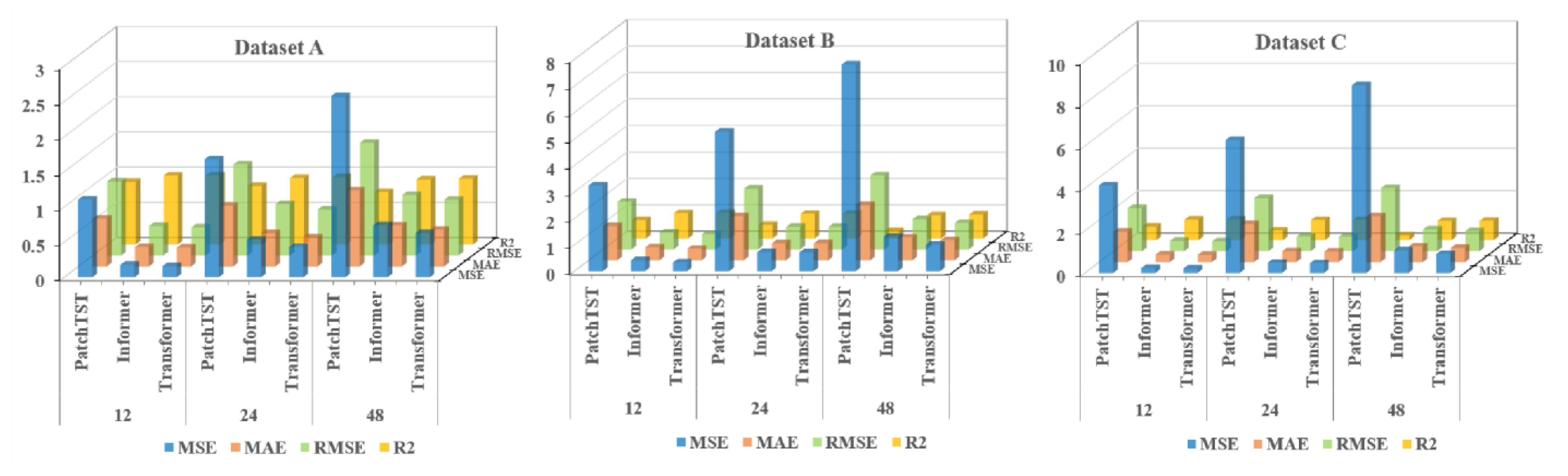
Addressing the need for enhanced accuracy in wind-speed forecasting and the scarcity of research on wind-speed short-term prediction utilizing the transformer architecture, this study introduces a hybrid wind-speed prediction model that integrates the transformer model, VMD, and TCNs. This innovative model aims to leverage the strengths of each component to enhance accuracy and efficiency in predicting wind speeds across various time horizons. By integrating the transformer’s ability to handle complex dependencies with the accuracy of VMD for wind-speed decomposing and the efficiency of TCNs for temporal analysis, this proposed model seeks to fill the gaps in current short-term wind-speed forecasting methodologies and extend the application of transformer-based models to a wider range of forecasting scenarios. The efficacy of the introduced model was validated and assessed using three real-world datasets. Experiments conducted with these datasets revealed that (1) compared to six benchmark models, the proposed model exhibits superior performance, showing an average improvement of 54.2% in MSE, MAE, and RMSE performance, and a 52.1% increase in R² performance. (2) The transformer model demonstrates enhanced capabilities in short-term forecasting compared to the PatchTST and informer models. On average, its performance in the MSE, MAE, and RMSE metrics improved by 40.2%, while the R² score increased by 20.8%. (3) The DBO-VMD strategy has proven effective in enhancing the accuracy and consistency of wind-speed forecasting results. Compared to models without VMD, the DBO-VMD-TCN-Transformer hybrid model shows an average performance improvement of 78.5% in MSE, MAE, and RMSE metrics, and a 50.0% increase in the R² score. (4) The DM test indicates that the model exhibits statistically significant improvements over other baseline models at the 5% significance level.

Challenges include the incomplete optimization of hyperparameters and a deficit in error evaluation. Future research will delve into comprehensive studies on transformer-based hybrid models, the automation of hyperparameter optimization, and detailed error correction, with the aim of enhancing the precision of wind-speed predictions.

References

1. Majidi Nezhad, M.; Neshat, M.; Piras, G.; Astiaso Garcia, D. Sites Exploring Prioritisation of Offshore Wind Energy Potential and Mapping for Wind Farms Installation: Iranian Islands Case Studies. Renew. Sustain. Energy Rev. 2022, 168, 112791. [Google Scholar] [CrossRef]
2. GWEC. Global Wind Report 2023-Global Wind Energy Council. Available online: https://gwec.net/globalwindreport2023/ (accessed on 1 November 2023).
3. Lv, S.-X.; Wang, L. Multivariate Wind Speed Forecasting Based on Multi-Objective Feature Selection Approach and Hybrid Deep Learning Model. Energy 2023, 263, 126100. [Google Scholar] [CrossRef]
4. Liu, H.; Chen, C. Data Processing Strategies in Wind Energy Forecasting Models and Applications: A Comprehensive Review. Appl. Energy 2019, 249, 392–408. [Google Scholar] [CrossRef]
5. Meka, R.; Alaeddini, A.; Bhaganagar, K. A Robust Deep Learning Framework for Short-Term Wind Power Forecast of a Full-Scale Wind Farm Using Atmospheric Variables. Energy 2021, 221, 119759. [Google Scholar] [CrossRef]
6. Heng, J.; Hong, Y.; Hu, J.; Wang, S. Probabilistic and Deterministic Wind Speed Forecasting Based on Non-Parametric Approaches and Wind Characteristics Information. Appl. Energy 2022, 306, 118029. [Google Scholar] [CrossRef]
7. Sri Preethaa, K.R.; Muthuramalingam, A.; Natarajan, Y.; Wadhwa, G.; Ali, A.A.Y. A Comprehensive Review on Machine Learning Techniques for Forecasting Wind Flow Pattern. Sustainability 2023, 15, 12914. [Google Scholar] [CrossRef]
8. Yang, W.; Tian, Z.; Hao, Y. A Novel Ensemble Model Based on Artificial Intelligence and Mixed-Frequency Techniques for Wind Speed Forecasting. Energy Convers. Manag. 2022, 252, 115086. [Google Scholar] [CrossRef]
9. Zhao, J.; Guo, Z.; Guo, Y.; Lin, W.; Zhu, W. A Self-Organizing Forecast of Day-Ahead Wind Speed: Selective Ensemble Strategy Based on Numerical Weather Predictions. Energy 2021, 218, 119509. [Google Scholar] [CrossRef]
10. Hu, J.; Heng, J.; Wen, J.; Zhao, W. Deterministic and Probabilistic Wind Speed Forecasting with De-Noising-Reconstruction Strategy and Quantile Regression Based Algorithm. Renew. Energy 2020, 162, 1208–1226. [Google Scholar] [CrossRef]
11. Erdem, E.; Shi, J. ARMA Based Approaches for Forecasting the Tuple of Wind Speed and Direction. Appl. Energy 2011, 88, 1405–1414. [Google Scholar] [CrossRef]
12. Aasim; Singh, S.N.; Mohapatra, A. Repeated Wavelet Transform Based ARIMA Model for Very Short-Term Wind Speed Forecasting. Renew. Energy 2019, 136, 758–768. [Google Scholar] [CrossRef]
13. Dowell, J.; Pinson, P. Very-Short-Term Probabilistic Wind Power Forecasts by Sparse Vector Autoregression. IEEE Trans. Smart Grid 2015, 7, 763–770. [Google Scholar] [CrossRef]
14. Jung, J.; Broadwater, R.P. Current Status and Future Advances for Wind Speed and Power Forecasting. Renew. Sustain. Energy Rev. 2014, 31, 762–777. [Google Scholar] [CrossRef]
15. Song, J.; Wang, J.; Lu, H. A Novel Combined Model Based on Advanced Optimization Algorithm for Short-Term Wind Speed Forecasting. Appl. Energy 2018, 215, 643–658. [Google Scholar] [CrossRef]
16. Zhang, S.; Zhu, C.; Guo, X. A Novel Combined Model Based on Hybrid Data Decomposition, MSWOA and ENN for Short-Term Wind Speed Forecasting. Int. J. Comput. Sci. 2023, 50, 22. [Google Scholar]
17. He, X.; Nie, Y.; Guo, H.; Wang, J. Research on a Novel Combination System on the Basis of Deep Learning and Swarm Intelligence Optimization Algorithm for Wind Speed Forecasting. IEEE Access 2020, 8, 51482–51499. [Google Scholar] [CrossRef]
18. Liu, D.; Niu, D.; Wang, H.; Fan, L. Short-Term Wind Speed Forecasting Using Wavelet Transform and Support Vector Machines Optimized by Genetic Algorithm. Renew. Energy 2014, 62, 592–597. [Google Scholar] [CrossRef]
19. Guo, X.; Zhu, C.; Hao, J.; Zhang, S. Multi-Step Wind Speed Prediction Based on an Improved Multi-Objective Seagull Optimization Algorithm and a Multi-Kernel Extreme Learning Machine. Appl. Intell. 2022, 53, 16445–16472. [Google Scholar] [CrossRef]
20. Zhao, X.; Wang, C.; Su, J.; Wang, J. Research and Application Based on the Swarm Intelligence Algorithm and Artificial Intelligence for Wind Farm Decision System. Renew. Energy 2019, 134, 681–697. [Google Scholar] [CrossRef]
21. Wang, H.Z.; Wang, G.B.; Li, G.Q.; Peng, J.C.; Liu, Y.T. Deep Belief Network Based Deterministic and Probabilistic Wind Speed Forecasting Approach. Appl. Energy 2016, 182, 80–93. [Google Scholar] [CrossRef]
22. Harbola, S.; Coors, V. One Dimensional Convolutional Neural Network Architectures for Wind Prediction. Energy Convers. Manag. 2019, 195, 70–75. [Google Scholar] [CrossRef]
23. Memarzadeh, G.; Keynia, F. A New Short-Term Wind Speed Forecasting Method Based on Fine-Tuned LSTM Neural Network and Optimal Input Sets. Energy Convers. Manag. 2020, 213, 112824. [Google Scholar] [CrossRef]
24. Wu, J.; Li, N.; Zhao, Y.; Wang, J. Usage of Correlation Analysis and Hypothesis Test in Optimizing the Gated Recurrent Unit Network for Wind Speed Forecasting. Energy 2022, 242, 122960. [Google Scholar] [CrossRef]
25. Zou, Z.; Wang, J.; E, N.; Zhang, C.; Wang, Z.; Jiang, E. Short-Term Power Load Forecasting: An Integrated Approach Utilizing Variational Mode Decomposition and TCN–BiGRU. Energies 2023, 16, 6625. [Google Scholar] [CrossRef]
26. Franceschi, J.-Y.; Dieuleveut, A.; Jaggi, M. Unsupervised Scalable Representation Learning for Multivariate Time Series. In Proceedings of the Advances in Neural Information Processing Systems, Vancouver, BC, Canada, 8–14 December 2019; Wallach, H., Larochelle, H., Beygelzimer, A., Alché-Buc, F., d’Fox, E., Garnett, R., Eds.; Curran Associates, Inc.: New York, NY, USA, 2019; Volume 32. [Google Scholar]
27. Zhang, Y.; Zhang, L.; Sun, D.; Jin, K.; Gu, Y. Short-Term Wind Power Forecasting Based on VMD and a Hybrid SSA-TCN-BiGRU Network. Appl. Sci. 2023, 13, 9888. [Google Scholar] [CrossRef]
28. Liu, X.; Zhou, J.; Qian, H. Short-Term Wind Power Forecasting by Stacked Recurrent Neural Networks with Parametric Sine Activation Function. Electr. Power Syst. Res. 2021, 192, 107011. [Google Scholar] [CrossRef]
29. Zhang, Z.; Wang, J.; Wei, D.; Luo, T.; Xia, Y. A Novel Ensemble System for Short-Term Wind Speed Forecasting Based on Two-Stage Attention-Based Recurrent Neural Network. Renew. Energy 2023, 204, 11–23. [Google Scholar] [CrossRef]
30. Neshat, M.; Nezhad, M.M.; Abbasnejad, E.; Mirjalili, S.; Tjernberg, L.B.; Astiaso Garcia, D.; Alexander, B.; Wagner, M. A Deep Learning-Based Evolutionary Model for Short-Term Wind Speed Forecasting: A Case Study of the Lillgrund Offshore Wind Farm. Energy Convers. Manag. 2021, 236, 114002. [Google Scholar] [CrossRef]
31. Chen, M.; Peng, H.; Fu, J.; Ling, H. AutoFormer: Searching Transformers for Visual Recognition. In Proceedings of the IEEE/CVF International Conference on Computer Vision (ICCV), Montreal, BC, Canada, 11–17 October 2021; pp. 12270–12280. [Google Scholar]
32. Wu, H.; Meng, K.; Fan, D.; Zhang, Z.; Liu, Q. Multistep Short-Term Wind Speed Forecasting Using Transformer. Energy 2022, 261, 125231. [Google Scholar] [CrossRef]
33. Zhou, H.; Zhang, S.; Peng, J.; Zhang, S.; Li, J.; Xiong, H.; Zhang, W. Informer: Beyond Efficient Transformer for Long Sequence Time-Series Forecasting. Proc. AAAI Conf. Artif. Intell. 2021, 35, 11106–11115. [Google Scholar] [CrossRef]
34. Yang, K.; Shi, F. Medium- and Long-Term Load Forecasting for Power Plants Based on Causal Inference and Informer. Appl. Sci. 2023, 13, 7696. [Google Scholar] [CrossRef]
35. Bommidi, B.S.; Teeparthi, K.; Kosana, V. Hybrid Wind Speed Forecasting Using ICEEMDAN and Transformer Model with Novel Loss Function. Energy 2023, 265, 126383. [Google Scholar] [CrossRef]
36. Huang, S.; Zhang, J.; He, Y.; Fu, X.; Fan, L.; Yao, G.; Wen, Y. Short-Term Load Forecasting Based on the CEEMDAN-Sample Entropy-BPNN-Transformer. Energies 2022, 15, 3659. [Google Scholar] [CrossRef]
37. Wang, Y.; Xu, H.; Song, M.; Zhang, F.; Li, Y.; Zhou, S.; Zhang, L. A Convolutional Transformer-Based Truncated Gaussian Density Network with Data Denoising for Wind Speed Forecasting. Appl. Energy 2023, 333, 120601. [Google Scholar] [CrossRef]
38. Zeng, A.; Chen, M.; Zhang, L.; Xu, Q. Are Transformers Effective for Time Series Forecasting? In Proceedings of the AAAI Conference on Artificial Intelligence arXiv, Washington, DC, USA, 17 August 2022; Volume 37. pp. 11121–11128. [Google Scholar] [CrossRef]
39. Nie, Y.; Nguyen, N.H.; Sinthong, P.; Kalagnanam, J. A Time Series Is Worth 64 Words: Long-Term Forecasting with Transformers. arXiv 2023, arXiv:2211.14730. [Google Scholar]
40. Ye, L.; Li, Y.; Pei, M.; Zhao, Y.; Li, Z.; Lu, P. A Novel Integrated Method for Short-Term Wind Power Forecasting Based on Fluctuation Clustering and History Matching. Appl. Energy 2022, 327, 120131. [Google Scholar] [CrossRef]
41. Li, J.; Song, Z.; Wang, X.; Wang, Y.; Jia, Y. A Novel Offshore Wind Farm Typhoon Wind Speed Prediction Model Based on PSO–Bi-LSTM Improved by VMD. Energy 2022, 251, 123848. [Google Scholar] [CrossRef]
42. Wu, B.; Wang, L.; Zeng, Y.-R. Interpretable Wind Speed Prediction with Multivariate Time Series and Temporal Fusion Transformers. Energy 2022, 252, 123990. [Google Scholar] [CrossRef]
43. Geng, G.; He, Y.; Zhang, J.; Qin, T.; Yang, B. Short-Term Power Load Forecasting Based on PSO-Optimized VMD-TCN-Attention Mechanism. Energies 2023, 16, 4616. [Google Scholar] [CrossRef]
44. Zhang, C.; Ma, H.; Hua, L.; Sun, W.; Nazir, M.S.; Peng, T. An Evolutionary Deep Learning Model Based on TVFEMD, Improved Sine Cosine Algorithm, CNN and BiLSTM for Wind Speed Prediction. Energy 2022, 254, 124250. [Google Scholar] [CrossRef]
45. Altan, A.; Karasu, S.; Zio, E. A New Hybrid Model for Wind Speed Forecasting Combining Long Short-Term Memory Neural Network, Decomposition Methods and Grey Wolf Optimizer. Appl. Soft Comput. 2021, 100, 106996. [Google Scholar] [CrossRef]
46. Liu, H.; Yang, R.; Wang, T.; Zhang, L. A Hybrid Neural Network Model for Short-Term Wind Speed Forecasting Based on Decomposition, Multi-Learner Ensemble, and Adaptive Multiple Error Corrections. Renew. Energy 2021, 165, 573–594. [Google Scholar] [CrossRef]
47. Xue, J.; Shen, B. Dung Beetle Optimizer: A New Meta-Heuristic Algorithm for Global Optimization. J. Supercomput. 2023, 79, 7305–7336. [Google Scholar] [CrossRef]
48. Bai, S.; Kolter, J.Z.; Koltun, V. An Empirical Evaluation of Generic Convolutional and Recurrent Networks for Sequence Modeling. arXiv 2018, arXiv:1803.01271. [Google Scholar]
49. Vaswani, A.; Shazeer, N.; Parmar, N.; Uszkoreit, J.; Jones, L.; Gomez, A.N.; Kaiser, Ł.; Polosukhin, I. Attention Is All You Need. In Proceedings of the Advances in Neural Information Processing Systems, Long Beach, CA, USA, 4–9 December 2017; Curran Associates, Inc.: New York, NY, USA, 2017; Volume 30. [Google Scholar]
50. He, K.; Chen, X.; Xie, S.; Li, Y.; Dollár, P.; Girshick, R. Masked Autoencoders Are Scalable Vision Learners. In Proceedings of the IEEE/CVF Conference on Computer Vision and Pattern Recognition, New Orleans, LA, USA, 18–24 June 2022; pp. 16000–16009. [Google Scholar]
51. Li, S.; Jin, X.; Xuan, Y.; Zhou, X.; Chen, W.; Wang, Y.-X.; Yan, X. Enhancing the Locality and Breaking the Memory Bottleneck of Transformer on Time Series Forecasting. In Proceedings of the Advances in Neural Information Processing Systems, Vancouver, BC, Canada, 8–14 December; Curran Associates, Inc.: New York, NY, USA, 2019; Volume 32. [Google Scholar]
Figure 1. Flowchart of the developed model.
Energies 17 01996 g001
Figure 2. The architecture of TCN.
Energies 17 01996 g002
Figure 3. The transformer architecture.
Energies 17 01996 g003
Figure 4. The original wind speeds.
Energies 17 01996 g004
Figure 5. The forecasting results of Dataset A.
Energies 17 01996 g005
Figure 6. The forecasting results of Dataset B.
Energies 17 01996 g006
Figure 7. The forecasting results of Dataset C.
Energies 17 01996 g007
Figure 8. Columnar stacked chart of various models.
Energies 17 01996 g008
Figure 9. The 3D histograms.
Energies 17 01996 g009
Figure 10. The IMFs and spectrum of DBO-VMD decomposition.
Energies 17 01996 g010
Figure 11. The radar chart.
Energies 17 01996 g011