Qualification and Quantification of Porosity at the Top of the Fuel Pins in Metallic Fuels Using Image Processing

Abstract

Approximately 130,000 metal fuel pins were irradiated in the Experimental Breeder Reactor II (EBR-II) during its 30 years of operation to develop and characterize existing and prospective fuels. For many of the metal fuel irradiation experiments, neutron radiography imaging was performed to characterize fuel behavior, such as fuel axial expansion. While several fuel expansion results obtained from neutron radiography imaging have been published, the analysis of neutron radiography for the purpose of describing statistical properties of porous matter formed on top of the fuel pins, also referred to as fluff in previous publications, is significantly less represented in the literature with just a single paper so far. This study aims to validate and augment results reported in previous publications using automated image processing. The paper describes the statistical properties of the porous matter in terms of nine parameters derived from radiography images and correlates those parameters with such fuel properties as composition, expansion, temperature, and burnup. The reported results are based on 1097 fuel pins of eight different fuel compositions. For three major fuel types, U-10Zr, U-8Pu-10Zr, and U-19Pu-10Zr, a clear negative correlation is found between the Pu content and five parameters describing the amount of porous matter generated. The parameters describing granularity properties, however, showed either negative correlation or nonlinear dependency from fuel composition. The parameters describing the amount showed a positive correlation with fuel axial expansion, while granularity parameters showed a negative correlation with axial expansion. The dependency on cladding temperature was found to be weak. A positive correlation is demonstrated for volume parameters and fuel burnup. In general, reported results confirm and validate findings published in previous studies using a much larger number of pins and automated processing techniques, which easily lend themselves to reproducibility, thus avoiding subjective bias.

1. Introduction

In its 30-year history, the Experimental Breeder Reactor II (EBR-II)—a key irradiation facility for metal fuel development—underwent a number of transformations, starting as a demonstration test bed for a closed loop fuel cycle and was instrumental in supporting the Integral Fast Reactor (IFR) program [1]. Fuel technology is a key aspect of sodium-cooled fast reactor (SFR) systems, affecting reactor safety, reactor operations, fuel reprocessing technology, and overall system economics [2,3,4,5,6,7,8,9,10]. Two major types of fuel were extensively studied and qualified as driver fuels for SFRs in the United States (U.S.) and around the world: mixed oxide fuel (MOX) and metallic fuel.

One advantage of metallic fuels is their higher thermal conductivity (liquid metal), which enables the fuel to operate at lower temperatures with reduced stored energy. In addition, metallic fuels have a more favorable neutron economy, higher fuel densities, and easier fabrication and reprocessing processes [1]. The advantage of metallic fuels is their high burnup limit in comparison with MOX fuels, with U-19Pu-10Zr achieving a 110 gigawatt-days/metric ton of heavy metal (GWD/MTHM) if operated on a three-burn cycle, while MOX fuel will peak at 65 GWD/MTHM. In this paper, we consider U-10Zr, U-8Pu-10Zr, and U-19Pu-10Zr fuel compositions within the irradiated EBR-II fuel pins.

Regardless of the type of fuel, the timeline for qualification of advanced nuclear fuel design is inordinately prolonged by the costs and inefficiencies in generating, analyzing, and modeling nuclear experimental data. For example, a single nuclear fuel or materials experiment may contain relatively few experimental specimens yet cost as much as USD 5 to USD 10 M each, require more than five years per cycle, and require four to five experiment cycles to obtain satisfactory qualification data (i.e., 20–25 years in total) [3]. Crawford et al. [1] outlined the steps for qualification, indicating that it takes 20–25 years for complete development and licensing for metallic fuels. The research effort presented in this paper is directed towards shortening the development time and accelerating the licensing process for fuel, as this research’s success applied to a given fuel performance characteristic is transferable to other key fuel characteristics and to other fuel types as knowledge and proficiency increase.

The existence of a porous structure (previously referred to as fluff) at the top of metallic fuel pins used in Experimental Breeder Reactor II (EBR-II) has been well documented, and its properties were recently analyzed [11,12]. The post-irradiation examination using scanning electron microscopy, X-ray spectroscopy, and electron probe microanalyzer [11] revealed that the structure on top of the fuel pins contains the elements of ternary fuel (U, Pu, Zr), which are observed as regions of different porosity and oxidation [11]. The single pin examined in [11] was subjected to a moderate overpower. However, the observed three-microstructure redistribution behavior [13] for fuel regions is in line with the previous literature. Moreover, rare earth precipitates were found in the porous structure. An important finding of the microstructural analysis was that the porous regions contained fuel with as-prefabricated elemental compositions in addition to expected fission products [11]. The porosity of the different fuel regions was thoroughly investigated, and it was found that lower porosity was present near the cladding and larger pores within the inner pin regions. The porosity analysis is very important as it serves as a stepping stone to the analysis performed in this study. This, however, because of the nature of microstructural examination, can only be performed on a small number of pins or images.

In this study, statistical analysis of the porous structure was conducted to study the dependence between its formation and operating conditions, such as fuel burnup, inner cladding temperature, and the dependence between the structure’s height/extent and fuel swelling [12]. The study examined 670 pins of different fuel compositions and subjected them to different burnups and cladding temperatures. In the previous study [12], the only parameter of the porous structure at the top of the pins that was investigated was its height, which was manually measured on neutron radiography images. A definite dependency between the porosity’s height and fuel composition has been demonstrated with a clear indication of a Pu suppressive effect on porosity formation. However, the suppressive effect seemed to saturate at mid-range Pu concentrations. It was found that a significant positive correlation between the height of the porous structure and fuel burnup exists for all types of fuel composition, with the U-10Zr fuel demonstrating the highest positive correlation. A significant negative correlation was found between the height of the porosity and peak inner cladding temperature. Finally, the dependency between the fuel’s axial swelling and porosity was found to be weak and required further investigation.

This paper extends the work presented in [12] by applying image processing methods to a larger number of pins and enhancing the uncertainty quantification for the formation of the porous structure. Applying automatic methods of analysis has several advantages, such as eliminating subjectivity in measurements, faster processing of large volumes of imaging data, rigorous quantification of uncertainty in parameter estimation, and the ability to evaluate parameters that are hard to quantify with visual analysis. All these may help to better understand and model the behavior of this particular feature of metallic fuel rods.

2. Data and Materials

2.1. Neutron Radiography Images

To study porosity at the top of fuel pins, 185 EBR-II neutron radiography images were used. Each image contained six fuel pins with different fuel compositions. The total number of processed pins was 1097, with 661 unique pins since many pins were used repeatedly in different experiments to study fuel’s properties under different burnup conditions. The pins’ distributions according to fuel composition are shown in

Table 1. Number of pins according to fuel composition.

Fuel Composition	Number of Pins
U-10Zr	529
U-19Pu-10Zr	293
U-19Pu-14Zr	10
U-19Pu-6Zr	9
U-22Pu-10Zr	25
U-26Pu-10Zr	24
U-3Pu-10Zr	20
U-8Pu-10Zr	187

.

The largest number of pins is U-10Zr pins, followed by U-19Pu-10Zr and U-8Pu-10Zr as the most common fuel compositions. The other fuel compositions are rather exotic, and the number of pins is about 10 times smaller. For the pins investigated in this paper, four different types of cladding were used during irradiation experiments: 316SS, D9, HT9, and HT9M. The median length of manufactured unirradiated pins investigated in this paper was 34.31 cm, with five U-19Pu-10Zr pins having a much shorter median initial length of 28.04 cm.

The irradiated metallic fuel pins discussed in this paper were radiographed using dysprosium foil detectors most sensitive to thermal neutrons [14]. The activated foils were then used to transfer images to film. The thermal neutrons provide images with better contrast at the expense of a shallower penetration of the fuel. For this paper, the higher contrast images are indispensable and were favored over epithermal neutron imaging. A detailed description of neutral radiography imaging can be found in [14]. Images on film were subsequently digitized using a scanner to obtain images in a JPEG format. These JPEG images were used as the original images for the image processing algorithms presented in this paper.

The general pipeline of image processing used in this paper is shown in Figure 1. After reading an image into RAM, the original image is converted into a grayscale image. The next step is to adjust the image intensity or contrast so that the signal-to-noise ratio can be improved. After this contrast adjustment, image binarization is performed to remove gray areas and perform image segmentation. Since binarization is a nonlinear operation, it performs all-or-nothing filtering, setting gray areas either as white pixels or black pixels. Using a binary image from a previous step, a connectivity algorithm is applied to detect connected areas of white pixels. Since most white pixels will represent the fuel, the connectivity operation effectively segments the image into the fuel part and the fluff part. Further, each foreground region of the image is labeled to attribute it to a pin.

Smaller foreground regions are eliminated by setting them to the background, thus removing objects that are not part of the fuel pins. Having labeled the image regions, the algorithm groups the labeled objects by pin. For each pin, its fluff parameters are calculated, and statistical analysis is performed. These image-processing steps are further described in more detail in the following sections. Codes designed to characterize fuel growth were developed using MATLAB’s Image Processing Toolbox R2017b.

2.2. Image Formats and Conversion

The original JPEG images of neutron radiography were acquired with 150 dpi resolution using a 35 mm focal length camera, and on average, have the size of 4300 by 10,000 pixels with a color depth of 24 bits. The JPEG image format uses a compression algorithm to store the image; however, it is decompressed while being loaded into RAM and takes the same amount of RAM as lossless formats such as TIFF. Since a very limited number of images was available in TIFF format, all raw images used in this project were either originally in JPEG format or were converted to JPEG from TIFF. The original JPEG images use RGB color coding, which requires three bytes to represent each pixel. Since the neutron radiographs have no meaningful color information, the RGB images prior to processing were converted into grayscale images. Since each channel in the RGB image has 256 shades, the RGB image was converted into grayscale by taking the weighted sum of the R, G, and B values. Specifically, for this paper, the conversion formula is:

$$\mathrm{G}\mathrm{r}\mathrm{a}\mathrm{y}=0.2989\times \mathrm{R}+0.5870\times \mathrm{G}+0.1140\times \mathrm{B}.$$

(1)

The triplet of weights (0.2989, 0.5870, 0.1140) used in the conversion formula comes from BT.601-7 [15] recommendations developed by the International Telecommunication Union. Since all three channels in the grayscale image are set to the same level, only one byte is necessary to store each pixel, thus reducing RAM requirements by a factor of three.

3. Image Processing

3.1. Intensity Enhancement and Binarization

The first step in determining the characteristics of the most porous part of irradiated fuel pins is to isolate it from the less porous solid part, which can be performed through different types of image thresholding. A typical grayscale radiography image is shown in Figure 2.

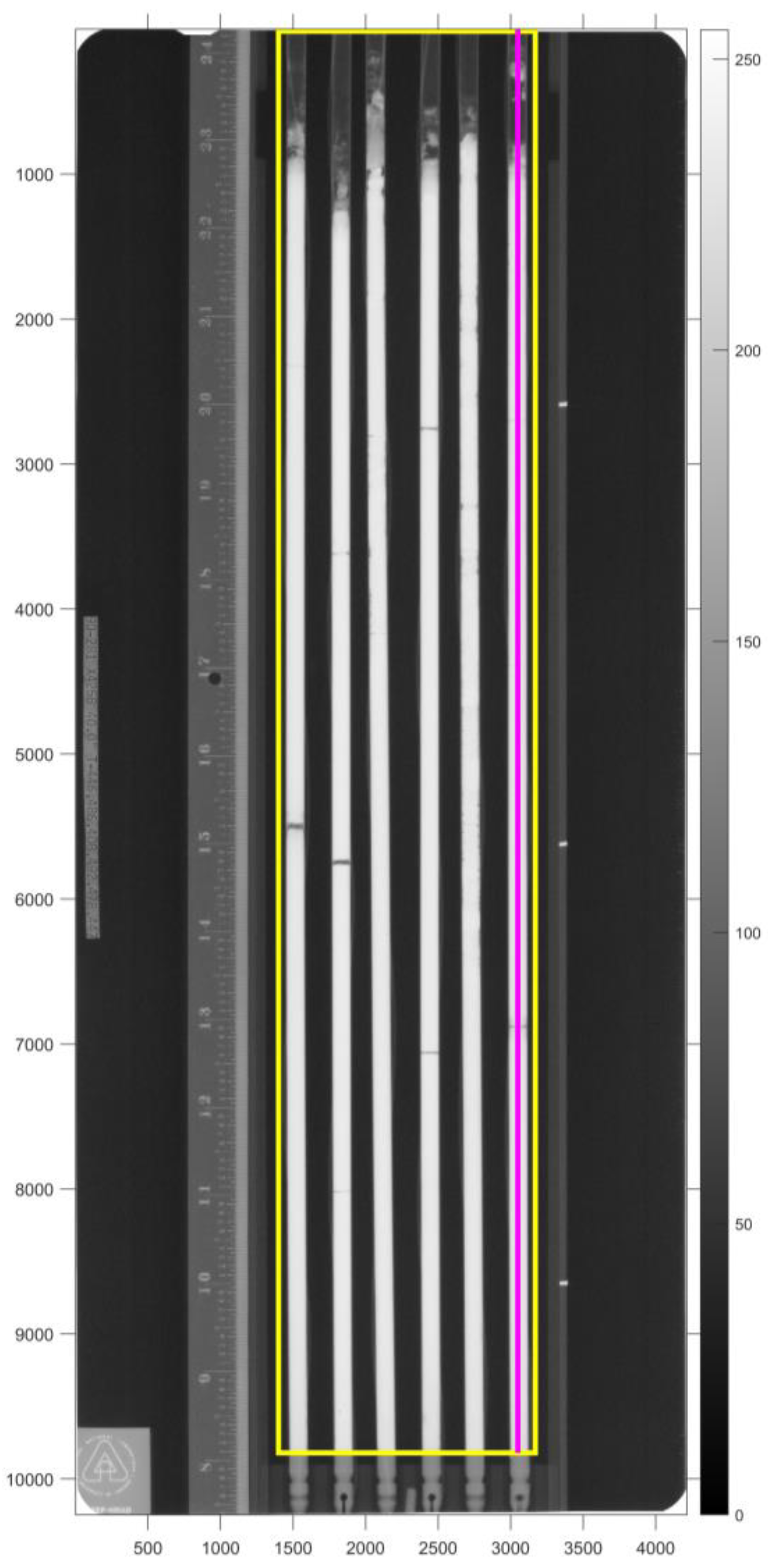
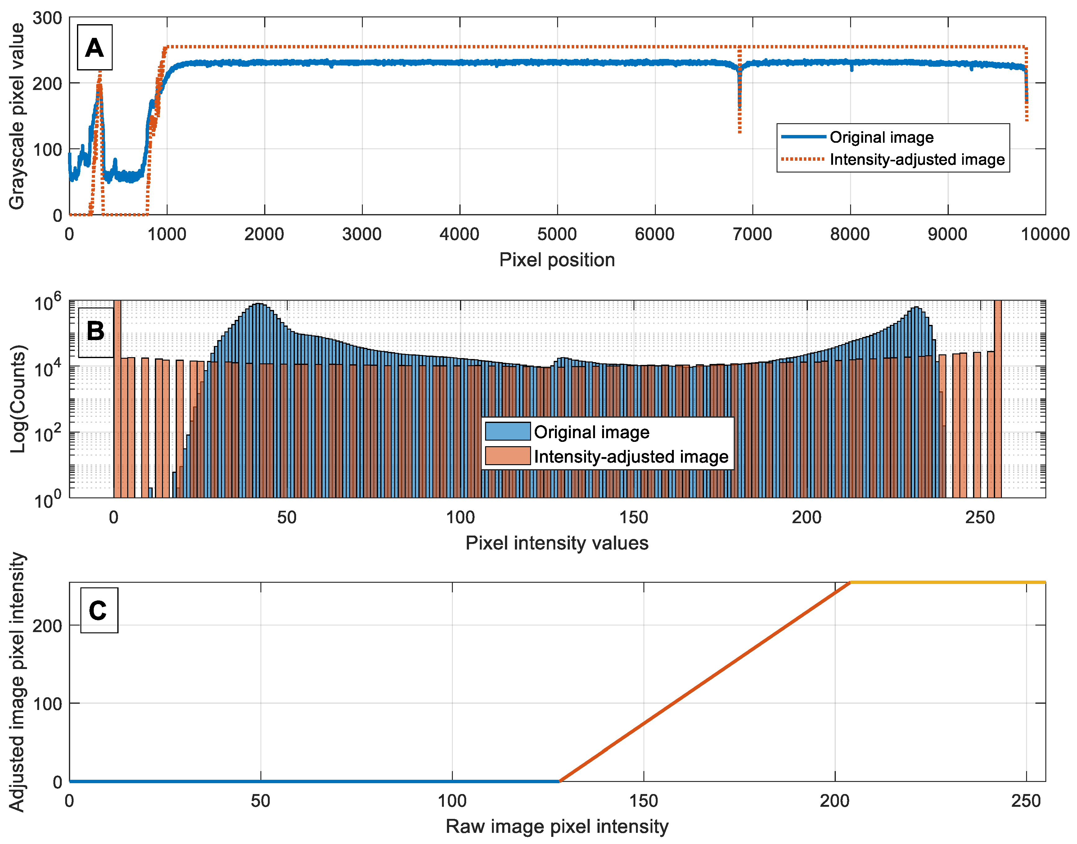
It can be seen that all fuel pins in this image have a varying degree of visible porous structure formed at the top. Also, four out of six pins in Figure 2 have visible cracks, as well as other radiation-induced defects such as bending. The pixel’s intensity for grayscale images ranges from 0 (black) to 255 (white), and the intensity bar on the right shows the intensity scale of the image. The x- and y-axes on the image show the image dimensions in pixels. In addition to the images of the pins, the original image also contains a dark background as well as some auxiliary information such as a ruler, a plaque with pin numbers, and a logo in the bottom left corner. The ruler and pin numbers are relevant information; however, pixel-wise, they represent noise. The first step in image processing is to isolate regions of porosity on top of the fuel pins from the solid part of the pins. A very valuable tool for image analysis is an image histogram, which represents the distribution of pixels according to their gray-level values. Based on the histogram, the pixels’ intensity can be adjusted, and image contrast can be improved. The top panel A of Figure 3 shows the image cross-cut along the magenta line in Figure 1 for the raw and intensity-adjusted images. The pixel’s positions are plotted from left to right, with position zero corresponding to the top of the image in Figure 2. Most pixels in the raw image have intensities between 200 and 250, and they correspond to the solid part of the fuel pin.

The dip in intensity close to the pixel’s position 6865 in panel A corresponds to a crack in the fuel pin. The pixels in the positions between 0 and 1000 in panel A of Figure 3 correspond to the porous section of the fuel pin. The first step of analysis is to segregate the solid section, which accounts for the pins’ irradiation swelling, from the porous section, which is of interest for this study. This segregation process is called image segmentation and is usually accomplished using a preset threshold for pixel intensity values such that pixels with intensities higher than the threshold are counted as one object while pixels with lower values are counted as a different object. While it is obvious from panel A of Figure 3 that setting the segmentation threshold at around an intensity value of 200 will separate the solid section from the porous one, the exact value of such a threshold is debatable. The segmentation thresholds are usually set by analyzing the image histogram [16]. If an image contains pixels of different intensities belonging to different objects, those objects will be manifested as different modes on the image histogram. The histogram of the original image in the yellow rectangle cutout in Figure 2 is shown in panel B of Figure 3. Notice the log scale of the y-axis for the histogram plot. The histogram of the original image clearly has three modes: the high-intensity pixels with a mode value of around 230, the low-intensity pixels with a mode around 42, and the middle-intensity pixels with a smaller mode of around 130. The low-intensity mode corresponds to dark background pixels; the high-intensity mode is the bright pixels representing the solid part of the fuel pin, while the middle range mode is the gray pixels, the majority of which are the porous matter on top of the fuel pin. The edges between dark background pixels and bright pin’s pixels are also represented by gray pixels. The goal of the segmentation is to isolate the pins from the porosity on top.

Based on the histogram of the original image, the threshold selection is problematic as there is no clear cutoff pixel value that would separate the solid part of the fuel pin from its porous part. Applying automated threshold selection algorithms such as the Otsu method [17] to the histogram of the original image results in the threshold value of 134, which places the threshold squarely in the middle of the histogram. To facilitate the segmentation, the process of intensity adjustment is applied to the raw image, which attempts to increase the separability of different objects by mapping pixels’ intensity values to new values such that the new intensity values are further apart. The middle panel B in Figure 3 shows the effect of applying linear intensity adjustment to the part of the image shown in a yellow rectangle in Figure 1. The bottom panel C of Figure 3 shows the intensity-mapping function used to produce an intensity-adjusted histogram in panel B. For this study, a linear piece-wise intensity-mapping function was used, which requires selecting two cutoff values. The first is the low-intensity threshold below which the pixels’ intensity is set to 0 (black); the second one is a high-intensity threshold above which the pixels’ intensity is set to 1 (white). The pixels’ intensities between these two thresholds are mapped linearly into new values, as shown in panel C of Figure 2. For this study, the low-intensity threshold was set to 128, which is around the middle-intensity mode shown on the original image histogram of panel B in Figure 3.

The threshold was selected based on the desire to preserve pixels corresponding to the porosity as well as edge pixels from the pins. The threshold’s value was set after analyzing numerous histograms of raw images. The high-intensity threshold was set to 204, which corresponds to the flat portion of the image cross-cut shown in panel A of Figure 3. The intensity adjustment can be considered as a “soft” thresholding as there is a range of intensities that are neither mapped into zero nor into 255. The histogram of the intensity-adjusted image is shown in panel B of Figure 3. It can be seen that the intensity-adjusted histogram is stretched to the extreme values of intensity values, and it clearly has two modes: the lower mode placed at an intensity value of 0 and the upper mode placed at an intensity value of 255. This histogram stretching improves the image signal-to-noise ratio and allows the next step in image processing to be performed: image binarization. Image binarization is contrast enhancement taken to the extreme. Instead of using “soft” thresholding when some gray-level pixels are mapped with a linear function, image binarization applies hard thresholding to intensity values, values below the binarization threshold are set to zero, and values above the threshold are set to 255. The binarization threshold can be selected using the histogram of the intensity-adjusted image obtained in the previous step. Based on the analysis of intensity-adjusted histograms of radiographic images used in this study, the binarization threshold was set to 218 and applied across all images. An alternative approach is to apply multiple thresholds to the original image without the additional step of intensity adjustment. This process is known as image quantization. The effects of applying intensity adjustment, binarization, and quantization to a radiography image are shown in Figure 4.

As can be seen from the two leftmost images in Figure 4, the gray areas on the top of the fuel pins representing low-density and disintegrated fuel were blacked out by setting the corresponding pixels to zero, while the solid areas of the fuel pins were set to one. The rightmost image in Figure 4 represents the effect of the application of two thresholds selected by the Otsu method. The two thresholds selected by the Otsu method had intensity values of 73 and 164. These thresholds parse image histograms into three sections: below 73, between 73 and 164, and above 164. Pixels with intensity values less or equal to 73 are assigned label 1, pixels between 73 and 164 are assigned label 2, while pixels with intensity values higher than 164 are assigned label 3. Having a labeled image allows the image to be displayed with different shades of gray, as shown in the rightmost image in Figure 4. While the multi-thresholding segregates pins from the background and the fluff, it also creates problems, such as relegating many areas to the fluff label. The white color on the rightmost image in Figure 4 is assigned to pins and has label 3; label 2 pixels are shown with a gray color, while the background pixels assigned label 1 are shown in black. It can be seen that along with fluff regions, the gray-colored label 2 is assigned to some auxiliary parts of the image, such as the ruler on the left. Some of those gray areas can be eliminated by cropping the image; however, the gray pixels on top have some features that will be very difficult to segregate from the fluff, such, for example, as wiring running along the pins and visible on top of the pins. For this reason, the two-step approach of contrast adjustment and subsequent binarization was adopted in this paper.

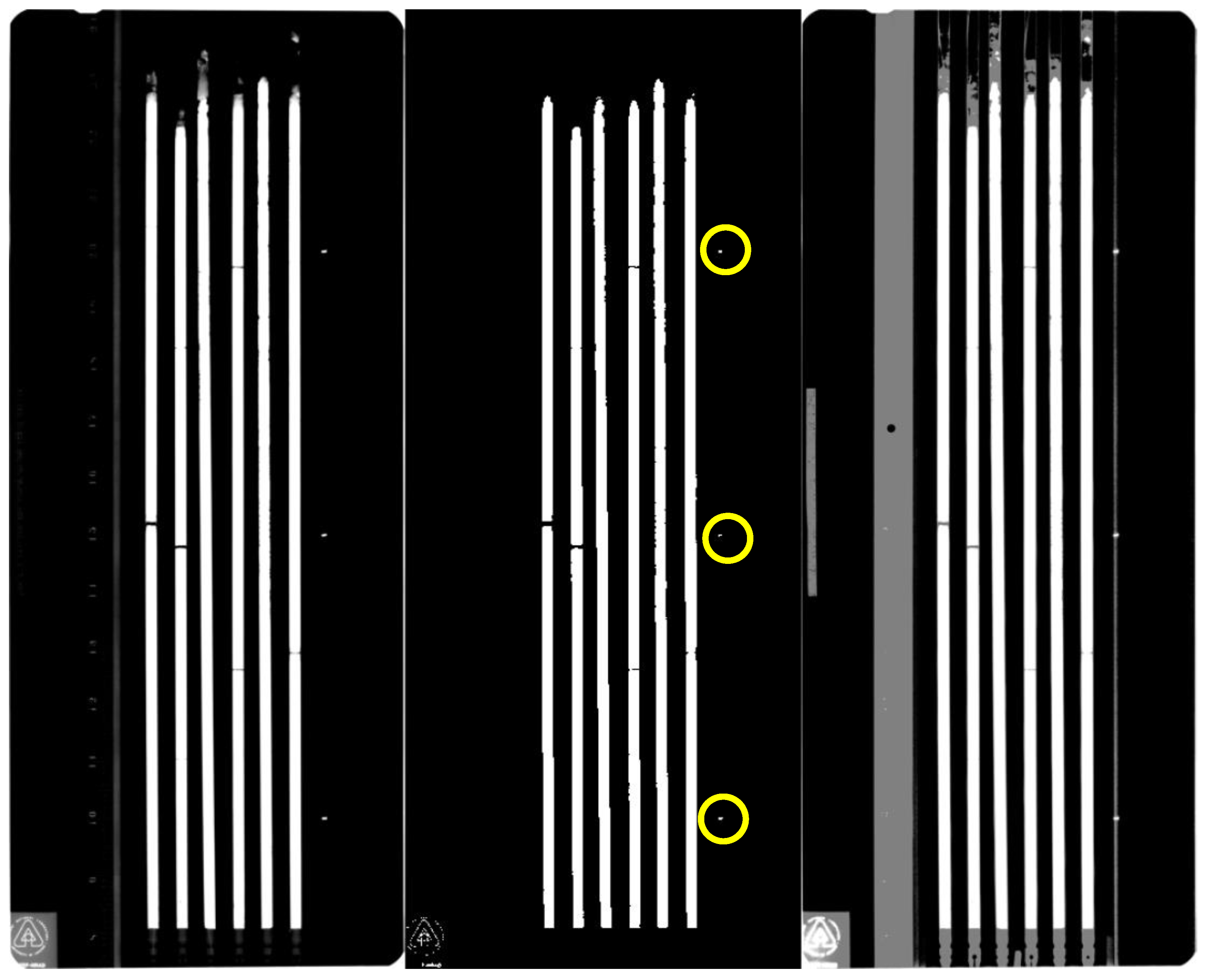
While image binarization is an effective tool for eliminating gray areas in the image, it cannot deal with small, isolated areas of high intensities, as shown in the center image in Figure 4, where small bright areas are circled in yellow. Since those areas have pixel values higher than the binarization threshold, they will survive the operation of binarization, and their removal requires an additional step based on the size of the areas rather than pixel values. The pixels set to high intensities in these images are called foreground or object pixels, while the pixels set to low intensities are called background pixels. Finding connected areas of foreground and background pixels is the subject of connectivity analysis.

The connectivity analysis is used in this paper to achieve two goals: (1) identify and remove small, connected areas of high-intensity pixels from the image and (2) identify parts of the image representing the same fuel pin. The connectivity analysis algorithms used in this paper are described in [18,19].

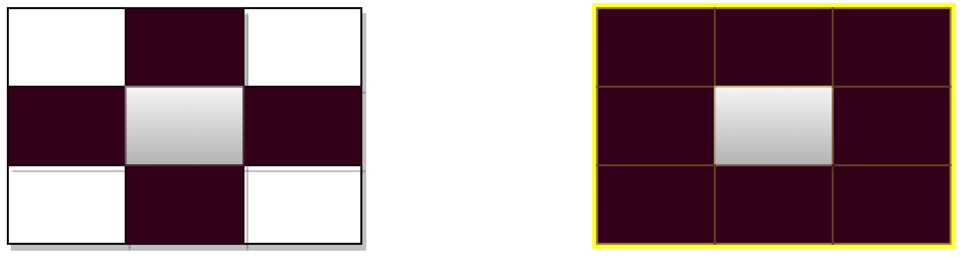
In image connectivity analysis, two major pixel neighborhood connectivity diagrams are used: 4-connectivity diagrams and 8-connectivity diagrams, as illustrated in Figure 5. For 8-connectivity analysis, the pixel is counted as connected to its neighboring pixels if the pixel is a foreground pixel and touches its neighboring foreground pixels along the edges or on the corners. If any neighboring pixel is a background pixel, it is considered disconnected from the pixel of interest.

The application of connectivity analysis to radiography images is described in our previous paper [20]. The output of connectivity analysis is regions of pixels labeled as belonging to a single object. The value of each region labeling for the purpose of removing small areas of bright pixels is that after each labeled region is found, the total area of the region can be calculated, and the regions with areas smaller than a preselected threshold can be set as the background. The threshold was selected by analyzing the histogram of area sizes and set to 20 K pixels (i.e., all regions with a total area less than or equal to 20 K pixels were set as the background). The histogram of the area sizes demonstrated a bimodal nature, with one mode representing large regions and the other mode representing small regions. The 20 K threshold was in the valley separating those two modes and was selected as a cutoff value. It should be pointed out that the algorithm is not sensitive to increasing the values of the area threshold as the area of the pins is significantly larger than the area of the “fluff”. The results of applying area thresholding to the binarized image are shown in Figure 6. As can be seen, the small high-intensity regions shown with yellow circles have been removed from the binary image, while the resulting image represents only the solid parts of the six fuel pins. In summary, image thresholding involves a selection of four thresholds: low and high thresholds for intensity adjustment, binarization threshold, and area-size threshold or morphological opening threshold. The first two thresholds are selected based on the analysis of the raw image histograms, as shown in Figure 3; the binarization threshold is selected based on the analysis of the histogram of the intensity-adjusted image, as described above. Finally, the threshold to perform morphological opening is selected based on the analysis of the histogram of area sizes. After extracting the fuel pins from the image, we can now isolate individual pins using the same connectivity analysis and region labeling previously applied to the binarized image. The goal of this analysis is to isolate separate pins from each other and identify regions belonging to the same pin. A detailed description of this step is given in [20].

3.2. Pins Localization

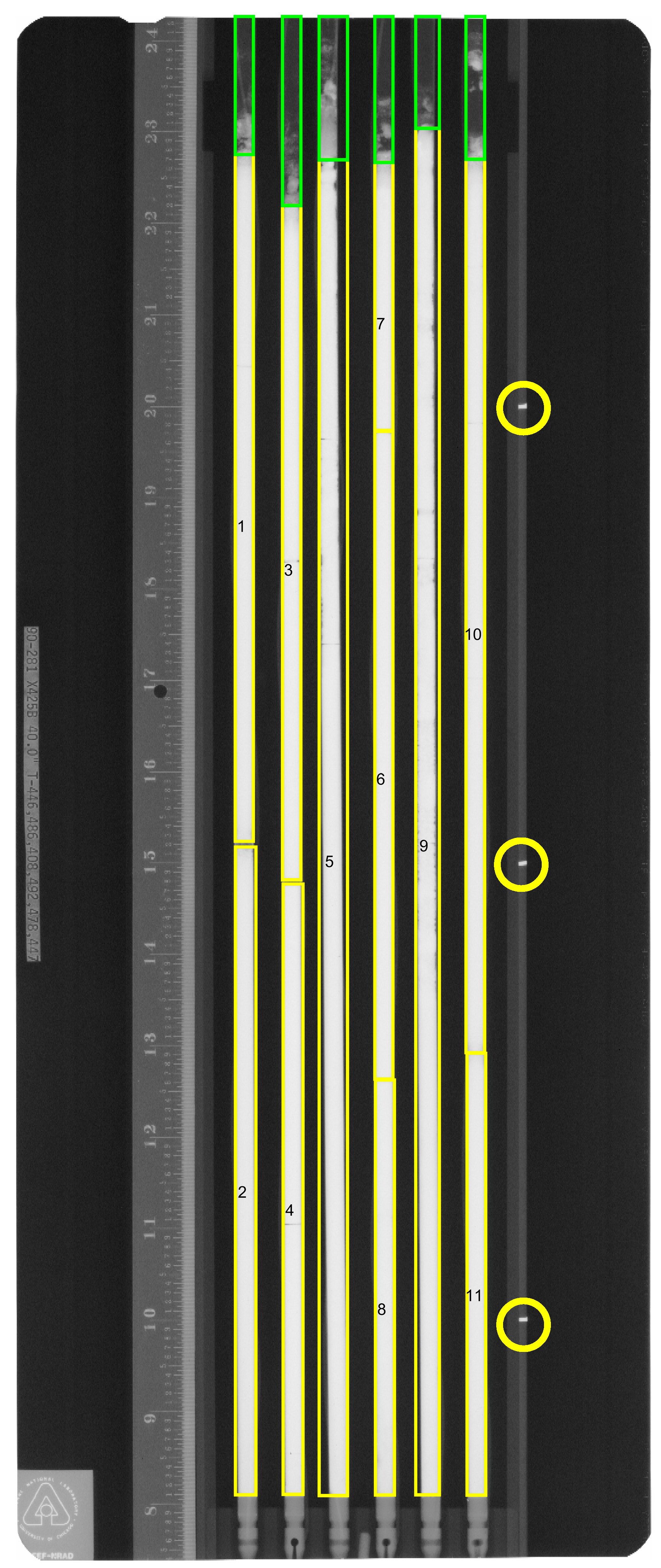
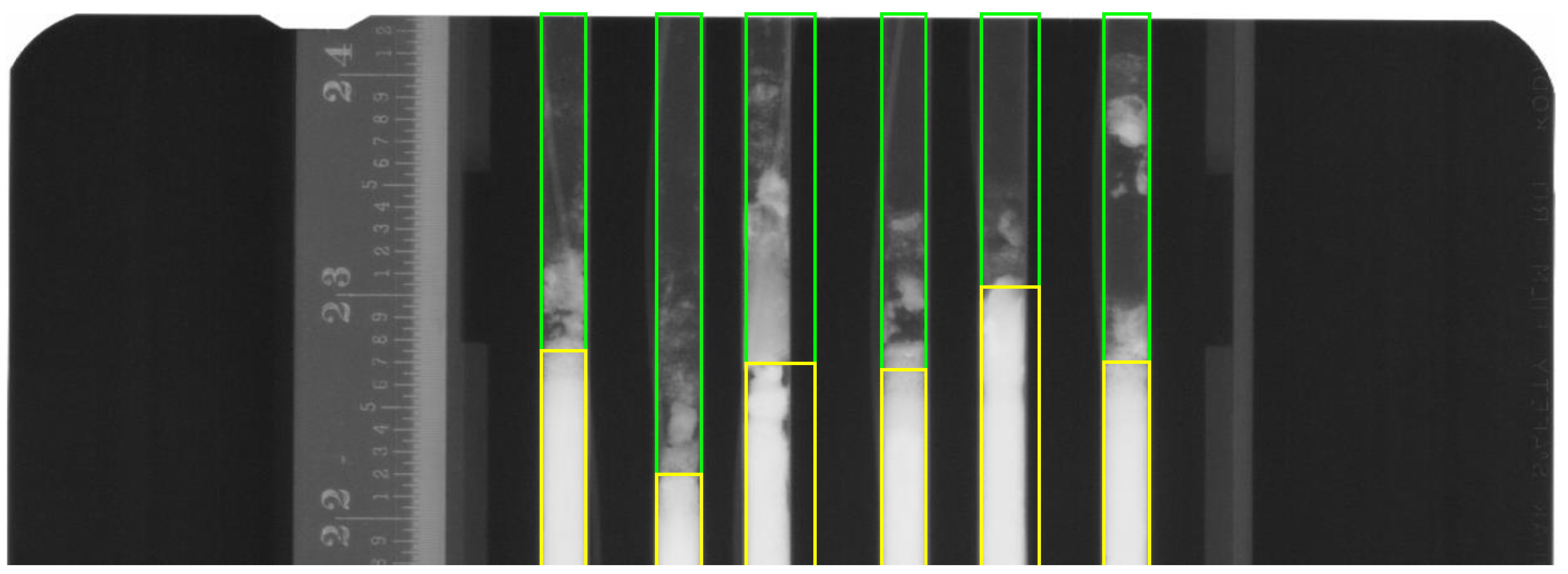
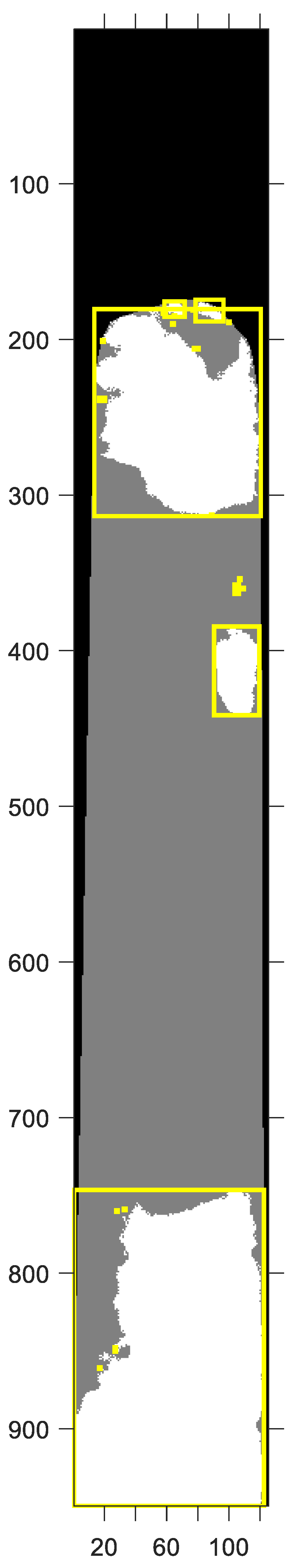
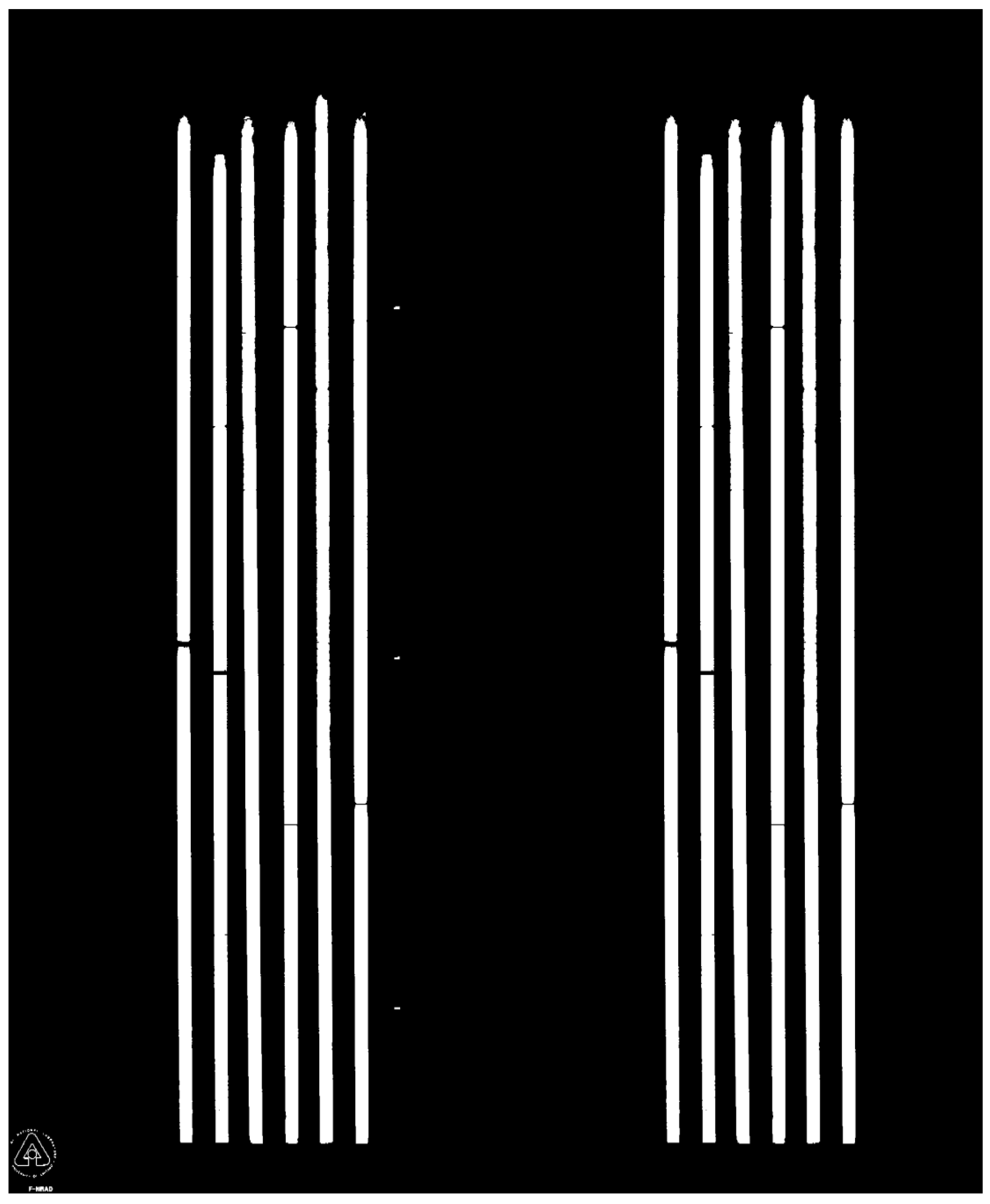
The output of the pins’ identification step is an image with bounding boxes for all pins and their parts. A bounding box is a rectangle that completely encompasses an image region and is used to describe a region’s location on the image. It is based on the extreme coordinates of an image region, and those coordinates are byproducts of the region labeling algorithm. Having identified bounding boxes for the fuel pins, we can also identify bounding boxes for the porosity region on top of the pins, as shown in Figure 7. The porosity regions’ bounding boxes are simply extensions of fuel pins bounding boxes to the top edge of the image. Figure 7 also has numeric labels for different identified pin regions. Due to pins cracking, some pins consist of disjoined regions; for example, pin T492, fourth from the right, has three different regions, while pin T408 consists of a single region. Figure 6 shows a zoomed-in part of the top of Figure 7 for a more thorough inspection of the bounding boxes. As can be seen in Figure 8, the porosity’s bounding boxes start at the top edge of fuel pins boxes and protract vertically until the very end of the original image. Some original images have a white border around the image. If that border is part of the porosity’s bounding box, it is removed prior to further analysis. As can be seen, the original image in Figure 8 has a border on top of the image. Horizontally, the widths of the porosity’s bounding boxes are the same as the widths of the pins’ bounding boxes. Some of the pins in Figure 8 have their bounding boxes in the upper part wider than the pins themselves. This is because pins are not always placed perfectly vertically when radiographed and also due to pins’ irradiation deformations. In Figure 8, the third and fifth pins from the right are distorted and have wider bounding boxes. Since the porosity’s bounding boxes are just extensions of pins bounding boxes, further image processing is required to extract pixels corresponding to the porous matter from the porosity bounding boxes.

3.3. Porosity Localization

The same algorithm of intensity adjustment and binarization is applied to the porosity’s bounding boxes to identify pixels corresponding to the porous matter. Based on histogram analysis of porosity’s bounding boxes, the low-intensity adjustment threshold is set to 102 while the top-intensity adjustment threshold is the same as before and equals 204. Notice that the low threshold is smaller than the one used for pins identification. This is because a larger portion of gray-value pixels constituting the porous matter needs to be preserved. The binarization threshold is set to 51 to make sure that low-intensity porosity pixels are preserved in the binarized image. Selecting the binarization threshold is based on the analysis of the intensity-adjusted images of porosity bounding boxes. After binarization, the connectivity algorithm, as well as area-based thresholding, were applied to the porosity bounding boxes. Area-based filtering is necessary because the porous matter may have very small, isolated specks due to imaging noise, and those specks need to be ignored prior to calculating any parameters of the porosity. The area threshold was set to a very low value of just 10 pixels based on area histogram analysis. In contrast to area thresholding of the pins, though, small regions were not removed from the image but simply ignored during parameter calculations.

The binarized and area-based thresholded image of the porous matter corresponding to green bounding boxes in Figure 8 is shown in Figure 9. For comparison, the original image of the porosity bounding boxes is shown in Figure 8. Analysis of Figure 9 and Figure 10 reveals that the operations of intensity adjustment, binarization, and area thresholding retained major and minor regions containing porous matter. While some very low-intensity pixels were removed by these operations, the residual information is comprehensive enough to calculate different statistical characteristics of the porosity.

3.4. Porosity Parameters

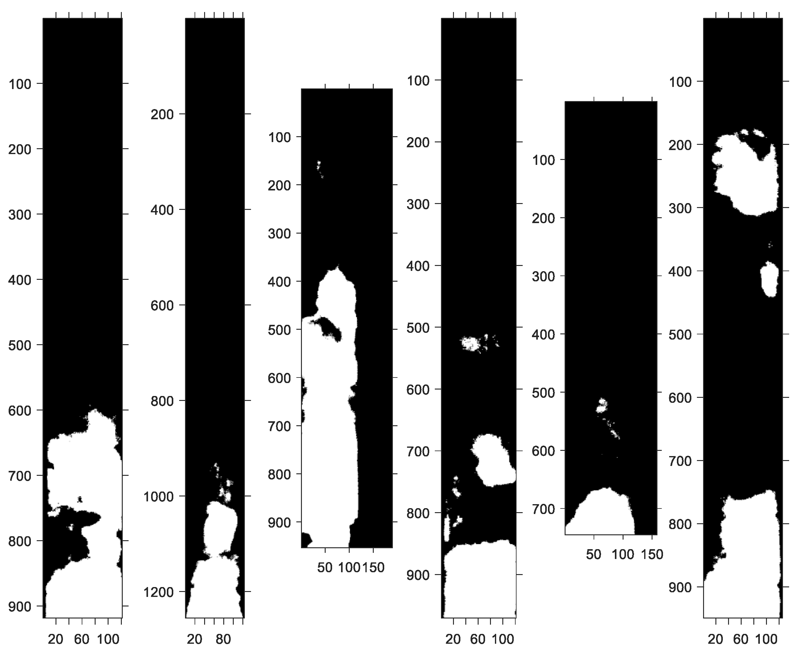
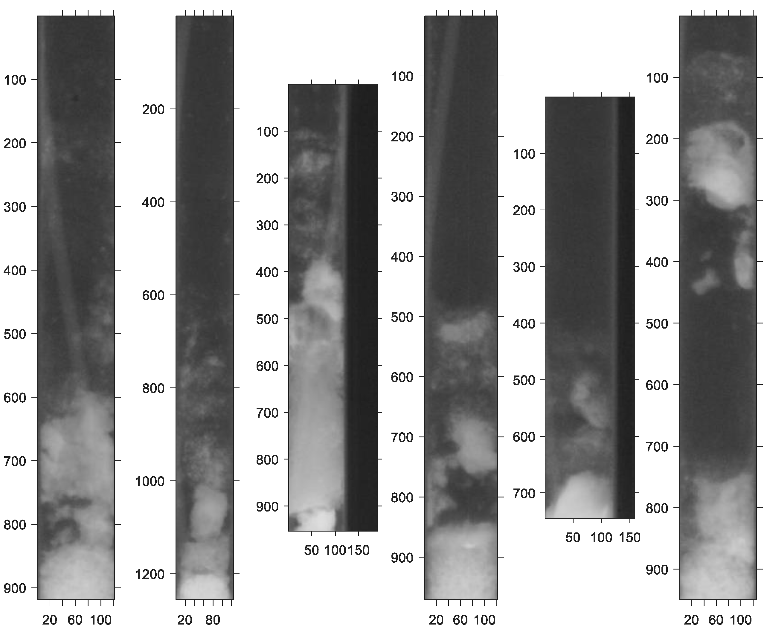
Arguably, the most important characteristic of the emerged porous matter is its span or length. Analysis of Figure 9 and Figure 10 reveals that the porosity consists of regions of different sizes and shapes represented as white pixels in Figure 9. The leftmost pin T446 in Figure 9 and Figure 10 has a single porosity region occupying about one-third of the bounding box. On the other hand, the rightmost pin T447 has two large distant disjoint regions with a smaller porous blob between those regions. Other pins have porous regions of various sizes and spans. In view of these different appearances, two different measures of the length can be used. Both measures first find the porous region, which is the furthest from the bottom of the bounding box. Only regions passing the area threshold test are eligible for consideration.

After such a region is identified for each bounding box, the center of the mass of this region is determined using a centroid-finding algorithm. If each pixel is assigned a mass of unity, then the standard formula for a center of mass of a two-dimensional shape can be written as:

$$X_c=\frac{1}{N}\sum _{i=1}^N{x}_i,\hspace{1em}{Y}_c=\frac{1}{N}\sum _{i=1}^N{y}_i$$

(2)

where $X_c$ and $Y_c$ are coordinates of the center of mass, $N$ is the total number of pixels in the region, and $x_i$ and $y_i$ are coordinates of $i^{th}$ pixel. These coordinates are used to determine the length of the span of the porous matter within the bounding box for each pin. 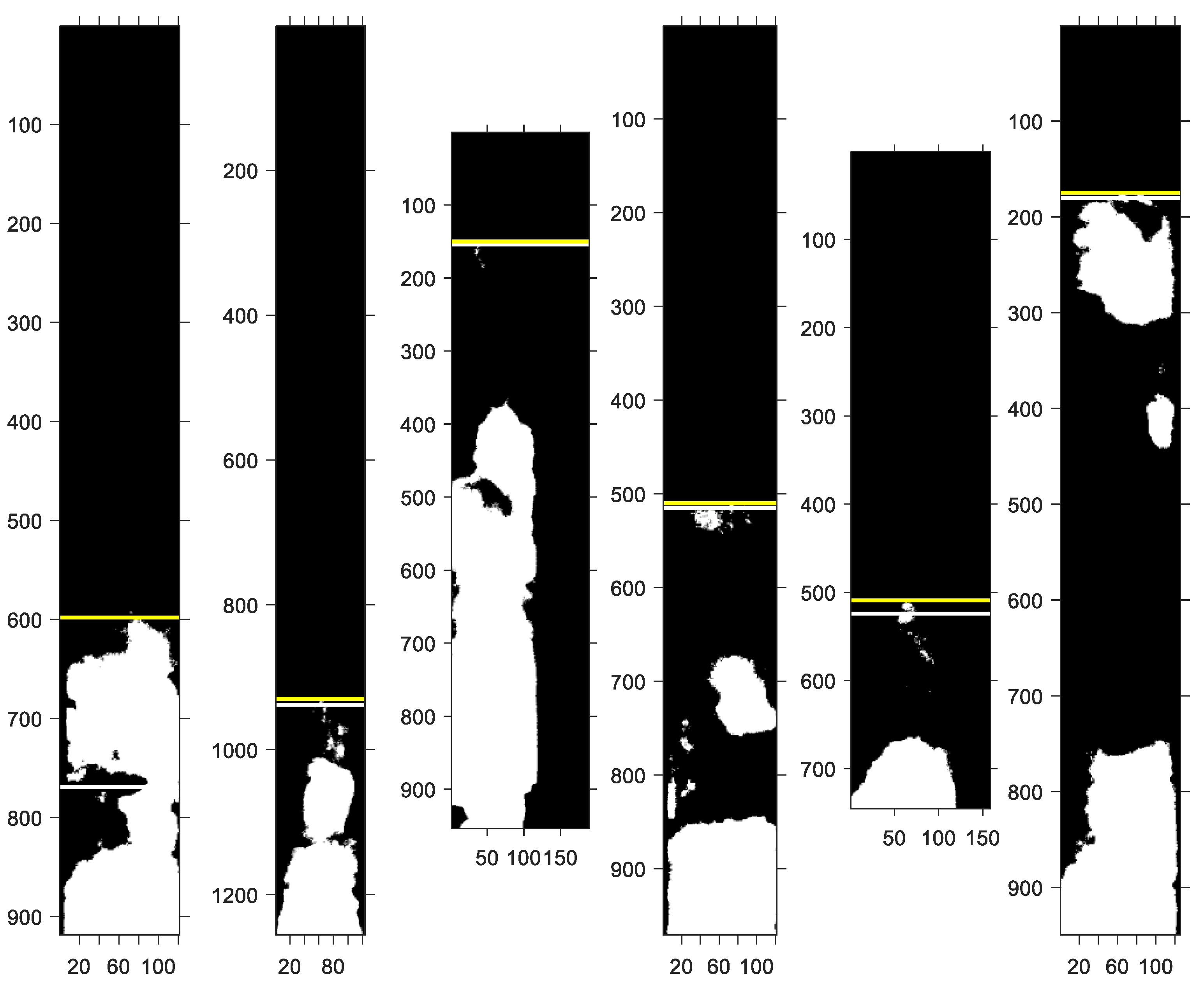The length is measured as the pixel distance between the bottom border of the bounding box and the centroid’s $Y_c$ coordinate. The distance measured in pixels is converted to centimeters using the ruler present in each original image. This length can be called centroid length. On the other hand, the length of the porosity span can be measured as the distance between the bottom of the bounding box and the furthest pixel of the most distant porosity region. This distance is called extrema distance. The two distances can be different, as evident from Figure 11.

The yellow lines in Figure 11 are drawn through the extrema coordinates of the furthest porosity region, while white lines are drawn through the centroid coordinates. Notice that the centroid coordinates are always lower than the extrema coordinate, as expected. The largest difference between the two measurements is for the leftmost pin, T446. This pin has a single porous region extending from the bottom of the bounding box to the y-pixel coordinate of about 600. In this situation, the coordinates are far apart and produce significantly different results. On the other hand, all other pins have two different measures close to each other. The advantage of using the extrema coordinates is that they always measure the longest span of the porosity. However, it can also slightly overestimate the span when the furthest region is small, as in pins T486 and T408 (second and third from the left). Another reason for using two measurements for the length of the porosity is to provide a “sanity” check for calculations. While the two measures can be different, they must be highly correlated, and one of them must be consistently lower than the other. Such verification is very useful, as the sheer volume of processed images and pins does not allow for a detailed visual inspection of calculated results.

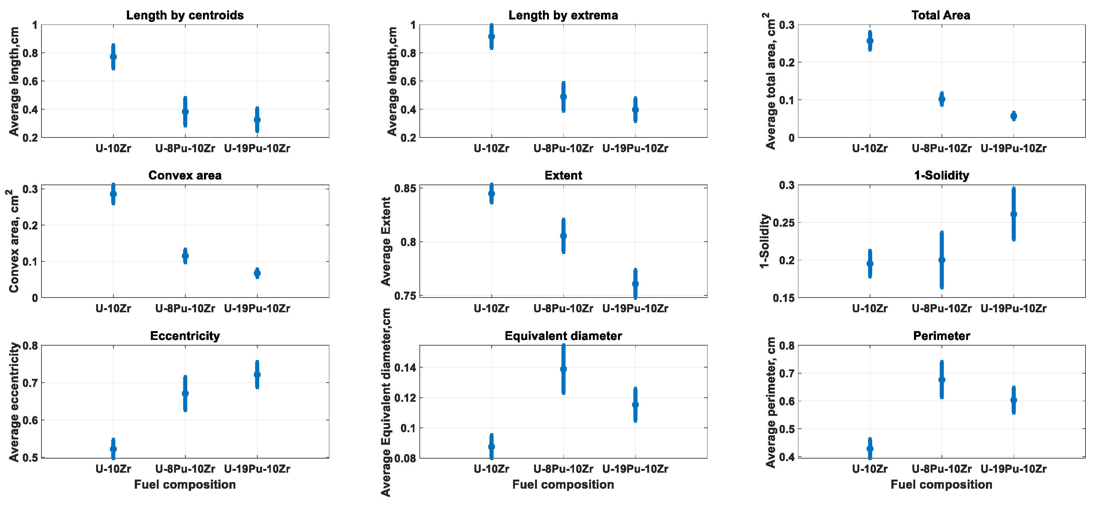
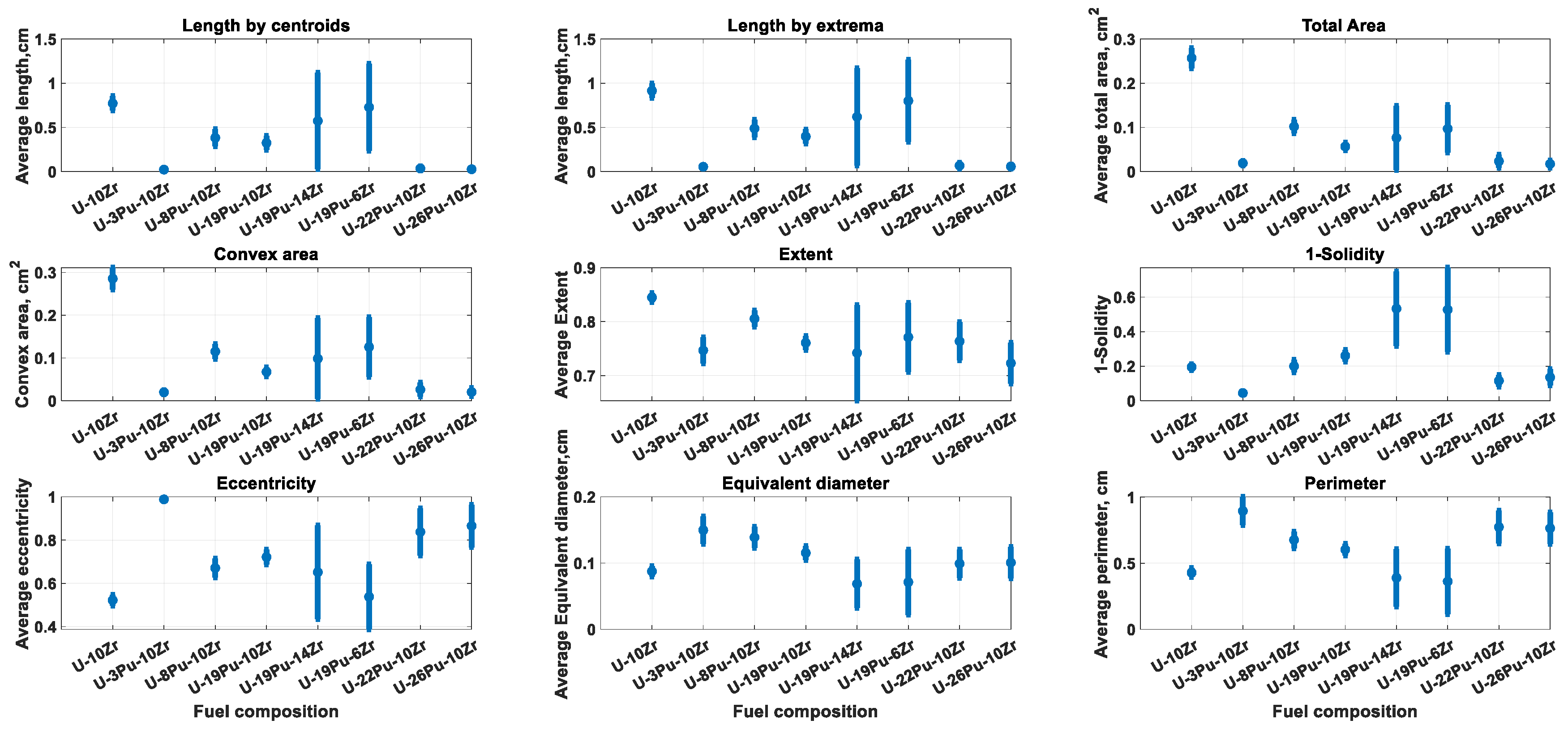
While being the most important characteristic of porosity, its span does not fully quantify such properties as volume, solidity, and shape. To account for these properties, the following parameters presented in

Table 2. Parameters of the porosity calculated in this study.

Property	Description
Total area of the porous matter, cm2	Calculates the total number of pixels in all porosity regions and converts the number to cm2. Measures the total amount of porous matter present for each pin.
Total convex area of the porous matter, cm2	Calculates the area of the smallest convex polygon containing all porosity regions, called convex hull. Measures the dispersion of the porosity for each pin.
Solidity, unitless	Total area/total convex area; calculates the ratio of the porous matter area within the convex hull to the area of convex hull. Solidity is bounded from above by one.
Average extent, unitless	Total area/region’s bounding box area; extent is bounded from above by one. Measures the density of the porous matter region within its bounding box.
Average eccentricity, unitless	Eccentricity measures the average roundedness of the porosity regions. For a single region, the eccentricity is equal to 0 if the region is a perfect circle, and it is 1 if the region is a line segment. The eccentricity and average eccentricity are between 0 and 1.
Average equivalent diameter, cm	Diameter of a circle with the same area as a porosity region averaged over all regions within bounding box. Measures granularity of the porous matter.
Average perimeter, cm	Measures perimeter of each porosity region for a pin and takes the average.

were calculated for each pin separately.

While many parameters in Table 2 are self-explanatory, the calculations involving the convex hull and extent may benefit from further clarification. Figure 12 shows pin T447 with porosity regions, their corresponding bounding boxes, and a convex hull.

The total area of the porous matter is the area occupied by white pixels in Figure 12. The convex hull is the gray area, which includes all the porosity regions. The bounding boxes for each porosity region are shown in yellow. For small regions, the bounding boxes look like yellow dots in Figure 10. The area of the black rectangle is the area of the bounding box for all porosity regions. This is the box shown in green in Figure 5 and Figure 6. The second parameter in Table 2 is the area covered by gray pixels, which also includes all white pixels. Solidity is the ratio of the white area to the gray area. Extent is the ratio of the porosity region’s area to the area of its bounding box, as shown in yellow. 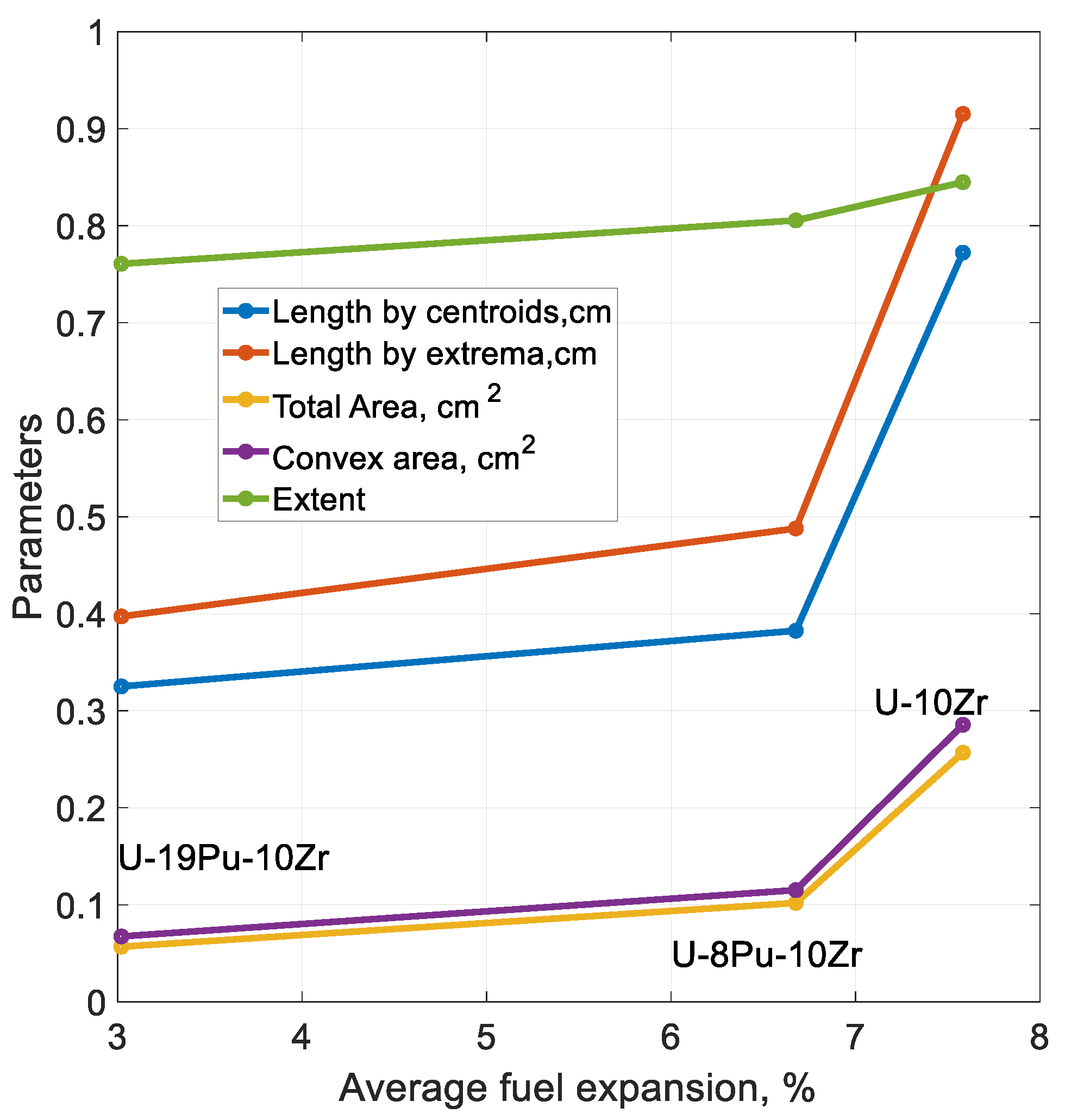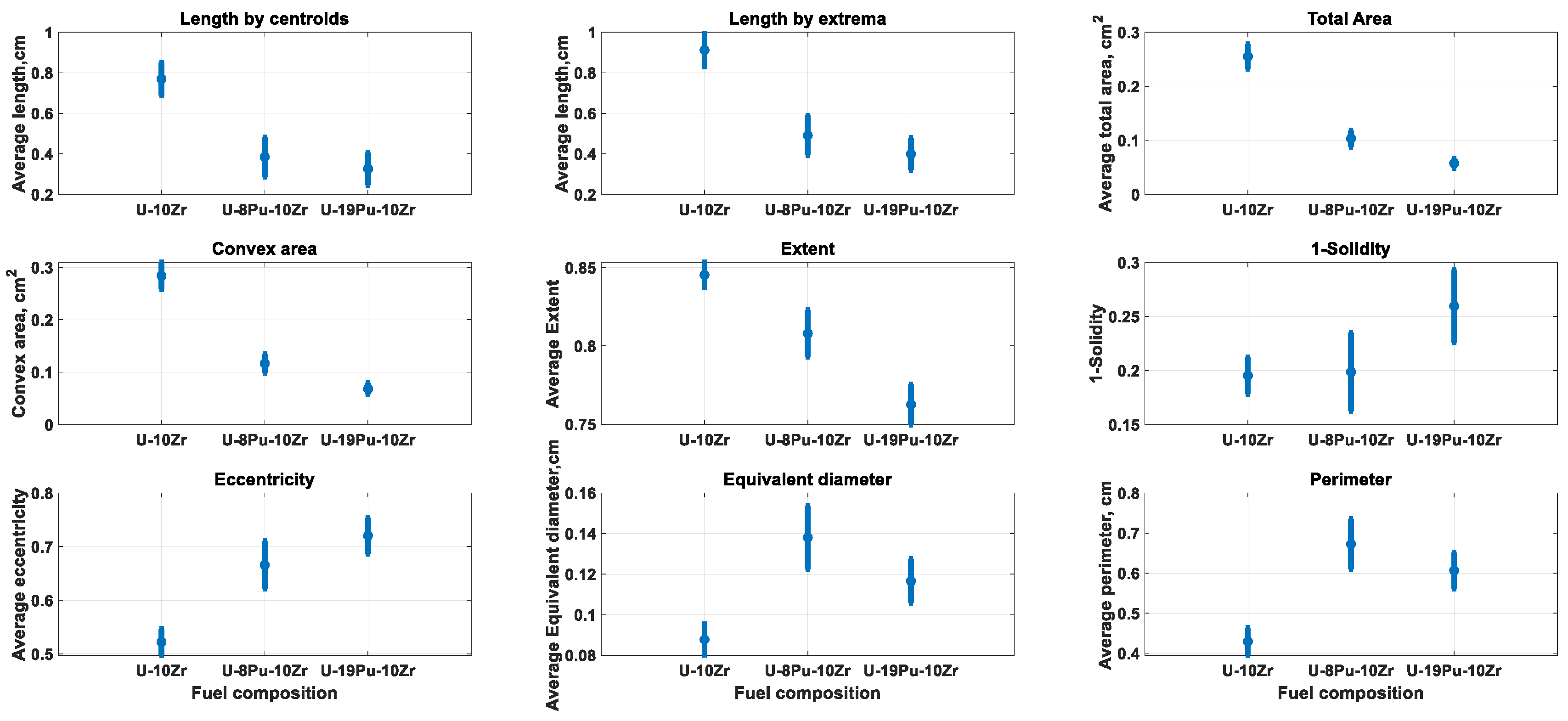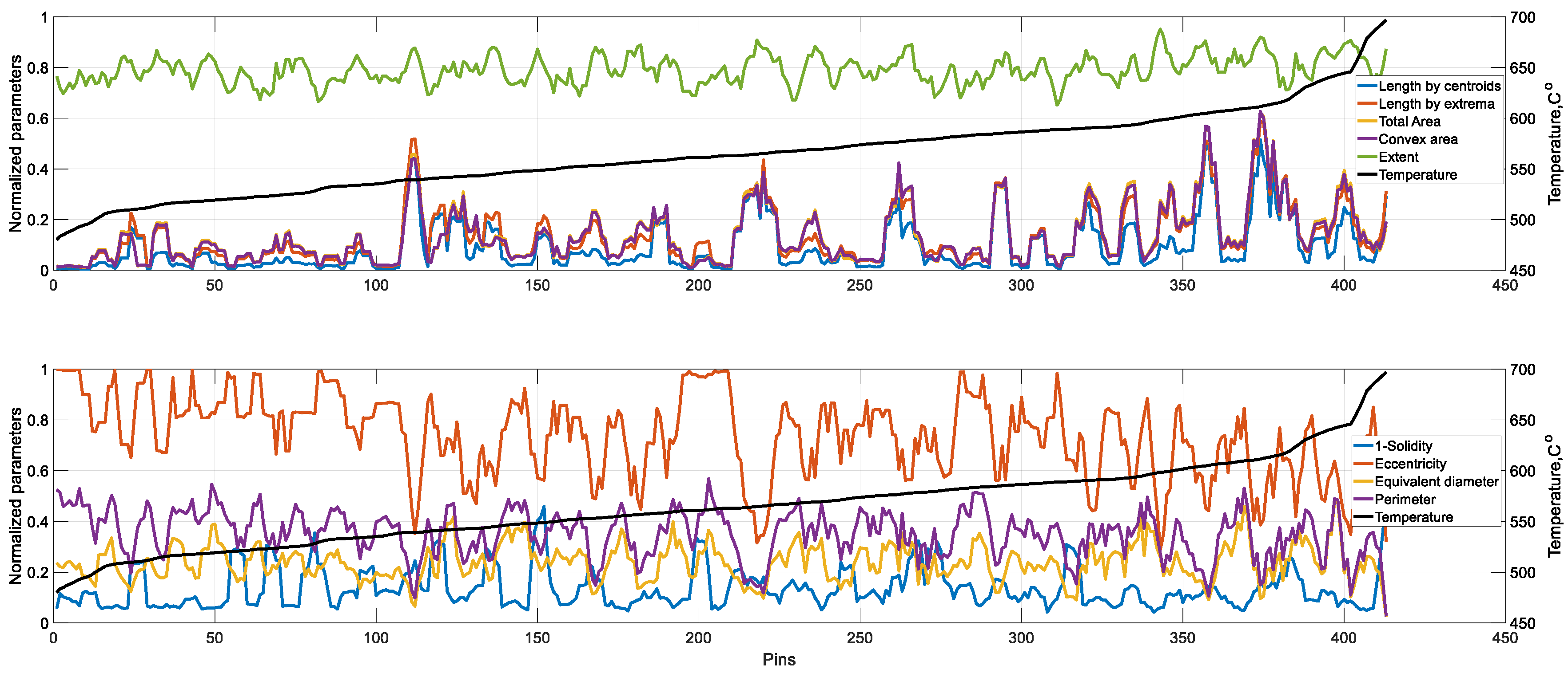For example, for the porosity region in Figure 10 with a y-coordinate around 400, the extent parameter is calculated as the ratio of the white area inside the yellow rectangle to the total area of the yellow rectangle. The extent is calculated for each porosity region separately, and the average value is taken to report as the extent parameter for a pin. The calculated porosity parameters were studied as functions of fuel composition, cladding temperatures, fuel expansion, and fuel burnup.

4. Results

4.1. Porosity and Fuel Composition

First, we analyze the dependence of porosity parameters on fuel composition. While eight different fuel compositions were analyzed in this study, three major compositions constitute over 90% of all pins. Figure 13 shows the dependence of nine porosity parameters discussed in Table 2 on three major fuel compositions. Notice that the solidity is plotted for complementary value as “1-Solidity” since this value better describes porosity. Figure 14 shows the same dependencies for all eight types of fuel considered in this study. The three parameters in the top row of Figure 13 and Figure 14, as well as two leftmost parameters in the second row of the same figures, in general, reflect the volume of the porous matter and hence can be labeled as volume parameters. In contrast, the remaining four parameters, in general, describe the granularity or graininess of the porous matter and can be called granularity parameters. This dichotomy is important as parameters demonstrate similar behavior within groups, which is analyzed in the Discussion section.

4.2. Porosity and Fuel Expansion

It is known that adding Pu stunts the axial fuel expansion [20], and the percent of Pu content correlates negatively with axial fuel expansion. Figure 15 shows the correlation between the percent of fuel expansion and five volume parameters for three major types of fuel. The algorithm used to determine axial fuel expansion is described in [20].

The x-axis in Figure 15 represents an average percent of fuel expansion for fuels U-19Pu-10Zr, U-8Pu-10Zr, and U-10Zr plotted from left to right. Notice that in this plot, the axial swelling is plotted in decreasing order of the Pu content. The lowest swelling, around 3%, is for Pu-rich U-19Pu-10Zr, while the highest one is for U-10Zr, at around 7.6%. The lines between the dots in Figure 13 are linear interpolations that were added for improved visibility. Each dot corresponds to the average axial fuel expansion for the corresponding fuel composition. Figure 16 shows the dependence of the granularity parameters for three major types of fuel.

4.3. Porosity and Cladding Temperature

The results presented so far did not consider dependencies on cladding temperatures or fuel burnup. Unfortunately, the number of pins with available cladding temperatures is much smaller, with only 413 for all eight fuel compositions. This shortage limits analyzing temperature dependencies and does not allow a meaningful analysis of the data for three major fuel compositions. The dependency of fuel axial expansion on cladding temperature was analyzed and is presented in Figure 17. The dependency is shown for three main fuel types, and it can be argued that the percent of fuel expansion undergoes an increase in temperature range between 500 and 550 °C and then saturates for higher temperatures. Otherwise, the dependency is weak and does not show any substantial correlations for either fuel type. Since the peak cladding temperature does not show any substantial correlation with fuel composition, which was shown to be correlated with porosity parameters, no further investigation of these temperature dependencies for different fuel types was undertaken.

The next step is to analyze the dependency of porosity parameters on cladding temperatures for all fuel types and all pins with available temperature values regardless of fuel type. To perform this analysis, the pins with available temperature values were sorted by their peak cladding temperatures in ascending order, and their porosity parameters were plotted along with the temperature values, as shown in Figure 18. The peak cladding temperature of pins increases from left to right in Figure 18. All parameter values were divided by their corresponding maximum to bring them to the same scale for plotting. The peak cladding temperature is plotted with a separate y-axis on the right.

4.4. Porosity and Burnup

The final dependency examined in this paper is the dependency between pins’ burnup values and porosity parameters. Out of 1097 pins, the burnup values were available for 1044. Pins had two burnup values: average and peak. The peak value was used in this paper to study the dependencies and generate results. The real physical values of peak burnups for reported pins ranged from 0.35 at% to 15 at%. A similar approach to studying temperature dependencies was used for burnup results. The pins’ burnup values were sorted in ascending order, and porosity parameters were plotted as functions of the pins’ burnup values, as shown in Figure 19. All plotted variables were normalized by their maxima. The burnup values are plotted with a separate ordinate axis on the right.

4.5. Sensitivity Analysis

The image processing algorithm used in this paper has a number of tunable parameters that may critically affect its performance. The most important parameter is the binarization threshold, which was selected to be 218 and used for all images in this paper. The selection was based on an analysis of the images’ histograms. However, to demonstrate the robustness of the algorithm and the reproducibility of the results, the sensitivity analysis was performed by randomly changing the binarization threshold using a threshold value selected from a truncated normal distribution. The truncated normal distribution had a mean value of 218 and a standard deviation of 5. The histogram of the thresholds generated for all images is shown in Figure 20. The threshold values for 185 images span the range between 205 and 234. Each image was binarized with its own threshold, and the rest of the image processing algorithms remained the same. If the algorithm is insensitive to minor variations in the binarization threshold value, it demonstrates its robustness and repeatability of the results if one opts for a different threshold selection algorithm. Figure 21 shows the dependency of the porosity parameters on three fuel types when a randomly selected binarization threshold was applied to each image. Figure 21 should be compared with Figure 13, where the same dependencies are plotted for the fixed threshold. The comparison of the two figures demonstrates that changing the binarization threshold did not change the mean value of the nine porosity parameters for three major types of fuel. It shows the relative robustness of the algorithm to the variations in binarization threshold values and the repeatability of the results if a different threshold selection method is preferred.

5. Discussion

We start the discussion of our results with the dependency of the porosity on fuel types, as shown in Figure 13 and Figure 14. Notice that the three parameters plotted in the top row of Figure 13, as well as the first two parameters from the second row, exhibit a similar pattern as a function of Pu content. Specifically, the higher Pu content corresponds to the lower value of the parameter. These five parameters reflect the total amount of porous matter formed on top of the fuel pins and, in general, are in agreement with results reported in [12] obtained with a smaller number of pins and without automatic processing. As mentioned above, these five parameters are called volume parameters. It seems that adding Pu suppresses the production of porous matter regardless of fuel burnup, fuel axial expansion, or cladding temperature. The remaining four parameters describe the granularity of the porous matter and, in general, show either an upward (“1-Solidity” and “Eccentricity”) or a downward parabola behavior (“Equivalent diameter” and “Perimeter”).

As for the eight types of fuel presented in Figure 14, the U-19Pu-14Zr and U-19Pu-6Zr have very few pins, and as a result, the confidence intervals are wide, and it is statistically unreliable to make any conclusions about the behavior of porous matter for these types of fuel. However, for U-22Pu-10Zr and U-26Pu-10Zr fuels, the number of pins is sufficient to produce tight confidence intervals for many porosity parameters. It can be seen that the last two fuel types with the largest Pu content continue the trend set by the three major fuels’ compositions for volume parameters. As far as the granularity parameters are concerned, they all show a similar pattern when plotted for all eight fuels. While the parameter values for U-3Pu-10Zr do not follow the pattern as a function of fuel type, for example, the length parameters for U-3Pu-10Zr show lower values than length parameters for fuels with larger Pu content, they nevertheless show a consistent pattern for both volume and granularity parameters.

Figure 15 and Figure 16 show dependencies for two groups of parameters on fuel expansion. It can be seen that the parameter values have a high positive correlation with the percent of fuel axial expansion, with correlation values between 0.74 and 0.96 for different parameters. The highest value of 0.96 is for the “Extent” parameter. The granularity parameters all demonstrated consistent negative correlations with the percent of axial fuel expansion ranging from −0.24 for “Perimeter” to −0.99 for “1-Solidity”. The latter result indicates an almost linear dependency between the degree of porosity and axial fuel expansion, with U-19Pu-10Zr having the highest degree of porosity and U-10Zr having the lowest.

Analyzing correlations between porosity parameters and axial fuel swelling for all eight types of fuel compositions is complicated by the insufficient statistical samples for some more rare fuel types. However, even in this case, there are significant positive correlations between axial swelling and extent, with a correlation coefficient equal to 0.82 and a convex area with a correlation coefficient equal to 0.63 (plots not shown).

The dependency of porosity parameters on peak cladding temperatures regardless of fuel type and burnup is shown in Figure 18. Since pins’ parameters are plotted in the order of increasing temperature values, we expect to see either positive or negative parameter trends with respect to temperature if any dependency exists. However, as can be seen in Figure 18, no such trends are visible, indicating the lack of linear or any other dependency between cladding temperature and porosity parameters. The only parameter that arguably shows a downward trend as temperature increases is the eccentricity parameter. It also shows that the cladding temperature has a very low degree of variability in comparison to porosity parameters, and this may explain the lack of clear dependency between the two. On the other hand, Figure 18 shows a very high degree of correlation among volume parameters (except extent) and granularity parameters. This gives an indirect assurance to the quality of parameter calculations as it is expected that volume and granularity parameters must have a high correlation within those two groups.

The top panel of Figure 19 shows that there is a positive correlation between four volume parameters and burnup, with an average correlation coefficient of 0.55. The extent parameter does not show any correlation with burnup, with the correlation coefficient being 0.37. On the other hand, none of the granularity parameters show any significant correlation with burnup values, as is evident from the bottom panel in Figure 19.

Finally, Figure 20 and Figure 21 demonstrate the sensitivity of the algorithm to the binarization threshold. Figure 21, when compared with Figure 13, shows that the results are practically identical, which demonstrates that the algorithm is robust to minor variations in its critical parameter and can be used if a different threshold selection method is applied to process the images.

6. Conclusions

Understanding the properties and formation mechanisms of porous matter formed at the top of the metallic fuel pins may have a significant impact on future reactor design and fuel modeling. This paper presents the most comprehensive statistical analysis of the properties of the porosity to date and validates the results reported previously on smaller samples. Eight different fuel compositions and nine porosity parameters were studied. It is shown that the formation of the porous matter depends on the number of parameters, such as fuel composition, fuel axial expansion, cladding temperature, and burnup. In contrast to previously published results, which considered a single porosity parameter (length), nine different porosity parameters were analyzed and studied. The nine parameters can be dichotomized as volume and granularity groups, with five parameters characterizing the overall amount of porous matter called volume parameters and four parameters describing the “sponginess/fluffiness” of the porous matter called granularity parameters. The volume parameters demonstrated similar correlations as functions of fuel composition and axial expansion. As a function of fuel composition for three main fuel types, the overall volume of produced porous matter showed a negative correlation with Pu content, which confirmed the results reported in the previous study. On the contrary, the granularity parameters demonstrated either a negative correlation or nonlinear dependency on the Pu content. These results are new and have not been previously reported. In general, these conclusions are valid for dependencies found for all eight types of fuel compositions.

It was also shown that the volume parameters are positively correlated with fuel axial expansion when parsed by fuel type. This result is expected as it is known that the axial fuel expansion is stunted by adding Pu. The granularity parameters are found to be mostly negatively correlated with axial fuel expansion. The cladding temperature was found to be a weak predictor for the formation of porous matter in previous publications, and this conclusion is confirmed in this study. Finally, it was found that four out of five volume parameters show a positive correlation with fuel burnup percent, while the granularity parameters show no significant correlation. The sensitivity analysis of the binarization threshold demonstrated that the algorithm performance is robust to minor variations in the selection of the binarization threshold. Also, the algorithm is robust in selecting the threshold for the morphological opening of the image.

The proposed approach to the analysis of fluff formation in metallic fuels has some limitations imposed by the quality of raw images. For example, if raw images are too dark or too bright, the proposed technique may have difficulties selecting appropriate thresholds. While we demonstrated that the threshold selection does not affect the final results dramatically, the very existence of the binarization threshold, in this case, can be called into question as, ultimately, the image does not have a “true” threshold separating fluff from pins, and it is always a judgment call. However, as was pointed out in the introduction, the ultimate goal of this approach is to provide objective and repeatable results for the analysis of irradiated fuel pins. All works performed so far were based on empirical visual analysis of the images, and hence, their results are dependent on the analyst, their experience, and knowledge. This work removes such subjectivity from the reported results. If the existence of a “true” threshold separating fluff from fuel is postulated, then the natural future extension of this work would be selecting the threshold based on the minimization of statistical risk between “true” and the estimated threshold, which can be accomplished using existing statistical techniques.

References

1. Crawford, D.C.; Porter, D.L.; Hayes, S.L. Fuels for sodium-cooled fast reactors: U.S. perspective. J. Nucl. Mater. 2007, 371, 202–231. [Google Scholar] [CrossRef]
2. Crawford, D.C.; Porter, D.L.; Hayes, S.L.; Meyer, M.K.; Petti, D.A.; Pasamehmetoglu, K. An approach to fuel development and qualification. J. Nucl. Mater. 2007, 371, 232–242. [Google Scholar] [CrossRef]
3. Idaho National Laboratory. Work Planning and Control Assessment at the Idaho National Laboratory. Nuclear Materials Experiments Execution Process. LWP-20700, Rev. 1, Lab-Wide Procedure, Manual: 20—Research Management System; Office of Enterprise Assessments U.S. Department of Energy: Washington, DC, USA, October 2019; p. 3. [Google Scholar]
4. Porter, D.L.; Tsai, H. Full-length U-xPu-10Zr (x = 0, 8, 19) fast reactor fuel pin test in FFTF. J. Nucl. Mater. 2012, 427, 46–57. [Google Scholar] [CrossRef]
5. Porter, D.L.; Chichester, H.J.M.; Medvedev, P.G.; Hayes, S.L.; Teague, M.C. Performance of low smeared density sodium-cooled fast reactor metal fuel. J. Nucl. Mater. 2015, 465, 464–470. [Google Scholar] [CrossRef]
6. Tsai, H.; Cohen, A.B.; Billone, M.C.; Neimark, L.A. Irradiation performance of U-Pu-Zr metal fuels for liquid-metal-cooled reactors. In Proceedings of the 3rd International Conference on Nuclear Engineering (ICONE-3), Kyoto, Japan, 23–27 April 1995. [Google Scholar]
7. Pahl, R.G.; Lahm, C.E.; Hayes, S.L. Performance of HT9 clad metallic fuel at high temperature. J. Nucl. Mater. 1993, 204, 141–147. [Google Scholar] [CrossRef]
8. Hofman, G.L.; Pahl, R.G.; Lahm, C.E.; Porter, D.L. Swelling behavior of U-Pu-Zr fuel. Metall. Trans. 1990, 21A, 517–520. [Google Scholar] [CrossRef]
9. Hofman, G.L.; Walters, L.C.; Bauer, T.H. Metallic fast reactor fuels. Prog. Nucl. Energy 1997, 31, 83–110. [Google Scholar] [CrossRef]
10. Galloway, J.; Unal, C.; Carlson, N.; Porter, D.; Hayes, S. Modeling constituent redistribution in U-Pu-Zr metallic fuel using the advanced fuel performance code BISON. Nucl. Eng. Des. 2015, 286, 1–17. [Google Scholar] [CrossRef]
11. Di Lemma, F.G.; Wright, K.E.; Capriotti, L.; Zabriskie, A.X.; Winston, A.J.; Jensen, C.B.; Wachs, D.M. Investigation of fuel microstructure at the top of a metallic fuel pin after a reactor overpower transient. J. Nucl. Mater. 2021, 544, 152711. [Google Scholar] [CrossRef]
12. Fay, J.; Di Lemma, F.; Gribok, A.; Paaren, K.; Medvedev, P.; Capriotti, L.; Porter, D.; Lian, J. An analysis of fluff formation in metallic fuel via data analyzes from EBR-II experiments and BISON fuel code modeling. J. Nucl. Mater. 2022, 567, 153813. [Google Scholar] [CrossRef]
13. Rahn, T.; Capriotti, L.; Di Lemma, F.; Trowbridge, T.L.; Harp, J.M.; Aitkaliyeva, A. Investigation of constituent redistribution in U-Pu-Zr fuels and its dependence on varying Zr content. J. Nucl. Mater. 2021, 557, 153301. [Google Scholar] [CrossRef]
14. Craft, A.E.; Hilton, B.A.; Papaioannou, G.C. Characterization of a neutron beam following reconfiguration of the neutron radiography reactor (NRAD) core and addition of new fuel elements. Nucl. Eng. Technol. 2016, 48, 200–210. [Google Scholar] [CrossRef]
15. Recommendation ITU-R BT.601-7 Studio Encoding Parameters of Digital Television for Standard 4:3 and Wide Screen 16:9 Aspect Ratios; International Telecommunication Union: Geneva, Switzerland, 2011.
16. Gonzalez, R.C.; Woods, R.E. Digital Image Processing; Addison-Wesley: Reading, MA, USA, 1993. [Google Scholar]
17. Otsu, N. A Threshold Selection Method from Gray-Level Histograms. IEEE Trans. Syst. Man Cybern. 1979, 9, 62–66. [Google Scholar] [CrossRef]
18. He, L.; Ren, X.; Gao, Q.; Zhao, X.; Yao, B.; Chao, Y. The connected-component labeling problem: A review of state-of-the-art algorithms. Pattern Recognit. 2017, 70, 25–43. [Google Scholar] [CrossRef]
19. He, L.; Chao, Y.; Suzuki, K. Two efficient label-equivalence-based connected–component labeling algorithms for three-dimensional binary images. IEEE Trans. Image Process 2008, 20, 2122–2134. [Google Scholar]
20. Gribok, A.V.; Porter, D.L.; Paaren, K.M.; Gale, M.D.; Middlemas, S.C.; Lybeck, N.J. Automatic information extraction from neutron radiography imaging to estimate axial fuel expansion in EBR-II. J. Nucl. Mater. 2021, 557, 153250. [Google Scholar] [CrossRef]
Figure 1. Flow chart of image processing steps.
Energies 17 01990 g001
Figure 2. Original grayscale radiography image of X425B, pins T446, T486, T408, T492, T478, and T447 (left to right). The six pins (left to right) have the following fuel compositions: U-8Pu-10Zr, U-19Pu-10Zr, U-10Zr, U-8Pu-10Zr, U-10Zr, and U-8Pu-10Zr.
Energies 17 01990 g002
Figure 3. Longitudinal cross-cuts for raw and intensity-adjusted images along with respective histograms and intensity-mapping function. (A) is image cross cut along the magenta line shown in the previous figure. (B) is histograms of the original and intensity-adjusted images. (C) is intensity mapping function.
Energies 17 01990 g003
Figure 4. From left to right: contrast-adjusted, binarized, and quantized radiography images of X425B pins T446, T486, T408, T492, T478, and T447. Small bright areas of high intensity pixels are circled in yellow.
Energies 17 01990 g004
Figure 5. The 4-connectivity (left) and 8-connectivity (right) diagrams for neighboring pixels. The pixels marked black are considered connected to the pixel of interest marked gray.
Energies 17 01990 g005
Figure 6. Side-by-side comparison of binarized image and the area-thresholded binarized image of X425B pins T446, T486, T408, T492, T478, and T447.
Energies 17 01990 g006
Figure 7. Original image of X425B pins T446, T486, T408, T492, T478, and T447, with superimposed fuel pin bounding boxes and pin region numbers. The green bounding boxes are porosity region bounding boxes.
Energies 17 01990 g007
Figure 8. Top part of original image of X425B with superimposed pins and porosity regions’ bounding boxes.
Energies 17 01990 g008
Figure 9. Binarized and area-thresholded images of porous matter formed on top of the fuel pins T446, T486, T408, T492, T478, and T447 of experiment X425B.
Energies 17 01990 g009
Figure 10. Original images of porous matter formed on top of the fuel pins T446, T486, T408, T492, T478, and T447 of experiment X425B.
Energies 17 01990 g010
Figure 11. Two distance measures to determine the prolongation of the porous matter on top of the fuel pin. The yellow line is the extrema, and the white line is the centroid measures.
Energies 17 01990 g011
Figure 12. Convex hull of pin T447 porosity regions along with bounding boxes for each porosity region.
Energies 17 01990 g012
Figure 13. Dependence of nine porosity parameters on three major types of fuels. The vertical bars are 95% confidence intervals.
Energies 17 01990 g013
Figure 14. Dependence of nine porosity parameters on eight types of fuel. The vertical bars are 95% confidence intervals.
Energies 17 01990 g014
Figure 15. Five volume parameters as functions of average axial fuel expansion for three major types of fuel. The three fuel compositions are shown on the graph next to their corresponding expansion values.
Energies 17 01990 g015
Figure 16. Five granularity parameters as functions of average axial fuel expansion for three major types of fuel. The three fuel compositions are shown on the graph next to their corresponding expansion values.
Energies 17 01990 g016
Figure 17. Dependency of fuel expansion on peak cladding temperature for three major types of fuel.
Energies 17 01990 g017
Figure 18. Dependence of porosity parameters on cladding temperature values.
Energies 17 01990 g018
Figure 19. Dependence of porosity parameters on pins’ burnup values.
Energies 17 01990 g019
Figure 20. Histogram of the binarization thresholds selected from truncated normal distribution.
Energies 17 01990 g020
Figure 21. Dependence of nine porosity parameters on three major types of fuels using randomly selected binarization thresholds. The vertical bars are 95% confidence intervals.
Energies 17 01990 g021