Article

Toward Prediction of Energy Consumption Peaks and Timestamping in Commercial Supermarkets Using Deep Learning

1
Department of Electrical and Computer Engineering, Western University, London, ON N6A 3K7, Canada
2
Neelands Group Ltd., Burlington, ON L7M 0V9, Canada
3
Department of Civil and Environmental Engineering, Western University, London, ON N6A 3K7, Canada
*
Author to whom correspondence should be addressed.
Energies 2024, 17(7), 1672; https://doi.org/10.3390/en17071672
Submission received: 13 March 2024 / Revised: 26 March 2024 / Accepted: 27 March 2024 / Published: 1 April 2024
(This article belongs to the Collection Feature Paper Collection: Energy and Buildings)

Abstract

:
Building energy consumption takes up over 30% of global final energy use and 26% of global energy-related emissions. In addition, building operations represent nearly 55% of global electricity consumption. The management of peak demand plays a crucial role in optimizing building electricity usage, consequently leading to a reduction in carbon footprint. Accurately forecasting peak demand in commercial buildings provides benefits to both the suppliers and consumers by enhancing efficiency in electricity production and minimizing energy waste. Precise predictions of energy peaks enable the implementation of proactive peak-shaving strategies, the effective scheduling of battery response, and an enhancement of smart grid management. The current research on peak demand for commercial buildings has shown a gap in addressing timestamps for peak consumption incidents. To bridge the gap, an Energy Peaks and Timestamping Prediction (EPTP) framework is proposed to not only identify the energy peaks, but to also accurately predict the timestamps associated with their occurrences. In this EPTP framework, energy consumption prediction is performed with a long short-term memory network followed by the timestamp prediction using a multilayer perceptron network. The proposed framework was validated through experiments utilizing real-world commercial supermarket data. This evaluation was performed in comparison to the commonly used block maxima approach for indexing. The 2-h hit rate saw an improvement from 21% when employing the block maxima approach to 52.6% with the proposed EPTP framework for the hourly resolution. Similarly, the hit rate increased from 65.3% to 86% for the 15-min resolution. In addition, the average minute deviation decreased from 120 min with the block maxima approach to 62 min with the proposed EPTP framework with high-resolution data. The framework demonstrates satisfactory results when applied to high-resolution data obtained from real-world commercial supermarket energy consumption.

1. Introduction

Trends and patterns of energy consumption have been widely studied by numerous researchers due to growing concerns about supply difficulties and global warming [1,2,3]. The International Energy Agency [4] has reported that the operations of buildings account for 30% of global final energy consumption and 26% of global energy-related emissions. In addition, the Global Alliance for Buildings and Construction [5] reported that the electricity consumption in building operations represents nearly 55% of global electricity consumption. Therefore, efficiency in building energy management has become a crucial strategy in the low-carbon economy [6,7,8], and being able to accurately predict power loads has emerged as a crucial part of preventing energy wastage and in developing effective power management blueprints [9]. Precise predictions benefit both the suppliers and consumers by enhancing power management, grid security, and load control [10]. Furthermore, the accurate forecasting of power loads serves not only the initial stage in addressing load management [11], but also establishes a baseline for predicting peak demand [12].
The electrical grid structure faces challenges in balancing the power flow between the production and consumption of energy. There is always a gap between the forecasted demand and the available capacity to avoid energy shortages. Peak demand prediction in energy smart grid management aims to improve such issues through power storage scheduling and demand flexibility. The ultimate objective of peak demand management is to achieve a balance between electricity supply and demand, thereby maximizing the overall benefits of the power system. In addition, accurate peak demand prediction helps with peak shaving and load smoothing. Enhanced efficiency in electricity production, stemming from decreased fluctuations in power demand, will also contribute to a reduction in the carbon footprint [13]. Overall, the precise forecasting of peak loads holds significant importance in various applications including network constraint management, peak shaving, and the scheduling of batteries and demand response. Considering that electricity consumption in commercial buildings has increased by 82% since 1979 [14], optimizing the load predictions is crucial in mitigating energy wastage in commercial building management.
The energy consumed by commercial buildings in the United States, encompassing office spaces, retail establishments, educational and healthcare facilities as well as lodging, primarily originated from electricity and natural gas, accounting for 60% and 34% of the total consumption, respectively [14]. Notably, electricity is the most commonly used energy source by commercial buildings in the United States, which is utilized in 95% of establishments, representing 98% of the total floorspace [15]. In commercial supermarkets, over 70% of the energy utilized is in the form of electricity, primarily dedicated to powering refrigeration equipment [16,17]. The remaining portion of the energy is allocated to tasks such as lighting, HVAC (heating, ventilation, and air conditioning), baking, and other supplementary services [18]. In such a scenario, refrigeration systems can be utilized as virtual batteries by increasing the energy consumption during low-demand hours and discharging during peak hours to smooth out the electricity consumption. Therefore, accurate predictions of the peak energy consumption as well as the time index are the key preconditions in promoting such load-shaving strategies. In this work, a novel approach is proposed that uses long short-term memory (LSTM) and multilayer perceptron (MLP) networks to predict both the peak energy demand as well as the time index based on the energy consumption data and weather information. The contributions of this work are summarized as follows:
  • An Energy Peaks and Timestamping Prediction (EPTP) framework is proposed as a novel approach for commercial building applications to predict not only the value of the peak energy consumption, but also the corresponding starting, peaking, and ending indices in various data resolutions.
  • The time indices are labeled with block maxima (BM) and base values to avoid long peak durations, especially in low-frequency data. The labeling of the time indices not only helps prevent prolonged durations, but also enables the second stage of training of the EPTP framework.
  • The proposed EPTP framework is also benchmarked using an existing open-source dataset and baselined with common indexing practices, where the performance of the EPTP framework is compared using hit rates and time deviations.
The rest of this work is organized as follows. Section 2 focuses on the existing methodologies for energy and peak demand predictions with potential gap areas. Section 3 introduces the overview of the MLP and LSTM structures and the corresponding hyperparameter tuning processes. Section 4 presents the proposed EPTP framework. Section 5 discusses the evaluation of the EPTP Framework with two databases. Finally, Section 6 concludes the research with key outcomes and future work.

2. Related Work

2.1. Energy Consumption Forecasting in Commercial Building

Demand forecasting can be classified into three categories: short-term, medium-term, and long-term [19]. By definition, short-term forecasts typically cover intervals from one hour to one week, medium-term forecasts span from one week to one year, and long-term forecasts extend beyond one year. The current research specifically focused on the short-term forecasting of energy consumption, hence, the literature review primarily concentrated on short-term forecasting within commercial building applications [20,21]. After reviewing the state-of-the-art models, it was observed that common methods for such tasks included variations or hybrid models of autoregression integrated moving average [22,23], support vector machine [24,25,26], and LSTM [27,28].
A hybrid model combining autoregression integrated moving average and support vector regression (SVR) was introduced to predict electricity consumption with various prediction horizons for an office building [23]. Their findings indicated that the performance of the proposed hybrid model excelled with a shorter prediction horizon, while the vanilla autoregression integrated moving average model exhibited better predictions for longer horizons. However, their proposed model was only tested on a small-scale dataset comprising 117 daily electricity consumption datapoints. The H-EMD-SVR-PSO hybrid model was proposed to improve the forecasting accuracy of a supermarket in Australia [24]. Their model employed empirical mode decomposition to decompose electric load data into nine intrinsic mode functions. The intrinsic mode functions were categorized into three groups and modeled separately using SVR with particle swarm optimization [25]. Their study concluded that the proposed H-EMD-SVR-PSO model achieved high accuracy and was easily interpretable. A comparison between LSTM and support vector machine models on a building with a significant commercial profile was conducted [28] with performance assessment using the mean absolute error (MAE), root mean squared error (RMSE), and mean absolute percentage error (MAPE). The study concluded that the LSTM model exhibited higher prediction accuracy when a sufficient amount of load data was available. However, in cases of limited training data and when prioritizing time cost, the overall performance favored the support vector machine model.
Based on the literature review on short-term forecasts in commercial buildings, the proposed framework incorporated LSTM as a baseline model for peak demand prediction. Aligning with the findings of [29], which identified three typical types of independent variables in commercial building energy models (i.e., weather, occupancy, and time), this work included weather information and time-related variables in the energy prediction modeling, considering data availability. To assess the performance of this work, common performance metrics such as MAE, RMSE, and MAPE, consistent with standard practices in energy prediction model evaluation, were employed.

2.2. Peak Demand Prediction

Peak demand prediction has gained increasing attention across various industries for load management and scheduling purposes. Studies in this domain, particularly focusing on residential houses and neighborhood energy management, have employed techniques such as the ensemble LSTM model [30], CNN sequence-to-sequence network [31], and cluster analysis [32]. In addition, the peak load demand in a distribution zone substation located in Australia was forecasted and concluded that the LSTM model could predict faster and more accurately compared with feed-forward neural networks and recurrent neural networks [33]. The hybrid complete ensemble empirical mode decomposition with adaptive noise for data decomposition and extreme gradient boosting for predicting energy consumption proposed by [34] were tested using the daily peak power consumption data from an intake tower. On a broader scale, research on peak demand forecasting has extended to include studies on power system networks [35], national grids [36], and daily electricity demand data [37,38].
Research on peak demand predictions has also directed its attention to commercial buildings. Ensemble models were proposed to predict next-day total energy consumption and peak power demand [39]. Their method employed a data mining-based approach, with variable selection for individual models based on recursive feature elimination, and optimization of ensemble models weighted using the genetic algorithm. Their study concluded that the accuracy of the ensemble model surpassed that of individual base models. However, it is worth noting that the prediction of the peak power demand was treated as a standalone task, with recursive feature elimination and genetic algorithm steps conducted independently of energy consumption prediction. Furthermore, the model did not incorporate the timing of peak demand, which is essential information for peak shaving strategies. A probabilistic regression model for the daily electrical peak demand was suggested in [40]. Their modeling approach involved using temperature and occupancy as predictors for electric demand. Their research concluded that the proposed method outperformed machine learning algorithms, specifically support vector machine, random forest, and MLP, when dealing with small datasets. However, the model was trained with only one datapoint for each feature per day, predicting only the maximum daily consumption and considering only the peak output value. An artificial neural network model with a Bayesian regularization algorithm was investigated for predicting day-ahead electricity usage in 15-min intervals [41]. Their results indicated that the proposed adaptive training methods could reasonably predict daily peak electricity usage. However, the peak hours were predefined by the suppliers and based solely on seasonal considerations.
The aforementioned methodologies employed various approaches to predict the magnitude of peak energy consumption, but the research did not focus on determining the specific index or timestamp corresponding to the peak occurrence. Conversely, daily electricity load peak demand was considered as the maximum value of the electricity power demand curve over one day [36]. They proposed a multi-resolution approach to forecasting both the magnitude and the timing of the peak demand occurrence. Their proposed algorithm was tested with a half-hourly demand resolution using the UK total national demand. The authors reported a mixed performance, particularly in peak timing forecasting, especially when employing a multi-resolution generalized additive model. Furthermore, another study proposed employing probabilistic forecasting with forecast fusion in the low-voltage network to predict peak density and timing [42]. Their proposed framework underwent testing using real smart meter data and a hypothetical low-voltage network hierarchy comprising feeders as well as secondary and primary substations. They concluded that the proposed framework based on generalized additive models for location, scale, and shape contrasts with non-parametric methods and yielded an average improvement of 5% compared to kernel density estimation.
From this literature review, it can be deduced that there is a notable gap in the exploration of the time index for peak demand within the domain of commercial building applications. Most studies primarily focused on predicting the magnitude of the peak value, neglecting the timestamp associated with the peak occurrence. This lack of emphasis on identifying timestamps is a common trend observed in commercial buildings and other applications such as residential houses. Additionally, the performance of the approaches in timestamp forecasting has shown mixed results, with some studies utilizing hypothetical networks rather than real-world applications. To address this gap, this paper acknowledges the significance of predicting both the magnitude and index of the peak, aiming to enhance smart grid management and operational planning [43]. The proposed framework goes beyond solely forecasting the peak demand value; it also focuses on predicting the timestamps for the starting, peaking, and ending indices specifically tailored for a commercial supermarket located in Quebec, Canada.

3. Background

This section provides the background information for the proposed framework, focusing on deep learning modeling. This review includes an overview of MLP, the LSTM network, and hyperparameter optimization techniques.

3.1. Multilayer Perceptron (MLP)

MLP is a type of neural network that makes no prior assumptions concerning the data distribution and has been shown to be an effective alternative to traditional statistical techniques [44]. MLP models are proven to successfully detect delays and time deviations in flight and traffic controls [45,46]. Figure 1 shows the basic structure of a simple MLP model where each MLP model consists of an input layer, one or more hidden layers, and an output layer. The input layer is responsible for receiving a vector of values to be processed with a matching neuron size to the input vector length. Hidden layers are not directly exposed to the input data but are connected to the output values from the previous layers. Finally, the output layer is the last layer in the MLP model, serving the purpose of outputting a vector of values that correspond to the required format and vector length.
The MLP model operates as a network of interconnected neurons, wherein the transmission of information is governed by a nonlinear transformation. This transformation is applied to the weighted sum of inputs, as delineated in Equation (1). This process underpins the model’s ability to learn from and adapt to various data inputs. Figure 2 shows the graphic demonstration of a single neuron where x = x 1 ,   x 2 ,   ,   x n  is the input vector, w = w 1 ,   w 2 ,   ,   w n  is the corresponding weight vector, and b is the bias term for adjusting the offset. The activation function f is applied to the weighted sum of the inputs. A differentiable error function is required for the training of the MLP network. Common error functions include RMSE and MAE for regression tasks, and cross entropy loss for classification tasks. The back-propagation training algorithm uses gradient descent in attempting to find the global minimal for the error surface. In this training process, the weights of the MLP network are initially set to small random values, leading to a random point on the error surface. The local gradient is then calculated with the back-propagation algorithm so that the weights are updated toward the steepest downside. This process is continued until the error reaches the desired or smallest value.
y = f ( b + i = 1 n x i w i )

3.2. Long Short-Term Memory (LSTM) Network

The LSTM network is a type of recurrent neural network (RNN) that is predominantly used to learn and process sequential data. Traditional RNN systems are problematic in practice as they suffer from vanishing gradients or exploding gradients as the unrolling process is presented without justification from the beginning of the sequence to the end [47]. The LSTM network is then introduced to address this problem by incorporating nonlinear controls into the RNN cells [48]. Due to the ability to capture long-term dependencies without suffering from optimization hurdles, LSTM networks have been widely used in language modeling [49], text sentiment analysis [50], and time series forecasting [27,51,52].
Figure 3 shows the internal structure of an LSTM unit with three gates, one node, and two states. The gates control the flow of information with a sigmoid activation function, which limits the value between 0 and 1 to alleviate the vanishing gradients from a classic RNN cell. More specifically, I t is the input gate, controlling the amount of information to be added to the current memory cell’s internal state. F t is the forget gate, controlling the amount of information to keep from the previous state. O t is the output gate, controlling whether the memory cell influences the output at the respective timestep. The calculations for the gate values are shown in Equation (2).
I t = σ X t W x i + H t 1 W h i + b i F t = σ X t W x f + H t 1 W h f + b f O t = σ X t W x o + H t 1 W h o + b o
where X are the input values, H are the hidden states, W are the corresponding weights, and b is the corresponding bias value.
Equation (3) shows the calculation of the node and states for the internal structure of an LSTM unit. The input node C t ~ , combines the information from the current input value and the hidden state from the previous timestep using the t a n h activation function to restrict the value between −1 and 1. C t denotes the cell state, also known as the long-term memory. The information from the internal state of the previous timestep and the current input node is combined using the elementwise product operation. H t denotes the hidden state, also known as the short-term memory, in which the value is also restricted with the elementwise multiplication.
C t ~ = t a n h ( X t W x c + H t 1 W h c + b c ) C t = F t C t 1 + I t C t ~ H t = O t tanh ( C t )

3.3. Hyperparameter Optimization

Hyperparameters are variables in machine learning systems that govern the learning process to achieve optimized performance [53]. In deep learning systems, hyperparameters encompass elements such as the number of neurons and hidden layers, the learning rate, and the activation function. In models incorporating LSTM layers, optimizing the sliding window length is crucial, supported by sound reasoning. Neuron size and the number of hidden layers contribute to the fitting of the model. An insufficient number of neurons will result in the underfitting of the model, whereas too many neurons will increase the need for training resources and may also lead to overfitting [54]. The learning rate generally strongly impacts the stability and efficiency of the training process. A large value of the learning rate results in the instability and divergence of the objective function, whereas choosing a value that is too small results in slow learning and inefficiency. Activation functions improve the ability of the model to extract complex features from data. Choices of activation function include sigmoid, tanh, rectified linear unit (ReLU), and leaky ReLU, each with distinct advantages and value ranges [55]. The size of the sliding window length signifies the balance between the prediction accuracy and the utilization of training resources. Increasing the window size introduces additional temporal dependencies by incorporating more historical values as input variables.
As the hyperparameters cannot be directly estimated from the data and no analytical formulas exist to calculate the appropriate values, tuning techniques are needed to optimize the model performance [56]. Grid search, as one of the fundamental methods, contains a user-defined search space with a finite set of hyperparameter combinations. Due to the full factorial design, the required number of evaluations grows exponentially as the number of tuning parameters increases [57]. This property makes the grid search algorithm only reliable in low-dimensional spaces due to inefficiencies and the need for computational resources. An alternative to grid search is the random search algorithm, where the user only specifies the search space as a boundary of hyperparameter values. Bergstra and Bengio [58] proved that randomly chosen trials are more efficient as the random points are far more evenly distributed in the subspaces. The Bayesian optimization algorithm contains the probabilistic surrogate model and an acquisition function as key components [59]. As the acquisition function needs to be updated after each trial, the training procedures are time-consuming, thus resulting in high computational costs. The naïve form of Bayesian optimization also faces limitations in tuning categorical variables such as the activation functions. Therefore, due to the proven efficiency of the random search algorithm and the need for tuning the activation function, the proposed framework incorporated random search as the hyperparameter tuning method.

4. The Proposed EPTP Framework

This section introduces the proposed Energy Peaks and Timestamping Prediction (EPTP) framework as a novel approach for peak demand detection using commercial building electricity consumption data and weather information. 
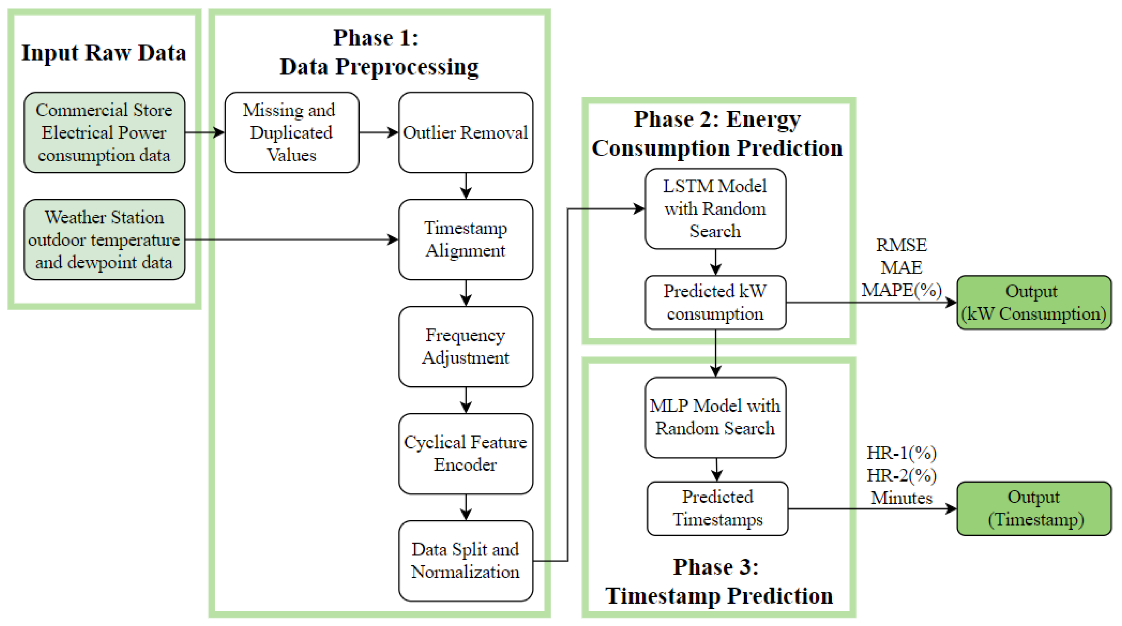
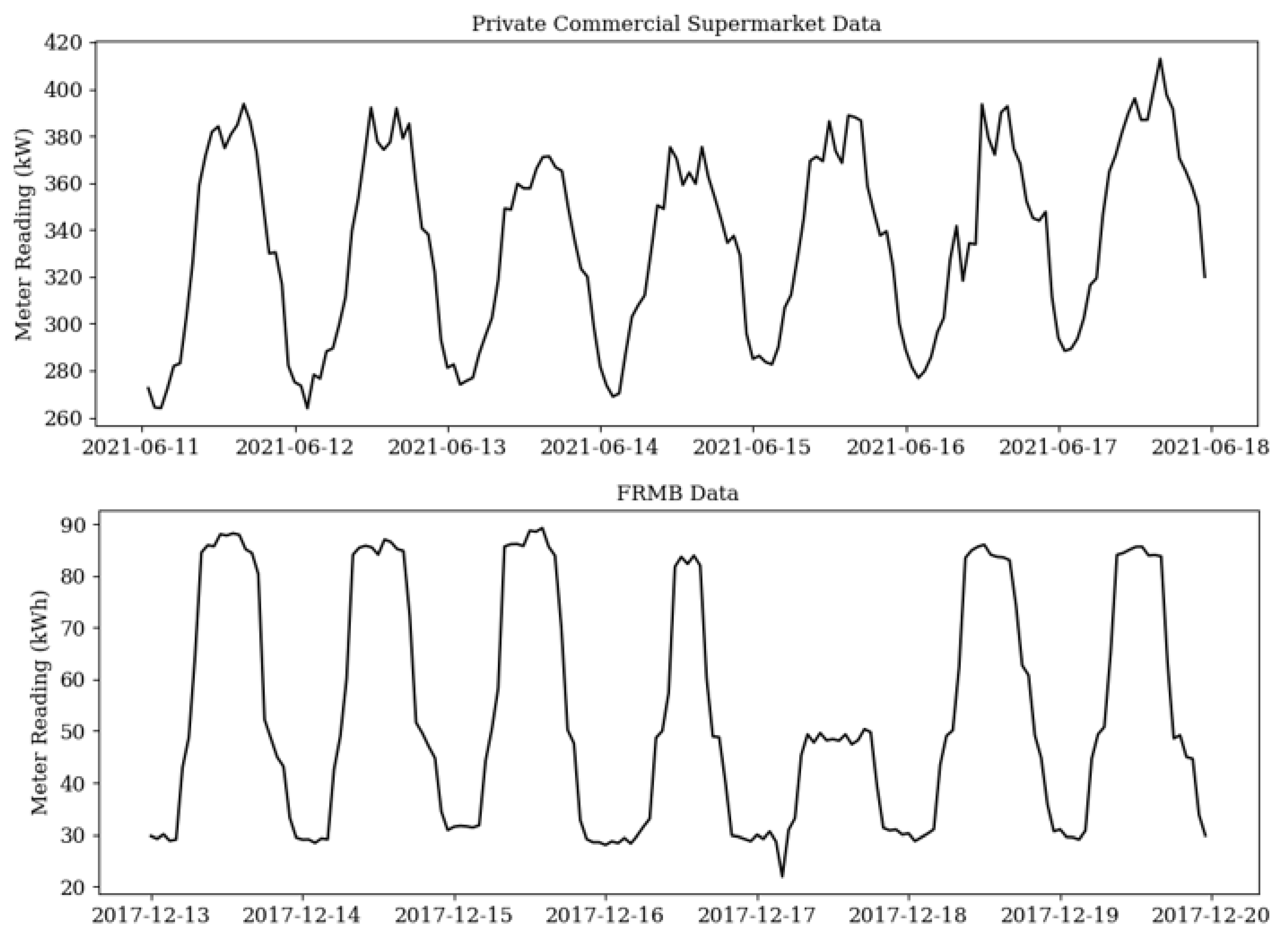
Figure 4 shows an overview of the proposed EPTP framework with three phases, namely data preprocessing, energy consumption prediction with the LSTM network, and timestamp prediction with the MLP model. The energy consumption raw data were obtained from the sensor reading in the commercial supermarket. Braun et al. [60] studied the energy consumption pattern in commercial supermarkets and concluded that half of the electricity usage in commercial supermarkets was directly related to the weather. Therefore, the outdoor temperature and dewpoint temperatures were extracted from the closest weather station as additional features. The raw data then underwent the data preprocessing steps to sanitize the input required for the deep learning model. Time-related variables were feature engineered as part of the input. In the second stage, the sanitized dataset passed through an LSTM model to predict the energy consumption of the commercial supermarket for the next 24 h. Finally, an MLP model was trained with the predicted 24-h energy consumption as the input to obtain the indices, which were compared to the real starting, peaking, and ending labels from the original dataset. As the end goal of the proposed EPTP framework, the prediction should not only contain the peak consumption value but also the indices for which it occurs 24 h in advance. The details regarding each step are described as follows.

4.1. Phase 1: Data Preprocessing

Impurities are naturally included in data collection when obtained from real-world applications. Data preprocessing serves as a necessary step to remove impurities in the dataset and improve accuracy and reliability in model training. Starting off, missing and duplicated values may occur during the data collection stage, caused by unexpected situations such as unstable sensor connections, data corruption, or hardware failures. In this EPTP framework, short-term missing datapoints were linearly interpolated with the average of the previous and next datapoints. The daily energy consumption data were removed for any day containing long-term missing data. A two-hour threshold was used to distinguish between short- and long-term missing values. Duplicated entries were simply removed to ensure that each timestamp contained only one datapoint.
In the data collection stage, observations are recorded based on the sensor reading. However, the sensor readings may contain noise, errors, or unwanted data due to potential sensor faults or connection issues [61]. These observations are considered outliers that should be removed to improve the data quality for better prediction accuracy. In the EPTP framework, the outliers in the commercial building energy consumption data are detected and replaced with the Hampel filter [62]. The Hampel filter is a type of decision-based filter that implements the moving window of the Hampel identifier [63] so that the sliding window length is 2 N + 1 , where N represents a positive integer called the window half-width. Equation (4) shows the detection and replacement of the outliers using the Hampel filter, where m k and ψ k represent the median and the median absolute deviations of the sliding window, respectively, and τ represents the threshold value. In the utilization of the Hampel filter, N and τ are user-defined parameters that can be adjusted based on the specific outlier detection and replacement requirements. Specifically, N controls the size of the sliding window that is used to calculate m k and ψ k , and τ determines the boundary, hence the number of outliers detected in the dataset. In this framework, N was chosen to be the number of datapoints per day; τ was chosen to have the default value of 3 based on Pearson’s rule [64].
y k = m k , i f x k m k > τ × ψ k , x k , i f x k m k τ × ψ k .
Since the energy consumption data of the commercial building and the weather information originate from distinct sources, both the timestamp and frequency need to be aligned. In the timestamp alignment, modifications included converting from Coordinated Universal Time to local time, and accommodating any daylight-saving time changes. In the conversion from Coordinated Universal Time to local time, the time zone was determined using the geological location of the commercial building. For the observations collected during the daylight-saving time changes, the data were treated as missing and duplicated values and sanitized using the interpolation and removal methods. In frequency adjustment, the data samples were either averaged to a lower frequency or interpolated to a higher frequency based on the prediction requirements.
In the final steps of data preprocessing, cyclical feature encoder and normalization were implemented to enhance the model performance. Electricity consumption in commercial building is affected by the hour of the day [20]. This is especially true in the retail industry, as the customer footprint increases during the store’s operating hours. Therefore, in this proposed EPTP framework, the hour of the day (i.e., ranges between 0 and 23) was included as an independent variable to predict energy consumption. A common method for encoding the cyclical feature is to transform the data into two dimensions with a trigonometric encoder. To ensure that each interval was uniquely represented, both sine and cosine transformations were included, as shown in Equation (5). The complete dataset was then split into training, validation, and test sets based on roughly a 70:15:15 ratio to normalize the data using the min–max scaling technique to transform the features into the same unit of measure as the raw attributes typically lack sufficient quality for obtaining accurate predictive models. Normalization aims to transform the original attributes to enhance the model’s predictive capability [65].
x s i n = s i n 2 π x m a x ( x ) x c o s = c o s 2 π x m a x ( x )

4.2. Phase 2: Predictor Model for Energy Consumption

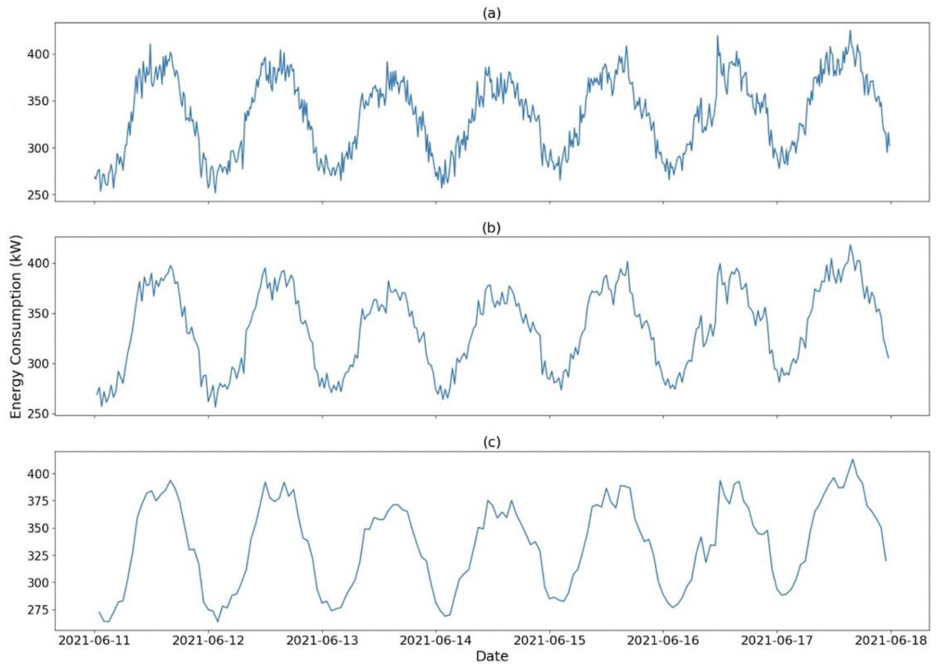
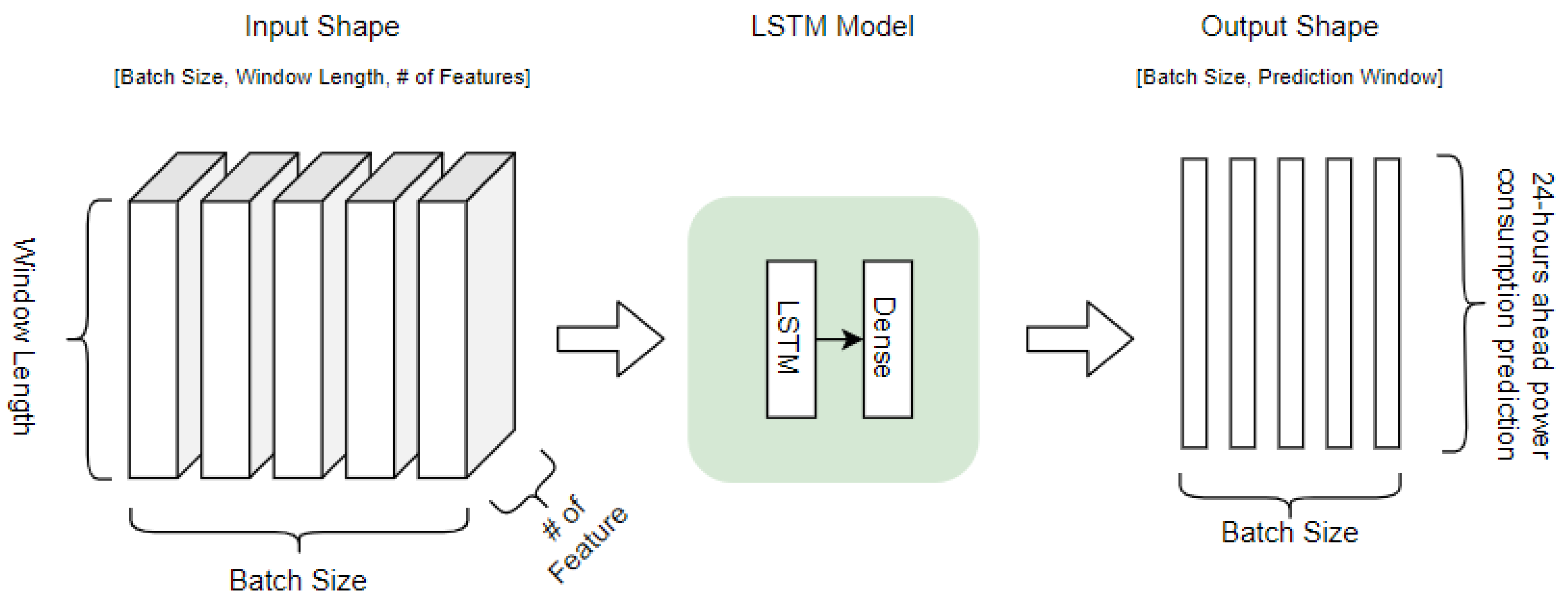
The second phase of the proposed EPTP framework was to predict energy consumption using the given features with LSTM modeling, as depicted in Figure 5. Input features included energy consumption (unit: kW), outdoor temperature (unit: °C), dewpoint temperature (unit: °C), and the transformed cyclical feature. The input layer of the LSTM modeling accepts 3-dimensional input in the shape of b a t c h   s i z e × w i n d o w   l e n g t h × f e a t u r e   c o u n t . Shuffling was rejected on the input features to maintain the relationship for time series sequential data.
However, the output of the LSTM model depends on the frequency at which the data are processed. The objective of this EPTP framework was not only to predict the amount of energy usage for the peak consumption, but also the corresponding timestamp. Hence, it was necessary to simultaneously generate the consumption for the next day. Therefore, the output shape for Phase 2 was b a t c h   s i z e × 24 , b a t c h   s i z e × 48 , b a t c h   s i z e × 96 for the 1-h, 30-min, and 15-min frequencies, respectively. The hyperparameters for the LSTM modeling included the sliding window length, activation function, number of LSTM layers, batch size, and learning rate. The random search algorithm was utilized for hyperparameter optimization as the search space included a combination of continuous and categorical variables. Random search optimization also aims to reduce computational power and resources as tuning is processed with five hyperparameters.
In this framework, the energy consumption predictions were evaluated against the MAE, RMSE, and MAPE. Equations (6)–(8) provide the formula for the calculations where t i and t i ^ represent the grounded truth and predicted values, respectively. Among all three metrics, MAPE provides a better understanding of the error scale, whereas RMSE and MAE are not normalized regarding the prediction scale. For MAPE, the higher the value, the better the result, while for the RMSE and MAE, the lower the value, the better the result.
R M S E = 1 m i = 1 m ( t i t i ^ ) 2
M A E = 1 m i = 1 m | t i t i ^ |
M A P E = 100 % m i = 1 m t i t i ^ t i

4.3. Phase 3: Peak Index Model for Timestamp Prediction

In the final phase of the EPTP framework, an MLP model was proposed to predict the timestamps of the daily starting, peaking, and ending indices. To train for the MLP network, three timestamps per day were designated as true labels, allowing for a comparison with the model prediction. In such labeling, the peak consumption was defined using the BM approach in the extreme value theory. BM consists of dividing the observation period into non-overlapping blocks of equal size and retrieving the maximum value within each block [66]. Consider the total number of observations as P , which can be divided into B blocks of size M so that P = B × M . Equation (9) shows the retrieval of the peak value where X j ~ represents all the datapoints in block b and X b represents the corresponding peak value in the same block.
X b = max ( b 1 ) M < j bM X j ~
After defining the peak consumption, the main contribution of this study was to label the starting, peaking, and ending indices in each block b . The peaking index is defined as the timestamp so that the maximum energy consumption has occurred in the predefined window. In the EPTP framework, the window was defined to be 24 h so that M = 24 ,   48 ,   a n d   96 for the 1-h, 30-min, and 15-min resolutions, respectively. The starting index was extracted using the base value on the left-hand side of the peak. The peak occurrence was led by an increasing trend where the start timestamp of the increment was defined as the starting index of the peak. Similarly, the ending index was defined using the base value on the right-hand side. In addition, the duration of the peak was also validated so that a long period of peak occurrence was avoided, especially for the low-frequency data. This proposed EPTP framework used a four-hour threshold to validate the peak duration. If the peak duration lasts more than four hours based on the previous steps, the ending index will be updated if the consumption at the ending index is lower than that of the starting index. Likewise, the starting index will be adjusted if the consumption at the starting index is lower than that of the ending index. The justification ensures the duration between the starting and peaking indices was equal to the duration between the peaking and ending indices. This modification preserves the shape of the peak consumption while preventing excessively long peak durations, especially for low-frequency data. Once the true labels are extracted, these indices will be compared to the MLP model’s output for performance evaluation.
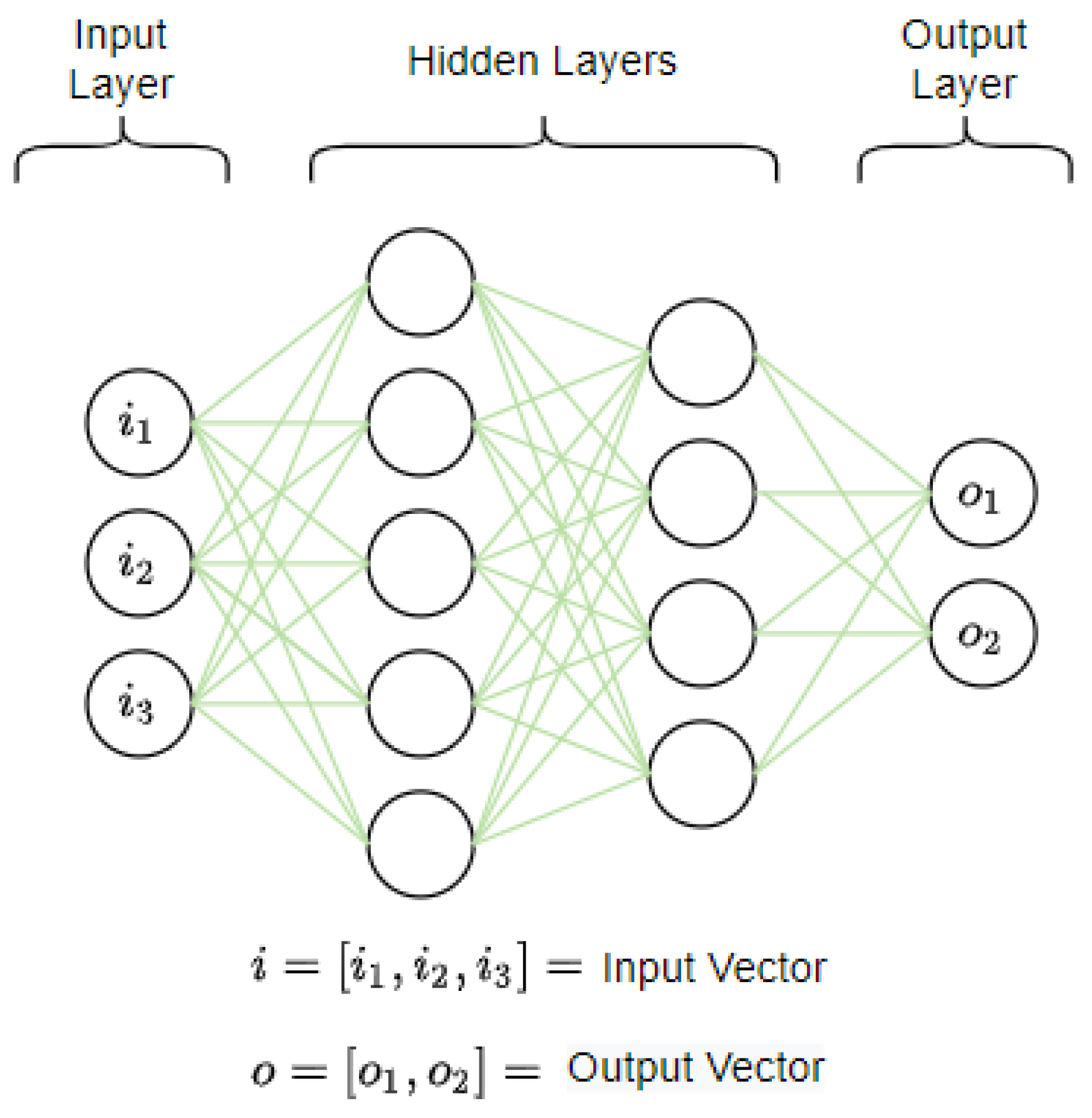
As mentioned, MLP models have successfully detected delays and time deviations for flight and traffic control applications. In this proposed EPTP framework, the MLP input layer accepts a 2-dimensional input in the shape of d a y   c o u n t × u n i t . Since the model was designed to predict the daily peak indices, the input needs to encompass the consumption data for the entire day. Consequently, depending on the prediction frequency, the input shape for the final phase of the EPTP framework was presented as d a y   c o u n t × 24 , d a y   c o u n t × 48 , and d a y   c o u n t × 96  with respect to the 1-h, 30-min, and 15-min frequencies, respectively. Shuffling was introduced at this stage as each day was treated as a standalone sample.
The output of the MLP model was d a y   c o u n t × 3 , as each neuron represents a single index. In the proposed EPTP framework, the starting, peaking, and ending indices need to be predicted for upcoming peak-shaving strategies in commercial building applications. As a consequence, the output layer contained three neurons. As previously mentioned, the predicted index was then compared with the day ahead labels to identify the model performance. The hyperparameters in this phase included the number of hidden layers and neurons on each layer, activation function, and learning rate. As the MLP model predicts the timestamps on a daily frequency (i.e., contains only 365 samples per year) and MLP is less computationally heavy compared to LSTM modeling, batching was not required in this phase.
The timestamp prediction was evaluated using the hit rate (HR) metric [67] and mean absolute minute deviation. Equation (10) shows the calculation of the HR metric, where δ represents the tolerance residual for the expected timestamp and h is a flag representing whether the predicted timestamp is within the tolerance interval. In this study, the tolerance interval was chosen to be one hour (HR-1) and two hours (HR-2) for a better comparison. This means that δ was {1, 2}, {2, 4}, and {4, 8} for the 1-h, 30-min, and 15-min resolutions, respectively. The higher the HR value, the better the results. Equation (11) shows the calculation for translating the timestamp MAE error into minute deviations for consistency as the model works with different resolutions.
H R = 100 % m i = 1 m h i     w h e r e     h i = 1 , t i ^ t i δ , t i + δ 0 ,   o t h e r w i s e .
M e a n   A b s o l u t e   M i n u t e   d e v i a t i o n = M A E × 15     f o r     15 m i n u t e   r e s o l u t i o n M A E × 30     f o r     30 m i n u t e   r e s o l u t i o n M A E × 60     f o r     1 h o u r   r e s o l u t i o n

5. Evaluation of the EPTP Framework

This section provides a comprehensive evaluation of the EPTP framework. The section begins with the evaluation setup and metrics, followed by experiments conducted on two real-world datasets with a detailed discussion of the findings.

5.1. Evaluation Setup

The models and experiments ran on a Linux server with an Intel® Core™ i7-6850K Processor and 64 GB RAM, with 2 GPUs GeForce GTX 1080 Ti and OS Ubuntu 20.4. The algorithm and framework were implemented in Python version 3.9.0. The deep learning models in the case study were implemented using the PyTorch library with Ray tune hyperparameter optimization. Table 1 shows the hyperparameters and their search spaces for the LSTM modeling. The sliding window considers the weekly patterns of the energy consumption data with lower and higher sensitivity. To generalize the results, Ray tune optimization was performed with 20 trials. Since random search was used as the optimization method with the learning rate as a continuous hyperparameter, regenerating the searching process with the exact learning rate using seeding was impossible. Therefore, the top three trials with the highest accuracy were repeated for the second time to generate the averaged results. With the best energy consumption prediction results, the model moves to the third phase of predicting the timestamps. Table 2 lists the hyperparameters and their search spaces for the MLP modeling. Since the input layer consisted of the predicted daily energy consumption data and the output layer contained three neurons, one for each timestamp, the neuron size per hidden layer was chosen to provide a linear division between the neurons of the input and the output layers. The MLP hyperparameter optimization process was also performed with 20 trials, with the top three trials repeated for a second time to generate the average results.

5.2. Evaluation with a Real-World Commercial Supermarket Dataset

The private commercial dataset was collected from a supermarket located in Quebec, Canada. The store opens seven days a week from 8:00 a.m. to 10:00 p.m. (excluding national holidays) and offers a variety of products and services including in-house bakeries, fish and seafood departments, pastry-shop counters, and bistro express. The available data ranged from 17 August 2020 to 24 January 2023, for a duration of 890 days. The electricity consumption data were collected with a resolution of one datapoint per minute. The weather information was extracted from the closest station listed on the Environment Canada website at a frequency of 1 datapoint per hour. Three cases were created to evaluate the model performance, specifically at a 1-h resolution, 30-min resolution, and 15-min resolution. Figure 6 provides an example of the weekly energy consumption pattern in which a higher resolution figure contains more details and spikiness. As the resolution decreases, the figure shows a smoother trend with less information. With data splitting in the proportions 70:15:15, the training set contained 620 days of information, and validation and test sets each contained 135 days of information.

5.2.1. Performance Baselines

In this experiment, two performance baselines were established for a later comparison with the results of the proposed EPTP framework. The first baseline was created so that the energy consumption prediction was based on SVR, followed by MLP for the timestamp predictions. The raw data underwent the three phases outlined in Section 4, except that the energy consumption prediction was performed with SVR instead of LSTM architecture. Table 3 outlines the hyperparameters for the SVR model. The energy consumption predictions with the highest accuracy were then grouped into days based on the number of datapoints (i.e., 24, 48, and 96 datapoints for the 1-h, 30-min, and 15-min resolutions, respectively). The grouped data then underwent the MLP model for timestamp prediction of the starting, peaking, and ending indices.
The second baseline was created so that the peak index for the commercial building application was extracted using the common method of BM with extreme value theory. This means that instead of modeling for the indices, the timestamp for the highest energy consumption for each day was treated as the peak index. However, since the model was not trained to learn the starting and ending indices in the second baseline, only the peak index was compared to the proposed EPTP framework in the later experiments. Table 4 summarizes the results of the two baseline models to compare the timestamp indices. The results of the proposed EPTP framework were compared to the HR-1, HR-2, and minute deviations to validate its performance.

5.2.2. EPTP Performance on the Private Dataset

The model was initially proposed to work with 15-min resolutions based on the industrial specifications. However, when high-frequency data are inaccessible, predictions using lower-frequency data is deemed necessary. Therefore, three cases were used to evaluate the model performance, specifically the 1-h, 30-min, and 15-min resolutions. The raw data were then preprocessed so that the high-frequency data were averaged into the expected resolution, and the low-frequency data were interpolated if necessary. The LSTM network was optimized with 20 trials so that the best hyperparameters were used to retrieve the energy prediction, thereafter, the index predictions were also optimized with 20 trials using the MLP network.
The training time for each LSTM random search trial was around 0.52 h, 2.45 h, and 5.33 h for the 1-h, 30-min, and 15-min resolutions, respectively. The MLP training time was negligent since the MLP model requires fewer training resources for predicting timestamps on a daily frequency (i.e., contains only 365 samples per year). Table 5 summarizes the results of the LSTM modeling and shows that the MAPE error on the energy consumption was comparable across different resolutions, at around 4.5%. Table 6 shows the metrics in evaluating the predicted timestamps and concludes that the predictive results presented a better accuracy as the input data frequency increased (i.e., more samples per hour).

5.2.3. Results and Discussions of the Commercial Supermarket Dataset

Figure 7 presents the boxplot of the differences between the predicted indices and the real indices in all three resolutions using the EPTP framework. It shows that the range between the first and third quartiles was narrower for the higher resolution data. However, the boxplot of the 15-min resolution data showed some outliers in the prediction. Upon further examination of Figure 8, Figure 9 and Figure 10, which show the comparison between the density plot of different resolutions with the EPTP framework, they revealed that the predicted results better captured the bi-modal distribution in the real label as the frequency of data increased. This prediction of the bi-modal timestamp label may have contributed to the outliers in the boxplot for the higher frequency input. The discrepancy between the unimodal prediction and the bi-modal true labels indicates that the model emphasizes a single dominant pattern in the output, potentially due to the lack of input features. Future work on this study should consider including the occupancy, customer footprint, or detailed operational schedules to further improve the timestamp predictions in low-frequency data.
The EPTP framework also generated better results when compared to the performance baselines, especially for the 15-min resolution data. The LSTM modeling outperformed the SVR modeling in following the trends and fluctuations in the commercial supermarket consumption data, resulting in better timestamp prediction results. The EPTP framework also generated an HR-2 of 86% with 62-min deviations for the peak indices using 15-min resolution data, compared to 65% with 120-min deviations in the second performance baseline. Although the second baseline of using BM provided a higher HR for the 30-min resolution, it lacked insights into the starting and ending indices. While the EPTP framework still needs to be further improved with more granular data frequency, it is still recommended for providing insights into the duration of the peak period.

5.3. Evaluation with the Benchmark Dataset

The benchmark dataset was retrieved from the Building Data Genome Project 2 (BDG2) open-sourced data [68,69]. BDG2 contains 1636 non-residential buildings with a range of two full years (2016–2017) at an hourly frequency, in which only twelve are categorized into “Retail” for primary use type. For the purpose of benchmarking, the Fox Retail Manie Building (FRMB) was chosen to model the peak values and timestamps. Figure 11 shows an example of the weekly energy consumption for six out of twelve “Retail” buildings in the BDG2 dataset. Upon close inspection, the FRMB had better data quality than the other retail buildings. FRMB also has the highest correlation, at 0.56, with the private dataset that was previously introduced. All other retail buildings from BDG2 had a correlation of below 0.47 with the private dataset. With data splitting in the proportions 70:15:15, the training set contained 560 days of information, and the validation and test sets each contained 85 days of information. As all of the data were provided at an hourly resolution, the benchmark dataset was only used to model the low-frequency application.

5.3.1. EPTP Performance on the Benchmark Dataset

The FRMB consumption data underwent the same procedure as the private commercial supermarket dataset. However, since the BDG2 dataset contained two years of data at an hourly resolution, only hourly modeling was performed to avoid excessive data interpolation. The same search space was used for both the energy consumption predictions and timestamp predictions to maintain consistency. Similarly, the LSTM network was optimized with 20 trials so that the best hyperparameters were used to retrieve the energy prediction. Thereafter, the index predictions were also optimized with 20 trials using the MLP network. Table 7 summarizes the results of the LSTM modeling of FRMB in comparison to the private commercial supermarket dataset that was previously discussed. Table 8 shows the timestamp predictions with MLP modeling compared with the commercial supermarket results.

5.3.2. Results and Discussions of the Benchmark Dataset

In the energy consumption predictions, as seen in Table 7, the RMSE and MAE errors for FRMB were lower, and the MAPE error was high. Further examination concluded that this was mainly attributed to two factors. First, the range of meter reading for FRMB was on a lower scale compared to the private commercial supermarket dataset. The highest reading from FRMB was around 118 kWh, whereas the highest reading from the private commercial supermarket dataset was around 532 kW. Although the two datasets consisted of different units, the value remained the same as the prediction was based on an hourly resolution. Second, the commercial supermarket and the FRMB had different operating schedules, as seen in Figure 12. It appears that the building is not in full operation seven days a week as the consumption was substantially lower on some days than others for the FRMB. In contrast, the commercial supermarket opens seven days a week (excluding national holidays). This implies that the variation in energy consumption for the private dataset was minimal. Since the details of the operating schedule was not disclosed with the dataset, it is difficult to generate a model result as good as that of the commercial supermarket.
The proposed EPTP framework resulted in a deviation of 128 min on the peak index for FRMB and 148 min for the commercial building using the hourly resolution. Even though the energy consumption prediction for FRMB deviated from the actual consumption, the daily trend remained similar. In addition, Figure 13 shows that the real indices for FRMB had a unimodal distribution compared to the bimodal distribution in the private commercial supermarket dataset. This feature made the model easier to train, thus improving the HR metrics.

6. Conclusions

This paper proposed a three-phase EPTP framework designed to identify the energy peaks and precisely predict the timestamps associated with their occurrences. In the initial phase, energy consumption data and weather information were obtained and sanitized for the deep learning model. The sanitized data then passed through the second phase with LSTM modeling to predict the day-ahead energy consumption. Finally, the predicted day-ahead energy consumption was input to the MLP model to generate timestamps as the output. The performance of the MLP model was evaluated using peak occurrence labels derived from real data. The proposed EPTP framework was evaluated with two datasets: a private commercial supermarket and established open-source low-frequency data. The results show that the EPTP framework exhibited a superior performance with higher frequency data. When compared to the performance baselines, the HR-2 improved from 65.3% to 86%, and the minute deviation decreased from 120 min to 62 min for the 15-min resolution. Finally, the EPTP framework was trained with an open-source retail building. Despite FRMB being susceptible to fluctuations arising from varied operational patterns, the predictions of the index values yielded comparable accuracy to those of the private dataset with the same frequency. This experiment concludes that the unimodal distribution of the real peaks will result in a higher HR compared to the bimodal distribution.
Further research will focus on enhancing the framework accuracy for low-resolution data and providing additional validation. The proposed EPTP framework was initially established to operate with high-resolution data, specifically 15-min intervals. However, its performance degrades when applied to lower resolutions such as 1-h intervals. Hence, areas of improvement should focus on improving the accuracy of the index prediction in low-resolution data. During the benchmarking process of using open-sourced datasets, the proposed EPTP framework revealed potential improvements in energy consumption prediction, especially in accommodating varied operating patterns. In addition, the framework should be examined to validate whether incorporating historical peak information and store operation features such as occupancy and production could enhance the accuracy of the timestamp prediction results. Finally, further research efforts should concentrate on applying the model in real-time with Edge devices, aiming to enhance accessibility and applicability.

Author Contributions

Methodology, M.Z., S.G.-R., H.N. and C.Z.; software, M.Z.; validation, M.Z., S.G.-R. and H.N.; formal analysis, M.Z.; investigation, M.Z., S.G.-R., H.N. and C.Z.; writing—original draft preparation, M.Z.; writing—review and editing, S.G.-R., H.N., M.A.M.C. and A.S.; visualization, M.Z.; supervision, M.A.M.C. and A.S.; project administration, C.Z.; funding acquisition, C.Z. and A.S. All authors have read and agreed to the published version of the manuscript.

Funding

The proposed research was funded by Mitacs Accelerate Grant and the Neelands Group.

Data Availability Statement

The raw data supporting the conclusions of this article will be made available by the authors on request.

Conflicts of Interest

Authors Hooman Nouraei and Craig Zych were employed by the company Neelands Group Ltd. The remaining authors declare that the research was conducted in the absence of any commercial or financial relationships that could be construed as a potential conflict of interest.

Abbreviations

BDG2Building Data Genome Project 2
BMBlock maxima
EPTPEnergy Peaks and Timestamping Prediction
FRMBFox Retail Manie Building
HRHit rate
LSTMLong short-term memory
MAEMean absolute error
MAPEMean absolute percentage error
MLPMultilayer perceptron
RMSERoot mean squared error
RNNRecurrent neural network
SVRSupport vector regression

References

  1. Wan, K.K.W.; Li, D.H.W.; Pan, W.; Lam, J.C. Impact of climate change on building energy use in different climate zones and mitigation and adaptation implications. Appl. Energy 2012, 97, 274–282. [Google Scholar] [CrossRef]
  2. Santamouris, M. Innovating to zero the building sector in Europe: Minimising the energy consumption, eradication of the energy poverty and mitigating the local climate change. Sol. Energy 2016, 128, 61–94. [Google Scholar] [CrossRef]
  3. Berardi, U. A cross-country comparison of the building energy consumptions and their trends. Resour. Conserv. Recycl. 2017, 123, 230–241. [Google Scholar] [CrossRef]
  4. IEA. Buildings; Technical Report; IEA: Paris, France, 2022.
  5. Global Alliance for Buildings and Construction. 2020 Global Status Report for Buildings and Construction; Global Alliance for Buildings and Construction: Paris, France, 2020. [Google Scholar]
  6. Allouhi, A.; El Fouih, Y.; Kousksou, T.; Jamil, A.; Zeraouli, Y.; Mourad, Y. Energy consumption and efficiency in buildings: Current status and future trends. J. Clean. Prod. 2015, 109, 118–130. [Google Scholar] [CrossRef]
  7. Lam, J.C.; Wan, K.K.W.; Tsang, C.L.; Yang, L. Building energy efficiency in different climates. Energy Convers. Manag. 2008, 49, 2354–2366. [Google Scholar] [CrossRef]
  8. Pérez-Lombard, L.; Ortiz, J.; Pout, C. A review on buildings energy consumption information. Energy Build. 2008, 40, 394–398. [Google Scholar] [CrossRef]
  9. Mahjoub, S.; Chrifi-Alaoui, L.; Marhic, B.; Delahoche, L. Predicting Energy Consumption Using LSTM, Multi-Layer GRU and Drop-GRU Neural Networks. Sensors 2022, 22, 4062. [Google Scholar] [CrossRef]
  10. Yan, K.; Wang, X.; Du, Y.; Jin, N.; Huang, H.; Zhou, H. Multi-step short-term power consumption forecasting with a hybrid deep learning strategy. Energies, 2018; 11, 3089. [Google Scholar]
  11. Elsaraiti, M.; Ali, G.; Musbah, H.; Merabet, A.; Little, T. Time Series Analysis of Electricity Consumption Forecasting Using ARIMA Model. In Proceedings of the 2021 IEEE Green Technologies Conference (GreenTech), Denver, CO, USA, 7–9 April 2021. [Google Scholar]
  12. Amjady, N. Short-term hourly load forecasting using time-series modeling with peak load estimation capability. IEEE Trans. Power Syst. 2001, 16, 798–805. [Google Scholar] [CrossRef]
  13. Taieb, S.B.; Taylor, J.W.; Hyndman, R.J. Hierarchical Probabilistic Forecasting of Electricity Demand with Smart Meter Data. J. Am. Stat. Assoc. 2021, 116, 27–43. [Google Scholar] [CrossRef]
  14. U.S. Energy Information Administration. 2018 Commercial Buildings Energy Consumption Survey Consumption and Expenditures Highlights; U.S. Energy Information Administration: Washington, DC, USA, 2018.
  15. U.S. Energy Information Administration. 2018 Commercial Buildings Energy Consumption Survey Building Characteristics Highlights; U.S. Energy Information Administration: Washington, DC, USA, 2018.
  16. Tassou, S.A.; Ge, Y.; Hadawey, A.; Marriott, D. Energy consumption and conservation in food retailing. Appl. Therm. Eng. 2011, 31, 147. [Google Scholar] [CrossRef]
  17. Timma, L.; Skudritis, R.; Blumberga, D. Benchmarking Analysis of Energy Consumption in Supermarkets. Energy Procedia 2016, 95, 435–438. [Google Scholar] [CrossRef]
  18. Glavan, M.; Gradišar, D.; Moscariello, S.; Juričić, Đ.; Vrančić, D. Demand-side improvement of short-term load forecasting using a proactive load management–a supermarket use case. Energy Build. 2019, 186, 186–194. [Google Scholar] [CrossRef]
  19. Mocanu, E.; Nguyen, P.H.; Gibescu, M.; Kling, W.L. Deep learning for estimating building energy consumption. Sustain. Energy Grids Netw. 2016, 6, 91–99. [Google Scholar] [CrossRef]
  20. Yildiz, B.; Bilbao, J.I.; Sproul, A.B. A review and analysis of regression and machine learning models on commercial building electricity load forecasting. Renew. Sustain. Energy Rev. 2017, 73, 1104–1122. [Google Scholar] [CrossRef]
  21. Nti, I.K.; Teimeh, M.; Nyarko-Boateng, O.; Adekoya, A.F. Electricity load forecasting: A systematic review. J. Electr. Syst. Inf. Technol. 2020, 7, 13. [Google Scholar] [CrossRef]
  22. Nepal, B.; Yamaha, M.; Yokoe, A.; Yamaji, T. Electricity load forecasting using clustering and ARIMA model for energy management in buildings. Jpn. Archit. Rev. 2020, 3, 62–76. [Google Scholar] [CrossRef]
  23. Guo, N.; Chen, W.; Wang, M.; Tian, Z.; Jin, H. Appling an Improved Method Based on ARIMA Model to Predict the Short-Term Electricity Consumption Transmitted by the Internet of Things (IoT). Wirel. Commun. Mob. Comput. 2021, 2021, 6610273. [Google Scholar] [CrossRef]
  24. Hong, W.; Fan, G. Hybrid Empirical Mode Decomposition with Support Vector Regression Model for Short Term Load Forecasting. Energies 2019, 12, 1093. [Google Scholar] [CrossRef]
  25. Fan, G.; Peng, L.; Zhao, X.; Hong, W. Applications of Hybrid EMD with PSO and GA for an SVR-Based Load Forecasting Model. Energies 2017, 10, 1713. [Google Scholar] [CrossRef]
  26. Zhang, F.; Deb, C.; Lee, S.E.; Yang, J.; Shah, K.W. Time series forecasting for building energy consumption using weighted Support Vector Regression with differential evolution optimization technique. Energy Build. 2016, 126, 94–103. [Google Scholar] [CrossRef]
  27. Jang, J.; Han, J.; Leigh, S.B. Prediction of heating energy consumption with operation pattern variables for non-residential buildings using lstm networks. Energy Build. 2022, 255, 111647. [Google Scholar] [CrossRef]
  28. Pallonetto, F.; Jin, C.; Mangina, E. Forecast electricity demand in commercial building with machine learning models to enable demand response programs. Energy AI 2022, 7, 100121. [Google Scholar] [CrossRef]
  29. Fu, H.; Baltazar, J.; Claridge, D.E. Review of developments in whole-building statistical energy consumption models for commercial buildings. Renew. Sustain. Energy Rev. 2021, 147, 111248. [Google Scholar] [CrossRef]
  30. Ai, S.; Chakravorty, A.; Rong, C. Evolutionary Ensemble LSTM based Household Peak Demand Prediction. In Proceedings of the 2019 International Conference on Artificial Intelligence in Information and Communication (ICAIIC), Okinawa, Japan, 11–13 February 2019. [Google Scholar]
  31. Aouad, M.; Hajj, H.; Shaban, K.; Jabr, R.A.; El-Hajj, W. A CNN-Sequence-to-Sequence network with attention for residential short-term load forecasting. Electr. Power Syst. Res. 2022, 211, 108152. [Google Scholar] [CrossRef]
  32. Satre-Meloy, A.; Diakonova, M.; Grünewald, P. Cluster analysis and prediction of residential peak demand profiles using occupant activity data. Appl. Energy 2020, 260, 114246. [Google Scholar] [CrossRef]
  33. Ibrahim, I.A.; Hossain, M.J. LSTM neural network model for ultra-short-term distribution zone substation peak demand prediction. In Proceedings of the 2020 IEEE Power & Energy Society General Meeting (PESGM), Montreal, QC, Canada, 2–6 August 2020. [Google Scholar]
  34. Lu, H.; Cheng, F.; Ma, X.; Hu, G. Short-term prediction of building energy consumption employing an improved extreme gradient boosting model: A case study of an intake tower. Energy 2020, 203, 117756. [Google Scholar] [CrossRef]
  35. Mughees, N.; Mohsin, S.A.; Mughees, A.; Mughees, A. Deep sequence to sequence Bi-LSTM neural networks for day-ahead peak load forecasting. Expert Syst. Appl. 2021, 175, 114844. [Google Scholar] [CrossRef]
  36. Amara-Ouali, Y.; Fasiolo, M.; Goude, Y.; Yan, H. Daily peak electrical load forecasting with a multi-resolution approach. Int. J. Forecast. 2023, 39, 1272–1286. [Google Scholar] [CrossRef]
  37. Lebotsa, M.E.; Sigauke, C.; Bere, A.; Fildes, R.; Boylan, J.E. Short term electricity demand forecasting using partially linear additive quantile regression with an application to the unit commitment problem. Appl. Energy 2018, 222, 104–118. [Google Scholar] [CrossRef]
  38. Boano-Danquah, J.; Sigauke, C.; Kyei, K. Analysis of Extreme Peak Loads Using Point Processes: An Application Using South African Data. IEEE Access 2020, 8, 2169–3536. [Google Scholar] [CrossRef]
  39. Fan, C.; Xiao, F.; Wang, S. Development of prediction models for next-day building energy consumption and peak power demand using data mining techniques. Appl. Energy 2014, 127, 1–10. [Google Scholar] [CrossRef]
  40. Taheri, S.; Razban, A. A novel probabilistic regression model for electrical peak demand estimate of commercial and manufacturing buildings. Sustain. Cities Soc. 2022, 77, 103544. [Google Scholar] [CrossRef]
  41. Chae, Y.T.; Horesh, R.; Hwang, Y.; Lee, Y.M. Artificial neural network model for forecasting sub-hourly electricity usage in commercial buildings. Energy Build. 2016, 111, 184–194. [Google Scholar] [CrossRef]
  42. Gilbert, C.; Browell, J.; Stephen, B. Probabilistic load forecasting for the low voltage network: Forecast fusion and daily peaks. Sustain. Energy Grids Netw. 2023, 34, 100998. [Google Scholar] [CrossRef]
  43. Soman, A.; Trivedi, A.; Irwin, D.; Kosanovic, B.; McDaniel, B.; Shenoy, P. Peak Forecasting for Battery-Based Energy Optimizations in Campus Microgrids. In Proceedings of the Eleventh ACM International Conference on Future Energy Systems, Virtual Event, Australia, 22–26 June 2020. [Google Scholar]
  44. Gardner, M.W.; Dorling, S. Artificial neural networks (the multilayer perceptron)—A review of applications in the atmospheric sciences. Atmos. Environ. 1998, 32, 2627–2636. [Google Scholar] [CrossRef]
  45. Jiang, Y.; Liu, Y.; Liu, D.; Song, H. Applying Machine Learning to Aviation Big Data for Flight Delay Prediction. In Proceedings of the 2020 IEEE Intl Conf on Dependable, Autonomic and Secure Computing, Intl Conf on Pervasive Intelligence and Computing, Intl Conf on Cloud and Big Data Computing, Intl Conf on Cyber Science and Technology Congress (DASC/PiCom/CBDCom/CyberSciTech), Calgary, AB, Canada, 17–22 August 2020. [Google Scholar]
  46. Alla, H.; Moumoun, L.; Balouki, Y. A Multilayer Perceptron Neural Network with Selective-Data Training for Flight Arrival Delay Prediction. Hindawi Sci. Program. 2021, 2021, 5558918. [Google Scholar] [CrossRef]
  47. Sherstinsky, A. Fundamentals of Recurrent Neural Network (RNN) and Long Short-Term Memory (LSTM) network. Phys. D Nonlinear Phenom. 2020, 404, 132306. [Google Scholar] [CrossRef]
  48. Hochreiter, S.; Schmidhuber, J. Long Short-Term Memory. Neural Comput. 1997, 9, 212. [Google Scholar] [CrossRef]
  49. Soutner, D.; Muller, L. Application of LSTM neural networks in language modelling. Int. Conf. Text Speech Dialogue 2013, 8082, 105–112. [Google Scholar]
  50. Li, D.; Qian, J. Text sentiment analysis based on long short-term memory. In Proceedings of the 2016 First IEEE International Conference on Computer Communication and the Internet (ICCCI), Wuhan, China, 13–15 October 2016. [Google Scholar]
  51. Cao, J.; Li, Z.; Li, J. Financial time series forecasting model based on ceemdan and lstm. Phys. A Stat. Mech. Its Appl. 2019, 519, 127–139. [Google Scholar] [CrossRef]
  52. Chimmula, V.K.R.; Zhang, L. Time series forecasting of covid-19 transmission in Canada using lstm networks. Chaos Solitons Fractals 2020, 135, 109864. [Google Scholar] [CrossRef]
  53. Feurer, M.; Hutter, F. Hyperparameter optimization in automated machine learning. In The Springer Series on Challenges in Machine Learning; Springer: Berlin/Heidelberg, Germany, 2019. [Google Scholar]
  54. Heaton, J. Introduction to Neural Networks with Java, 2nd ed.; Heaton Research, Inc.: Chesterfield, MI, USA, 2008; p. 158. [Google Scholar]
  55. Sharma, S.; Sharma, S.; Athaiya, A. Activation functions in neural networks. Int. J. Eng. Appl. Sci. Technol. 2020, 4, 310–316. [Google Scholar] [CrossRef]
  56. Kuhn, M.; Johnson, K. Applied Predictive Modeling; Springer: Berlin/Heidelberg, Germany, 2013. [Google Scholar]
  57. Montgomery, D. Design and Analysis of Experiments, 8th ed.; John Wiley & Sons, Inc.: Hoboken, NJ, USA, 2013; Chapter 5. [Google Scholar]
  58. Bergstra, J.; Bengio, Y. Random search for hyper-parameter optimization. J. Mach. Learn. Res. 2012, 13, 281–305. [Google Scholar]
  59. Shahriari, B.; Swersky, K.; Wang, Z.; Adams, R.P.; De Freitas, N. Taking the human out of the loop: A review of Bayesian optimization. Proc. IEEE 2015, 104, 148–175. [Google Scholar] [CrossRef]
  60. Braun, M.R.; Altan, H.; Beck, S.B.M. Using regression analysis to predict the future energy consumption of a supermarket in the UK. Appl. Energy 2014, 130, 305–313. [Google Scholar] [CrossRef]
  61. Blázquez-García, A.; Conde, A.; Mori, U.; Lozano, J.A. A Review on Outlier/Anomaly Detection in Time Series Data. ACM Comput. Surv. 2021, 54, 1–33. [Google Scholar] [CrossRef]
  62. Pearson, R.; Neuvo, Y.; Astola, J.; Gabbouj, M. Generalized Hampel Filters. EURASIP J. Adv. Signal Process 2016, 2016, 87. [Google Scholar] [CrossRef]
  63. Davies, L.; Gather, U. The Identification of Multiple Outliers. J. Am. Stat. Assoc. 1993, 88, 797–801. [Google Scholar] [CrossRef]
  64. Pearson, R.K. Outliers in process modeling and identification. IEEE Trans. Control Syst. Technol. 2002, 10, 55–63. [Google Scholar] [CrossRef]
  65. García, S.; Luengo, J.; Herrera, F. Data Preprocessing in Data Mining: Data Preparation Basic Models; Springer International Publishing: Berlin/Heidelberg, Germany, 2015. [Google Scholar]
  66. Ferreira, A.; Haan, L. On the block maxima method in extreme value theory: PWM estimators. Ann. Stat. 2013, 43, 276–298. [Google Scholar] [CrossRef]
  67. Xue, J.; Xu, Z.; Watada, J. Building an integrated hybrid model for short-term and mid-term load forecasting with genetic optimization. Int. J. Innov. Comput. Inf. Control 2012, 8, 7381–7391. [Google Scholar]
  68. Miller, C.; Kathirgamanathan, A.; Picchetti, B.; Arjunan, P.; Park, J.Y.; Nagy, Z.; Raftery, P.; Hobson, B.W.; Shi, Z.; Meggers, F. The building data genome project 2: Energy meter data from the ashrae great energy predictor iii competition. Sci. Data 2020, 7, 368. [Google Scholar] [CrossRef]
  69. Miller, C.; Arjunan, P.; Kathirgamanathan, A.; Fu, C.; Roth, J.; Park, J.Y.; Balbach, C.; Gowri, K.; Nagy, Z.; Fontanini, A.D.; et al. The ashrae great energy predictor iii competition: Overview and results. Sci. Technol. Built Environ. 2020, 26, 1427–1447. [Google Scholar] [CrossRef]
Figure 1. An MLP model with two hidden layers.
Energies 17 01672 g001
Figure 2. Internal structure of an artificial neuron.
Energies 17 01672 g002
Figure 3. Internal structure of an LSTM unit.
Energies 17 01672 g003
Figure 4. The proposed EPTP framework.
Energies 17 01672 g004
Figure 5. Input and output shapes of the LSTM model.
Energies 17 01672 g005
Figure 6. Sample weekly energy consumption data for the private commercial supermarket dataset: (a) 15-min resolution, (b) 30-min resolution, (c) 1-h resolution.
Energies 17 01672 g006
Figure 7. Comparison of the boxplot in predicting the starting, peaking, and ending indices with MLP modeling: (a) 15-min resolution, (b) 30-min resolution, (c) 1-h resolution.
Energies 17 01672 g007
Figure 8. Comparison of the density plot on the test set between the real indices and predicted indices for the 15-min resolution: (a) starting index, (b) peaking index, (c) ending index.
Energies 17 01672 g008
Figure 9. Comparison of the density plot on the test set between the real indices and predicted indices for the 30-min resolution: (a) starting index, (b) peaking index, (c) ending index.
Energies 17 01672 g009
Figure 10. Comparison of the density plot on the test set between the real indices and predicted indices for the 1-h resolution: (a) starting index, (b) peaking index, (c) ending index.
Energies 17 01672 g010
Figure 11. Sample weekly electrical meter reading data for the BDG2 dataset with retail buildings as the primary use type.
Energies 17 01672 g011
Figure 12. Comparison of the meter reading in a weekly sample between the private commercial supermarket and FRMB.
Energies 17 01672 g012
Figure 13. Comparison of the density plot for the FRMB test set between the real and predicted indices on an hourly resolution: (a) starting index, (b) peaking index, (c) ending index.
Energies 17 01672 g013
Table 1. Phase 2—hyperparameters and search space for LSTM model training.
HyperparameterDescriptionSearch Space
Sliding window (SW)Historical window sizeSample * × {5, 7, 10}
ActivationThe activation function for each layer{tanh, ReLu, Sigmoid}
Learning rate (LR)Learning rate for the optimizerLog uniform {0.01, 0.0001}
Batch sizeNumber of samples processed before update{256, 512, 1024}
LSTM layerNumber of LSTM layers{1, 2}
* Sample: Number of datapoints per day. Sample = {24, 48, 96} for {1-h, 30-min, 15-min} resolutions.
Table 2. Phase 3—hyperparameters and search space for MLP model training.
HyperparameterDescriptionSearch Space
Hidden layerNumber of hidden layers{1, 2, 3} *
Neuron size 1The number of hidden neurons for the first layer Random   integer   { 18 , 23 }     f o r     1 h o u r { 34 , 47 }     f o r     30 m i n u t e { 66 , 95 }     f o r     15 m i n u t e
Neuron size 2The number of hidden neurons for the second layer Random   integer   { 11 , 17 }     f o r     1 h o u r { 19 , 33 }     f o r     30 m i n u t e { 35 , 65 }     f o r     15 m i n u t e
Neuron size 3The number of hidden neurons for the third layer Random   integer   { 4 , 10 }     f o r     1 h o u r { 4 , 18 }     f o r     30 m i n u t e { 4 , 34 }     f o r     15 m i n u t e
ActivationThe activation function between layer{tanh, ReLu, Sigmoid}
Learning rate (LR)Optimizer learning rateLog uniform {0.01, 0.0001}
* Only neuron size 2 will be used if the hidden layer = 1; neuron size 1 and 3 will be used if the hidden layer = 2.
Table 3. List of the hyperparameters and search space in the SVR modeling for commercial supermarket electricity consumption prediction.
HyperparameterDescriptionSearch Space
CRegularization of the penalty{1, 100}
KernelKernel function used in the algorithm{‘rbf’, ‘poly’, Sigmoid}
Table 4. Results of the performance baselines for commercial supermarket electricity consumption data in different resolutions.
MethodResolutionIndexHR-1 (%)HR-2 (%)Minutes
SVR + MLP15-minStart20.7147.17146
Peak18.5749.28148
End22.8651.43145
30-minStart19.3847.86154
Peak21.4347.14145
End33.5750136
1-hStart25.247.86165
Peak3046.43150
End25.7242.86191
LSTM + BM15-minPeak41.4365.52120
30-minPeak50.8878.1113
1-hPeak19.7421.04139
Table 5. Results of the LSTM model in energy consumption prediction with commercial supermarket electricity consumption data in different resolutions.
ResolutionBest HyperparametersResults
SWActivationLRBatchLayersRMSEMAEMAPE (%)
15-min960tanh0.000482256220.3315.324.48
30-min336ReLu0.000961256221.2115.054.2
1-h240tanh0.000955512122.5416.524.88
Table 6. Results of the MLP model in timestamp prediction with commercial supermarket electricity consumption data in different resolutions.
ResolutionBest HyperparametersResults
ActivationLRLayersNeuronIndexHR-1 (%)HR-2 (%)Minutes
15-minSigmoid0.009133{95, 64, 8}Start57.1476.0393
Peak56.3186.0562
End54.8282.1474
30-minRelu0.009112{36, 17}Start33.1153.25132
Peak33.2654.55127
End37.6657.78122
1-hRelu0.002573{18, 12, 6}Start32.4642.86172
Peak30.5252.6148
End32.4753.91163
Table 7. Comparison of the energy consumption prediction between FRMB and the private supermarket dataset at an hourly resolution.
BuildingBest HyperparametersResults
SWActivationLRBatchLayersRMSEMAEMAPE (%)
FRMB168ReLu0.00095512213.9710.2514.83
Supermarket240tanh0.000955512122.5416.524.88
Table 8. Comparison of the timestamp prediction between FRMB and the private supermarket dataset at an hourly resolution.
BuildingBest HyperparametersResults
ActivationLrLayersNeuronIndexHR-1 (%)HR-2 (%)Minutes
FRMBSigmoid0.005512{22, 6}Start36.2556.25166
Peak43.7566.25128
End38.7556.25181
SupermarketReLu0.002573{18, 12, 6}Start32.4642.86172
Peak30.5252.6148
End32.4753.91163
Disclaimer/Publisher’s Note: The statements, opinions and data contained in all publications are solely those of the individual author(s) and contributor(s) and not of MDPI and/or the editor(s). MDPI and/or the editor(s) disclaim responsibility for any injury to people or property resulting from any ideas, methods, instructions or products referred to in the content.

