Abstract
The complex environmental impact makes it difficult to predict wind speed with high precision for multiple wind turbines. Most existing research methods model the temporal dependence of wind speeds, ignoring the spatial correlation between wind turbines. In this paper, we propose a multi-wind turbine wind speed prediction model based on Weighted Diffusion Graph Convolution and Gated Attention Network (WDGCGAN). To address the strong nonlinear correlation problem among multiple wind turbines, we use the maximal information coefficient (MIC) method to calculate the correlation weights between wind turbines and construct a weighted graph for multiple wind turbines. Next, by applying Diffusion Graph Convolution (DGC) transformation to the weight matrix of the weighted graph, we obtain the spatial graph diffusion matrix of the wind farm to aggregate the high-order neighborhood information of the graph nodes. Finally, by combining the DGC with the gated attention recurrent unit (GAU), we establish a spatio-temporal model for multi-turbine wind speed prediction. Experiments on the wind farm data in Massachusetts show that the proposed method can effectively aggregate the spatio-temporal information of wind turbine nodes and improve the prediction accuracy of multiple wind speeds. In the 1h prediction task, the average RMSE of the proposed model is 28% and 33.1% lower than that of the Long Short-Term Memory Network (LSTM) and Convolutional Neural Network (CNN), respectively.
1. Introduction
In recent years, with the continuous advancement of new energy grid connection policies, the proportion of wind power installed capacity in the power system has become increasingly high [1,2]. However, affected by the wind farm environment, the wind speed shows strong randomness and fluctuation. It has a serious impact on the stability of the power grid [3,4]. In the time dimension, the environment in the wind farm changes at any time, and the wind speed of the same wind turbine at adjacent moments has temporal dependence. In the space dimension, influenced by the geographical location and the distribution of wind turbines, there is a certain correlation between the neighboring wind turbines. The above analysis shows that the speeds of wind turbines in a region have spatio-temporal correlation. Therefore, making full use of the spatio-temporal correlation information of wind turbines can improve the predictive precision to reduce the impact of uncertainty on dispatching [5,6].
The classic wind speed predictive methods mainly rely on mathematical principles to construct prediction models. Physical methods [7] refer to the construction of numerical weather prediction systems using physical and meteorological variables, which have high computational costs and are more suitable for medium- and long-term planning [8]. Classical statistical methods such as Auto-Regressive Integrated Moving Average (ARIMA) [9] cannot capture the nonlinear relationship of the data. Machine learning methods perform well in short-range time horizon forecasting tasks [10,11]. The mathematical relationship between data sequences is very complicated. Complex coupling relationships between adjacent historical data or different variables also exist [12]. Shallow mathematical models cannot express the intricate spatio-temporal correlation between multiple wind turbines [13]. Therefore, deep models are needed to characterize the nonlinear relations between multiple nodes.
To solve the problem of expressing the nonlinear correlation characteristics between nodes, Zhu et al. [14] constructed a predictive deep convolutional neural network (PDCNN), which uses Convolutional Neural Network (CNN) to obtain the spatial dependence in wind sequence and predicts wind speeds at multi-turbine sites. However, the spatial features of the wind farm cannot be efficiently described by this model. Huang et al. [4] combined the copula function with Long Short-Term Memory Network (LSTM) to mine the spatio-temporal correlation of wind speed residual sequences and wind speed sequence. In [15], the information of neighboring wind farms was viewed as input features, and a CNN was combined with Gated Recirculation Unit (GRU) to predict the wind power of multiple wind turbines. However, this model is only a simple splicing of the single-channel convolution layer and GRU. It fails to effectively extract the spatial features of input data and is difficult to directly extend to multiple wind speed prediction for a wind farm of irregular distribution.
In order to effectively extract the spatial features of wind farms with irregular distribution [16], Yu et al. [17] connected the wind turbines within a certain distance according to their geographical location to form a graph and extract the spatial characteristics of wind speed series for prediction. Khodayar et al. [18] used the average mutual information to construct the graph connection between wind turbines, and realized the multi-wind turbines speed prediction by concatenating graph convolution and LSTM. Li et al. [19] constructed the correlation based on the distance between sensors and introduced the Diffusion Graph Convolution (DGC) to realize the accurate prediction of traffic flow. However, due to the above distance being inversely proportional to the corresponding correlation, it undoubtedly causes the loss of effective information.
Aiming at the problem of multi-turbine prediction for the wind farm of irregular distribution, we propose a multi-wind speed prediction method based on Weighted Diffusion Graph Convolution and Gated Attention Network (WDGCGAN). Based on the wind field distribution and graph theory, we defined the multi-wind turbine structure graph. To address the strong non-linear correlation among multiple turbines, we use the Maximal Information Coefficient (MIC) method to calculate the weights of the graph node connections and obtain a weight matrix that is more consistent with the correlation among the wind turbines than the original adjacency matrix. By applying graph diffusion convolution transformation to the weight matrix of the weighted graph, we obtain the graph diffusion matrix of the wind farm spatial information, which aggregates the high-order neighborhood information of the weighted graph nodes. Finally, DGC are combined with GAU to establish a spatio-temporal model for multi-turbine wind speed prediction. Experiments on the wind farm data in Massachusetts show that our model can better predict the future wind speed of multiple wind turbines.
2. Problem Description and Spatio-Temporal Relevance Analysis
2.1. Multi-Wind Turbine Wind Speed Prediction Problem Description
Multi-wind speed prediction is based on the distribution structure and historical information of a certain wind farm to calculate the future wind speed [20]. The input-output relationship is shown in Figure 1. The input X = {S1,S2,…,Sn} is defined as the matrix of wind speed values for n turbines over h periods from t − h + 1 to t, where Sn = is the wind speed series of the nth turbine. The vector represents the predicted wind speeds of n turbines at time t + 1.
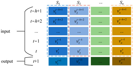
Figure 1.
Input and output of the prediction process.
2.2. Wind Farm Spatio-Temporal Relevance Analysis
The interaction and distribution of wind turbines cause the difference between the wind speed characteristics of multiple wind turbines and that of single wind turbines, which is known as the cluster effect [21]. Affected by the cluster effect, the wind speed of different position wind turbines has a certain temporal lag and spatial correlation. In the time domain, Recurrent Neural Network (RNN) and LSTM are commonly used to deal with wind speed temporal features [22]. Li et al. [23] proposed a hybrid model for wind speed interval prediction based on GRU and variational mode decomposition, which captures the temporal dependency in the wind speed sequence. However, considering its large computational cost, the training process will encounter problems such as gradient vanishing [24], which limits its ability to process the data of multi-wind turbines.
As more and more new energy sources are integrated into the power system, the time-series prediction of a single wind turbine is no longer sufficient to meet the accuracy requirement. Therefore, researchers try to extract the spatial feature information to reflect the complex relationship between multiple wind turbines.
We selected the wind speed data downloaded from the National Renewable Energy Laboratory (NREL, www.nrel.gov/grid/wind-toolkit.html (accessed on 30 July 2022)) of the United States for analysis. The data contains the wind speed data of five wind turbines on 1 January 2012, with a sampling interval of 5 min. The wind speed changes within one day are shown in Figure 2. In Section 1 and Section 2, it is obvious that although five wind speeds showed some delay characteristics, the overall change trend was consistent and reflected strong correlation between wind speeds of wind power generation units in the same space. This phenomenon motivates us to use the graph to represent the relationship of wind turbines in space.
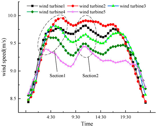
Figure 2.
Wind speed diagram of a wind farm.
2.3. Graph Theory
As is shown in Figure 3, a graph can be expressed as
where V represents the set of nodes, and E is the set of edges. Some related definitions are given as follows.
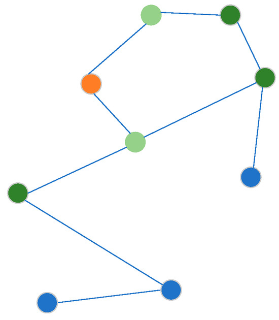
Figure 3.
The connected graph.
Definition 1.
(Adjacency Matrix). The adjacency matrix is a mathematical form of the graph, denoted as A∈with Aijif (vi,vj)E and Aijif (vi,vj)E.
Definition 2.
(Degree). The degree is the number of edges related to a vertex in the adjacency matrix, denoted by D. For directed graphs, the degree is divided into in-degree DI and out-degree DO, which represent the number of directed edges with the vertex as the end point or the start point, respectively.
Definition 3.
(Node Embedding). The node embedding is expressed as, where N is the number of nodes, d represents the dimension of node embedding, and dN. The node-embedding vector of the ith node is expressed as MiRd. Node embedding is a low-dimensional representation of a node of a graph that contains structural information [25,26].
3. Gated Attention Network Improved by Weighted Diffusion Graph Convolution
3.1. Definition of Multi-Wind Turbines Weighted Graph Structure
Topological graphs [27] are commonly used in power systems to describe the attributes and associations of nodes. Similarly, when processing multi-wind turbine data, each turbine can be regarded as a topological graph node. The node connections in the graph indicate the correlations between the speeds of wind turbines. Therefore, the definition of a multi-turbines graph is given by
where W = [wij]i, j =1, …, N, is the weight matrix that represents the correlations between nodes.
The specific steps for constructing the multi-wind turbine weighted diagram structure are given by:
- (i)
- Treat each wind turbine as a node, with nodes defaulting to interconnect, forming the basic topology structure for multiple turbines.
- (ii)
- On the basis of the original graph structure, we use wij to indicate the spatial correlation characteristics between wind turbines i and j. The larger the weight, the greater the mutual influence between turbines.
- (iii)
- Set a connection threshold α. If wij ≥ α, there is a strong correlation between node i and node j, and a connection is established. Otherwise, it is considered weakly correlated and wij = 0.
- (iv)
- Based on all the connected nodes, construct the weighted graph structure as shown in Figure 4.
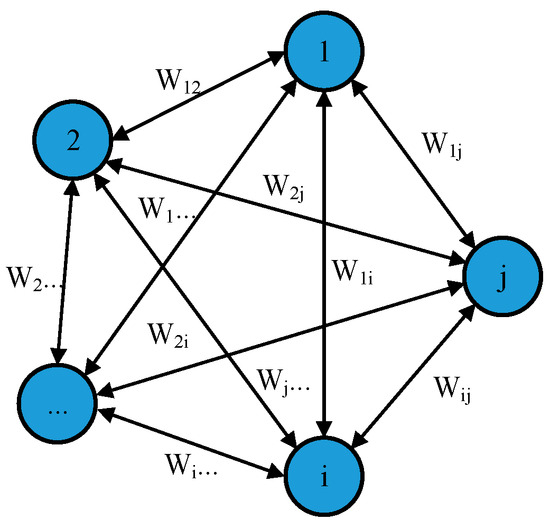 Figure 4. Multi-wind turbine weighted diagram structure.
3.2. Graph Weighting Calculation Based on MIC
In the wind farm graph structure, every node has different degrees and every connection has different weights [28]. The nodes in the center graph have higher values of degrees than the nodes on the edge. The degrees of the graph structure can describe the connections between nodes without considering the mutual influence of the wind speed between the turbines. It is necessary to redefine the connecting weight between nodes.
Mutual Information (MI) is an important concept in information theory, which represents the correlation of two random variables [29]. MIC is a statistic based on MI, which is used to measure the degree of association between two continuous variables. It can effectively distinguish between linear and non-linear relationships and has a consistent standard for different forms of relationships, with universality and fairness [30].
For any wind turbines, i and j, their wind speed sequence can be expressed as Si = and Sj = , where L is the length of sampling. The MIC calculation steps between turbine i and j are given as follows.
Step 1. MI calculation.
By dividing the value range of Si and Sj into several intervals, the mutual information between turbines i and j can be expressed as
where p(Si,Sj) is the joint probability density of turbines i and j under any grid partition scheme, and p(Si) and p(Sj) are the marginal probability density of turbines i and j, respectively.
Step 2. MI normalization.
The mutual information values under the same partition are min-max normalized as
Step 3. MIC expression.
The mesh division with the maximum mutual information value is recorded as Z = (s,t), where s and t, respectively, represent the number of intervals divided by the value range of Si and Sj. Then, MIC values of turbines i and j can be expressed as
where MIz(Si,Sj) represents the mutual information value under partition Z, and log2min{s,t} represents the normalized mutual information value. Then, the connection weight between nodes i and j can be expressed as
3.3. Gated Attention Network Improved by Weighted Diffusion Graph Convolution
The DGC network realizes the convolution operation on the non-Euclidean space through the forward and backward bidirectional diffusion process [31]. This diffusion feature is suitable for dealing with irregularly distributed multi-wind turbine data. As shown in Figure 5, the formula of weight DGC is given by
where and are adjustable training parameters, and are the out-degree diagonal matrix and in-degree diagonal matrix of the graph, respectively, and and are the forward diffusion matrix and backward diffusion matrix, respectively.
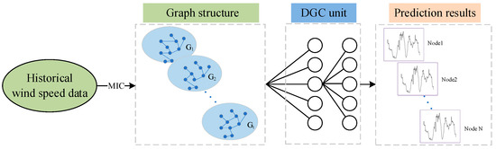
Figure 5.
Weighted diffusion graph convolution.
In order to ensure the complete extraction of spatio-temporal features of wind farms, we use DGC to calculate the weight matrices of the reset gate, update gate, and hidden state in GRU. Due to the fact that each turbine node contains its own historical information and the spatial information of the surrounding turbines at the same time, the network parameters and computational amount are increased. Therefore, the attention mechanism [32] is added to the output end of the GRU network, which focuses on the contribution of the hidden layer to the output, reduces the linear operations, and speeds up the network convergence. The improved gated attention network model is expressed as
and
where and represent the reset gate and the update gate, respectively, is the hidden state information at time t, and represent the state information of the previous and the next time steps, respectively, , , and are the bias terms, and tanh represent activation functions, is the attention function, and is the contribution of the ith hidden unit to the output at time t.
4. Model Prediction Framework
As shown in Figure 6, the operation process is given by the following process.
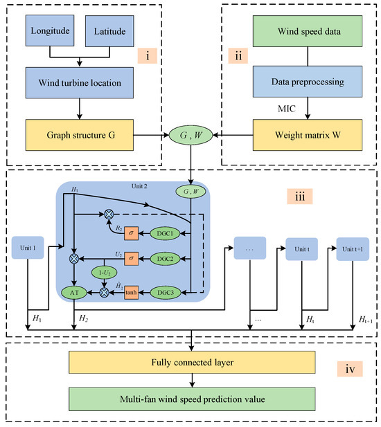
Figure 6.
Multi-wind turbine wind speed prediction model structure. The (i–iv) in the figure corresponds to the sequence numbers (i–iv) of the above operation process.
- (i)
- Construct the graph structure (G) of the wind farm based on the latitude and longitude of the wind turbines.
- (ii)
- Calculate the weight (W) by MIC between the turbine nodes in the graph.
- (iii)
- Input the graph G and the weight matrix W into the WDGCGAN model.
- (a)
- Spatial feature extraction. In each WDGCGAN unit, the DGC module calculates the diffusion convolution of graph G according to the weight matrix W. The obtained spatial feature matrix is output to each GRU gated module of the unit.
- (b)
- Temporal feature extraction. The spatial matrix is activated by the activation function and then spliced with the parameters of each gating and the state vector of the previous unit. The attention mechanism (AT) evaluates the contribution of the previous unit’s state vector and the current unit’s hidden state vector to the prediction result, allocates appropriate weights, and outputs the state vector of the current unit to the fully connected layer and the next unit.
- (iv)
- The fully connected layer is responsible for decoding the output of WDGCGAN units and obtains the multi-wind turbine wind speed prediction results containing spatio-temporal features.
5. Experimental Results and Analysis
5.1. Data Description
Experimental wind speed data was downloaded from the National Renewable Energy Laboratory (NREL, www.nrel.gov/grid/wind-toolkit.html (accessed on 30 July 2022)). The dataset contains ten wind turbines, whose distribution is shown in Figure 7.
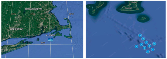
Figure 7.
Multi-wind turbine distribution.
The geographical coordinates and data statistics of each wind turbine are shown in Table 1. Based on the coordinates, the distance between adjacent wind turbines is about 4 km. The time ranges from 1 January 2012 to 31 December 2012 and the sampling interval is 5 min, which totals 102,120 data points. To ensure the temporal continuity of the data, we sequentially divided the raw dataset into training and testing sets with a ratio of 8:2.

Table 1.
The statistics of the wind speed data.
5.2. Models and Experimental Setup
In this paper, we set up six representative multi-turbine prediction models as benchmark models and comprehensively validated the prediction performance of the proposed model.
CNN [14] and LSTM [4] are classic models in the prediction field, commonly used to handle time-series prediction tasks. CNN-LSTM [15] is a linear combination model based on CNN and LSTM, used to process the temporal and spatial features in the sequence. WDGC_GAN is a linear combination of a graph convolutional network and gated attention network after weighting. DGCGAN and WDGCGRU are derived models based on the model in this paper. DGCGAN refers to not performing graph structure weighting on the basis of the model in this paper, while WDGCGRU refers to removing the added attention mechanism on the basis of the model in this paper. The model parameter settings are given in Table 2.
Table 2.
Model parameter settings.
In this experiment, all the models were built under the same deep learning platform, with the RedHat 64-bit operating system environment, Pytorch1.8-based model framework, RTX-3060 hardware GPU model, 16G memory, AMD Ryzen 7-5800H CPU @ 3.20GHz, and Python3.9.
In order to quantitatively and comprehensively evaluate the multi-wind turbines prediction model, we chose the coefficient of determination (R2), root mean square error (RMSE) and mean absolute percentage error (MAPE) as the evaluation criterions
where n represents the number of samples in the dataset, denotes the actual wind speed value for the i-th sample, signifies the model’s predicted value for the i-th sample, and denotes the average value of the wind speed.
5.3. Multi-Wind Turbine Prediction Results Analysis
We set the threshold of node connection = 0.8 and input the weighted graph structure of the multi-wind turbine into the trained WDGCGAN model for spatio-temporal feature extraction. The prediction results are output at the end. The prediction error is given in Table 3 and the MIC values between multiple turbines are shown in Figure 8a.
Table 3.
The forecast error of ten wind turbines.
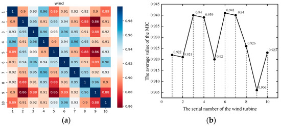
Figure 8.
The correlation description of wind turbines. (a) The MIC thermodynamic diagram between wind turbines. (b) The average wind speed MIC of the wind turbines.
After the prediction task was completed, we compared the prediction error level and the MIC heat map of the ten wind turbines. As shown in Table 3, the R2, RMSE, and MAPE indicators of the 3rd, 4th, 6th, and 7th wind turbines perform excellently. At the same time, we calculated the average MIC value of each wind turbine with other wind turbines, as shown in Figure 8b. The average MIC of the ith wind turbine is calculated by
We found that the average MIC values of the 3rd, 4th, 6th, and 7th wind turbines were better than other wind turbines. This indicates that the 3rd, 4th, 6th, and 7th wind turbines can better aggregate the historical information of the surrounding wind turbines, which helps to improve the model prediction accuracy. At the same time, this also verifies the conclusion that the 3rd, 4th, 6th, and 7th wind turbines have excellent prediction errors.
To improve the forecasting indicators, we studied the number of training iterations for the model parameters. Keeping the other parameters constant, we tried different numbers of model training iterations and recorded the corresponding training times. The relationship between the number of training iterations and the total average prediction error is shown in Figure 9.
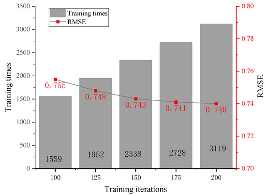
Figure 9.
The average prediction error at different iterations.
As we can see in the figure, as the number of training iterations increases, the prediction error tends to decrease. Additionally, since the number of iterations is closely linked to training time, an increase in iterations also leads to an increase in training time, and the rate of increase in training time is greater than the decrease in prediction error. Considering the greater impact of the number of iterations on training time, we have chosen a training count of 100.
5.4. Spatio-Temporal Model Prediction Performance Comparison
To analyze the prediction performance of the model in different seasons, this section divides the wind speed dataset into spring (January to March), summer (April to June), autumn (July to September) and winter (October to December). The wind speed statistics for the four seasons are given in Table 4.
Table 4.
Seasonal wind speed statistics.
The average wind speed in spring was 7.06 m/s, the standard deviation was 3.29 m/s, and the maximum wind speed was 22.35 m/s. The average wind speed in winter was 9.66 m/s, the standard deviation was 4.83 m/s, and the maximum wind speed was 37.41 m/s. We found that the wind speed changes were relatively smooth in spring, while the wind speed fluctuations were intense in winter, when the wind speed extremes were the highest.
We experimented with the proposed model and the traditional spatio-temporal prediction models LSTM, CNN, and CNN-LSTM in different seasons to evaluate the model prediction performance. The model parameters are shown in Table 2. The RMSE of the prediction results are given by Figure 10.
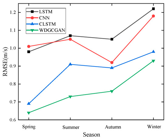
Figure 10.
RMSE of prediction error of comparison model.
In Figure 10, we found that the prediction errors RMSE of each model gradually increased from spring to winter. Combined with Table 4, it can be known that this is because the standard deviation of wind speed data gradually increased from spring to winter, the degree of wind speed fluctuation gradually intensified, and thus affected the prediction accuracy of the model. However, the proposed model is still superior to the comparison model in each season.
The prediction results of the comparison model are given in Table 5. We found that the proposed model outperforms the comparison model in all four seasons.
Table 5.
Comparison of spatio-temporal models.
In the 30 min prediction task, the average RMSE of our model was 26.4% and 29.1% lower than that of CNN and LSTM, respectively. CNN and LSTM have large prediction errors in each season, because they are single models that can only extract limited spatial or temporal features. The average RMSE of our model was 11.8% lower than CLSTM. Generally, the multi-wind turbine distribution is irregular. The CLSTM needed to fill in the missing parts with zeros when processing the space features, which increased irrelevant information and affected the final prediction result. Otherwise, the proposed model constructs a graph structure that can describe the arbitrary shape of the wind farm.
In the 1h prediction task, the prediction scale increased, making the time dependence in the time series harder to capture. The prediction errors of each model increased compared with the 30 min prediction. However, the proposed model still outperformed the comparison models, with the average RMSE being 28%, 33.1%, and 16.5% lower than that of LSTM, CNN, and CLSTM, respectively.
5.5. Ablation Experiment Analysis
In this section, we split the historical wind speed data of 2012 at a ratio of 8:2 and compared the prediction performance of the WDGC_GAN, DGCGAN, WDGCGRU, and WDGCGAN models. The parameter settings of these models are given in Table 2.
We evaluated the models on three aspects: the prediction accuracy of the weighted graph construction method, the effectiveness of improving GRU by DGC embedding operation, and the effectiveness of the attention mechanism on model performance. The prediction results of ablation model are expressed in Figure 11.
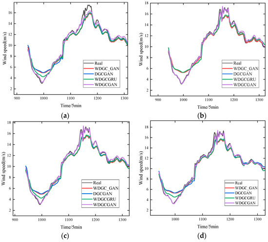
Figure 11.
Prediction results of the ablation model. (a) The prediction results of the 1st wind turbine. (b) The prediction results of the 4th wind turbine. (c) The prediction results of the 7th wind turbine. (d) The prediction results of the 10th wind turbine.
Due to space limitations, we only show the prediction results of the 1st, 4th, 7th, and 10th wind turbines. The WDG_GAN model’s prediction results differ greatly from the actual values and fail to capture the wind speed change trend. The DGCGAN and WDGCGRU models can predict the future wind speed signal trend correctly, but they have errors at the peaks and valleys due to the data’s violent fluctuation. The WDGCGAN model can learn the wind speed trend better and obtain more accurate multi-wind turbine wind speed prediction results.
We take the 10th wind turbine as an example for a detailed analysis. The prediction error of the 10th wind turbine is shown in Table 6.
Table 6.
Prediction error of the 10th wind turbine.
In contrast to DGCGAN, WDGCGAN reduces the prediction errors of RMSE and MAPE by 0.22 m/s and 3.72%, respectively, with almost no change in the training time. It shows that the weighted graph structure can better characterize the correlation of the multi-wind turbine.
Compared with WDG_GAN, WDGCGAN increases the parameter amount and the training time by 6.4s due to the DGC operations. But, it reduces the errors of RMSE and MAPE by 0.26m/s and 3.84%, respectively. With a small increase in the training time, it shows that the weighted DGC operation can effectively extract the spatio-temporal features of the multi-wind turbine data and improve the prediction model performance.
Unlike WDGCGRU, WDGCGAN reduces the training time by 38.4 s and decreases the RMSE and MAPE by 0.06m/s and 0.16%, respectively. It shows that the attention mechanism in our model can speed up the model training and slightly improve the prediction accuracy.
By comparison, the WDGCGAN model has excellent performance on indicators such as R2, RMSE, and MAPE, indicating its contribution to the accuracy and stability of wind speed prediction. In contrast, the combined model WDGC-GAN has the worst prediction performance, with higher RMSE and MAE values and a lower R2 value, reflecting relatively low prediction accuracy.
6. Conclusions
The core of this paper is to study the structure and modeling method of the spatial relationships between wind speeds, to extract the wind speed characteristics of irregular wind farms more effectively, and to achieve multi-turbine wind speed prediction. We proposed a multi-wind turbine wind speed prediction method based on the weighted graph structure and WDGCGAN. The following conclusions are drawn from the case:
- (i)
- There is a spatial correlation between the wind speeds of the wind turbines in the same wind farm. We can use the maximum mutual information of the wind speed between the wind turbines to express and model the spatial relationship of multiple wind turbines and the inclusion of wind speed features with strong correlation also helps to improve the prediction performance of the model.
- (ii)
- The experiments show that the model with the maximum mutual information spatial correlation module and the attention mechanism can reduce the prediction error of the model and make the prediction curve of each wind turbine closer to the true value of the wind speed. In the 1h prediction task, the average RMSE was 28%, 33.1%, and 16.5% lower than that of LSTM, CNN, and CLSTM, respectively.
- (iii)
- Based on the efficient modeling of the spatial relationship of multiple wind turbines, our next work will consider using correlation analysis, random forest, and the conclusion of the maximum mutual information in Section 5.3 of this manuscript to select the wind parameter feature variables that are strongly correlated with the wind speed prediction, such as wind speed duration, wind direction, etc., and jointly construct a large-scale variable weighting graph to express their complex correlation relationship.
- (iv)
- In future work, we plan to model for different types of wind farms and conduct multi-turbine wind speed forecasting for more nodes. We will try to use optimization algorithms to find the optimal parameters for the model. Additionally, based on the existing wind speed correlation modeling, we also hope to extend the model to the wind power domain, achieving synchronous forecasting of multi-turbine wind power.
Author Contributions
Conceptualization, Y.Q. and H.C.; methodology, Y.Q. and B.F.; software, Y.Q.; validation, Y.Q. and B.F.; formal analysis, H.C.; investigation, Y.Q.; resources, H.C.; data curation, Y.Q.; writing—original draft preparation, Y.Q.; writing—review and editing, Y.Q. and B.F.; visualization, H.C.; supervision, B.F.; funding acquisition, B.F. All authors have read and agreed to the published version of the manuscript.
Funding
This research was supported by the Key Research and Development Program of Hubei Province, China (grant number 2021BAA193).
Data Availability Statement
The original contributions presented in the study are included in the article, further inquiries can be directed to the first author.
Conflicts of Interest
The authors declare no conflicts of interest.
References
- Exizidis, L.; Kazempour, S.J.; Pinson, P. Sharing Wind Power Forecasts in Electricity Markets: A Numerical Analysis. Appl. Energy 2016, 176, 65–73. [Google Scholar] [CrossRef]
- Ma, Z.; Chen, W.H.; Wang, J. Application of Hybrid Model Based on Double Decomposition, Error Correction and Deep Learning in Short-Term Wind Speed Prediction. Energy Convers. Manag. 2020, 205, 112345. [Google Scholar] [CrossRef]
- Gao, Z.; Li, Z.; Xu, L. Dynamic Adaptive Spatio-Temporal Graph Neural Network for Multi-Dode Offshore Wind Speed Forecasting. Appl. Soft Comput. 2023, 141, 110294. [Google Scholar] [CrossRef]
- Huang, Y.; Zhang, B.; Pang, H. Spatio-Temporal Wind Speed Prediction Based on Clayton Copula Function with Deep Learning Fusion. Renew. Energy 2022, 192, 526–536. [Google Scholar] [CrossRef]
- Yang, M.; Chen, Y.L. Real-Time Prediction for Wind Power Based on EMD and Set Pair Analysis. Trans. China Electrotech. Soc. 2016, 31, 86–93. [Google Scholar]
- Xu, X.; Xie, L.R.; Liang, W.X. Bi-Level Optimization Model Considering Time Series Characteristic of Wind Power Forecast Error and Wind Power Reliability. Trans. China Electrotech. Soc. 2023, 38, 1620–1632+1661. [Google Scholar]
- Candy, B.; ES, J.; Keogh, S.J. A Comparison of the Impact of QuikScat and WindSat Wind Vector Products on Met Office Analyses and Forecasts. IEEE Trans. Geosci. Remote Sens. 2009, 47, 1632–1640. [Google Scholar] [CrossRef]
- Sun, W.; Gao, Q. Short-Term Wind Speed Prediction Based on Variational Mode Decomposition and Linear–Nonlinear Combination Optimization Model. Energies 2019, 12, 2322. [Google Scholar] [CrossRef]
- Liu, X.L.; Lin, Z.; Fang, Z.M. Short-term offshore wind speed forecast by seasonal ARIMA-A comparison against GRU and LSTM. Energy 2021, 227, 120492. [Google Scholar] [CrossRef]
- Zhang, H.; Chen, L.; Qu, Y. Support Vector Regression Based on Grid-Search method for short-term wind power forecasting. J. Appl. Math. 2014, 2014, 835791. [Google Scholar] [CrossRef]
- Ma ngalova, E.; Agafonov, E. Wind Power Forecasting Using the K-Nearest Neighbors Algorithm. Int. J. Forecast. 2014, 30, 402–406. [Google Scholar] [CrossRef]
- Liao, W.; Wang, S.; Bak-Jensen, B. Ultra-Short-Term Interval Prediction of Wind Power Based on Graph Neural Network and Improved Bootstrap Technique. J. Mod. Power Syst. Clean Energy 2023, 11, 1100–1114. [Google Scholar] [CrossRef]
- He, Y.; Chai, S.; Zhao, J. A Robust Spatio-Temporal Prediction Approach for Wind Power Generation Based on Spectral Temporal Graph Neural Network. IET Renew. Power Gener. 2022, 16, 2556–2565. [Google Scholar] [CrossRef]
- Zhu, Q.M.; Chen, J.F.; Zhu, L. Wind Speed Prediction with Spatio–Temporal Correlation: A Deep Learning Approach. Energies 2018, 11, 705. [Google Scholar] [CrossRef]
- Zhen, H.; Niu, D.; Yu, M. A Hybrid Deep Learning Model and Comparison for Wind Power Forecasting Considering Temporal-Spatial Feature Extraction. Sustainability 2020, 12, 9490. [Google Scholar] [CrossRef]
- Asif, N.A.; Sarker, Y.; Chakrabortty, R.K. Graph Neural Network: A Comprehensive Review on Non-Euclidean Space. IEEE Access 2021, 9, 60588–60606. [Google Scholar] [CrossRef]
- Yu, M.; Zhang, Z.; Li, X. Superposition Graph Neural Network for Offshore Wind Power Prediction. Future Gener. Comput. Syst. 2020, 113, 145–157. [Google Scholar] [CrossRef]
- Khodayar, M.; Wang, J. Spatio-Temporal Graph Deep Neural Network for Short-Term Wind Speed Forecasting. IEEE Trans. Sustain. Energy 2018, 10, 670–681. [Google Scholar] [CrossRef]
- Li, Y.G.; Yu, R.; Shahabi, C. Diffusion Convolutional Recurrent Neural Network: Data-Driven Traffic Forecasting. arXiv 2017, arXiv:1707.01926. [Google Scholar]
- Li, Y.; Shen, X.; Zhou, C. Dynamic Multi-Turbines Spatio-Temporal Correlation Model Enabled Digital Twin Technology for Real-Time Wind Speed Prediction. Renew. Energy 2023, 203, 841–853. [Google Scholar] [CrossRef]
- Cao, J.; Qin, Z.; Gao, X. Study of Aerodynamic Performance and Wake Effects for Offshore Wind Farm Cluster. Ocean Eng. 2023, 280, 114639. [Google Scholar] [CrossRef]
- Qian, J.; Zhu, M.; Zhao, Y. Short-Term Wind Speed Prediction with A Two-Layer Attention-Based LSTM. Comput. Syst. Sci. Eng. 2021, 39, 197–209. [Google Scholar] [CrossRef]
- Li, C.; Tang, G.; Xue, X. Short-Term Wind Speed Interval Prediction Based on Ensemble GRU Model. IEEE Trans. Sustain. Energy 2019, 11, 1370–1380. [Google Scholar] [CrossRef]
- Turkoglu, M.O.; D’Aronco, S.; Wegner, J.D. Gating Revisited: Deep Multi-Layer RNNs That Can Be Trained. IEEE Trans. Pattern Anal. Mach. Intell. 2021, 44, 4081–4092. [Google Scholar] [CrossRef]
- Liu, J.; Yang, X.; Zhang, D. Adaptive Graph-Learning Convolutional Network for Multi-Node Offshore Wind Speed Forecasting. J. Mar. Sci. Eng. 2023, 11, 879. [Google Scholar] [CrossRef]
- Bai, L.; Yao, L.; Li, C. Adaptive Graph Convolutional Recurrent Network for Traffic Forecasting. Adv. Neural Inf. Process. Syst. 2020, 33, 17804–17815. [Google Scholar]
- Gao, H.; Yu, X.; Sui, Y. Topological Graph Convolutional Network Based on Complex Network Characteristics. IEEE Access 2022, 10, 64465–64472. [Google Scholar] [CrossRef]
- Lu, J.; Mutee-ur-Rehman, H.; Nazeer, S. The Edge-Weighted Graph Entropy Using Redefined Zagreb Indices. Math. Probl. Eng. 2022, 2022, 5958913. [Google Scholar] [CrossRef]
- Jency, W.G.; Judith, J.E. Homogenized Point Mutual Information and Deep Quantum Reinforced Wind Power Prediction. Int. Trans. Electr. Energy Syst. 2022, 2022, 3686786. [Google Scholar] [CrossRef]
- Wei, J.; Wu, X.; Yang, T. Ultra-Short-Term Forecasting of Wind Power Based on Multi-Task Learning and LSTM. Int. J. Electr. Power Energy Syst. 2023, 149, 109073. [Google Scholar] [CrossRef]
- Liang, F.; Qian, C.; Yu, W. Survey of Graph Neural Networks and Applications. Wirel. Commun. Mob. Comput. 2022, 2022, 9261537. [Google Scholar] [CrossRef]
- Brauwers, G.; Frasincar, F. A General Survey on Attention Mechanisms in Deep Learning. IEEE Trans. Knowl. Data Eng. 2021, 35, 3279–3298. [Google Scholar] [CrossRef]
Disclaimer/Publisher’s Note: The statements, opinions and data contained in all publications are solely those of the individual author(s) and contributor(s) and not of MDPI and/or the editor(s). MDPI and/or the editor(s) disclaim responsibility for any injury to people or property resulting from any ideas, methods, instructions or products referred to in the content. |
© 2024 by the authors. Licensee MDPI, Basel, Switzerland. This article is an open access article distributed under the terms and conditions of the Creative Commons Attribution (CC BY) license (https://creativecommons.org/licenses/by/4.0/).