FEM Simulation of Fault Reactivation Induced with Hydraulic Fracturing in the Shangluo Region of Sichuan Province

Abstract

Hydraulic fracturing operations possess the capacity to induce the reactivation of faults, increasing the risk of fault slip and seismic activity. In this study, a coupled poroelastic model is established to characterize the distribution and movement of fluids within rock formations in the Shangluo region of Sichuan province, China. The effect of hydraulic fracturing projects on the variations of pore pressure and Coulomb effective stress within a high-permeability fault is analyzed. The potential fault-slip mechanism is investigated. The results show that the fault plays different roles for fluid movement, including the barrier, fluid transport channel, and diversion channel, which is related to injection–production schemes. In addition, fluid injection leads to a high probability of fault reactivation. We find that increasing the injection time and fluid injection rate can result in larger slip distances. The injection production scenarios influence the fault-slip mechanism, resulting in a normal fault or reverse fault. However, the arrangement of production wells around the injection can effectively reduce the risk of fault reactivation.

1. Introduction

Shale gas, as an unconventional energy source, has gained significant attention. Recently, the occurrence of fault reactivation induced by fluid injection during the stimulation process has been widely concerning for researchers [1,2,3]. Previous studies highlighted the influence of both geologic and engineering factors, such as pre-existing fractures and hydraulic fracturing schemes, on fault slip and earthquakes [4,5,6]. Fault activity is deemed to be associated with fracturing operations [7]. Slow and steady slip occurring on major faults in the vicinity of some shale gas wells during fracturing process is observed [8,9]. Observations show that fault slip leads to casing deformation and the changes in shear stress during fault activity are associated with seismic events [10,11,12]. Currently, the Shangluo region in Sichuan has become a mature shale gas development area, where five earthquakes with magnitudes greater than 4.0 (M_W > 4.0) occurred during hydraulic fracturing operations [13,14]. The largest event (M_W 4.7) took place on 28 January 2017. Significant surface deformation due to fault reactivation was observed [15]. Understanding the mechanisms and control measures of fault reactivation induced by hydraulic fracturing is crucial for seismic monitoring and mitigation during shale gas exploitation.

Fault-slip events are influenced by multiple factors, such as stress state [16,17], fluid properties [18,19,20], temperature [21,22], and the combined impact of various factors [23,24]. Cyclical injection and production cause stress perturbations that lead to seismic activities around fault zones [22,25]. The maximum magnitude of seismic activities occurs during the injection phase of the fracturing fluid. Even small stress changes during the production flowback phase reactivate the faults and generate a large number of seismicity events [26,27]. Based on laboratory and field experiments on the permeability and frictional properties of faults [28], it is possible that stress changes during the fracturing process could induce fault reactivation, leading to long-distance fault slips [29].

Numerical models for describing fault slip induced by hydraulic fracturing remain a challenge. There are two categories of numerical methods for the simulation of rock fracturing processes: discontinuous methods and continuous methods. The discontinuous methods most commonly used are based on linear elastic fracture mechanics (LEFM), which include cohesive zone models (CZM) and discrete fracture network models (DFN).

DFN is a commonly used discontinuity method. Initially, a semi-analytical numerical model for the calculation of induced stresses along hydraulic fractures was developed [30]. The influence of fracture initiation location, fluid pressure, fracture dip, and friction factor on fracture slip was discussed. It was found that the region of high-pressure fluid flow has a higher risk of fault reactivation, while the fluid flows at the bottom of the fault could reduce the fault-slip distance. In the DFN model, the effect of fault reactivation is realized by stress perturbation. The DFN model can reflect the characteristics of fluid–solid coupling in the shear process, where crack opening caused by fluid injection can lead to formation slip [31]. After improving the discrete fracture model, a test was conducted to demonstrate that the method has lower computational cost and more desirable convergence performance than the standard DFM [32]. Subsequently, to further improve the DFN model [33], both static and dynamic induced effects were considered, which could simulate the seismic response in a fractured rock mass. The DFN method approach can represent the injection-induced stress perturbations and pore pressure changes well, but there are still many problems in modelling large deformations and long-distance sliding of faults.

The method of combining continuous and discontinuous method is more widely used for considering excessive displacement. Many researchers have used FLAC3D to simulate hydraulic fracturing under a variety of conditions, including direct injection [5,21], staged injection [34], and isothermal water injection [35]. The possibility of fluid injection induced seismicity was discussed. The stress change during fracturing was explained by considering pore pressure diffusion and poroelastic effects. By monitoring the hydraulic behavior in the rock matrix and along the fault, it was found that the fault is more likely to be reactivated when the shear stress is dominant. In addition, the magnitude of removing grouting induced seismic activity is also influenced by the unequal distribution of fault-slip time. Rocks with lower modulus show greater slip distance and seismic activity during shear failure. Some researchers focused on the issue of fracture propagation during fluid injection and developed a fully coupled continuous and discontinuous method [36,37] to simulate fluid pressure and fracture propagation mode in porous media. The results show that the conversion between fracture propagation modes depends on the injection flow rate.

While stress perturbations within faults during hydraulic fracturing operations have been widely investigated, the mechanisms underlying induced fault slip have not been thoroughly studied. Moreover, predicting the trend of slip motion and understanding the effects of injection remain crucial unresolved issues. In this study, a fully coupled fluid–solid geomechanical model is proposed to simulate the response of a fault, and then the seismic theory is applied to estimate the magnitude of the seismicity. Three important factors affecting the fault slip behavior are discussed: injection time, injection rate, and production scenarios. This research aims to provide a numerical method for assessing induced seismic events and fault slip distance, and to clarify the mechanisms underlying hydraulic fracturing on fault slip events.

2. Methodology

2.1. Coupled Poroelastic Model

The coupled poroelastic model describes how a saturated porous elastic medium responds to changes in stress and pore pressure. According to this model, changes in pore pressure could affect the pore elastic stress of the medium and, conversely, changes in stress could affect the pore pressure [38].

The formulation of consolidation in poroelastic media is given as follows. The displacement vector $u$ captures the deformation of the solid skeleton, and then the strain tensor $\epsilon$ at a point inside the deformable medium is expressed according to the following assumption [39]:

$$\epsilon =\frac{1}{2}\left({\left(𝛻u\right)}^T+\left(𝛻u\right)\right)$$

(1)

The equilibrium condition of stress field in the deformable medium is provided based on the poroelastic theory:

$$𝛻·\sigma +f=0$$

(2)

where $f$ is the body force. The total stress tensor reads $\sigma ={\sigma }_{ex}+\mathbb{C}:(\epsilon -{\epsilon }_{inel})$, where $\mathbb{C}$ is the 4th order elasticity tensor, and “$:$” refers to the double-dot tensor product (or double contraction). The elastic strain ${\epsilon }_{el}$ is the difference between the total strain $\epsilon$ and all inelastic strains ${\epsilon }_{inel}$. There may also be an extra stress contribution ${\sigma }_{ex}$ with contributions from initial stresses and viscoelastic stresses. Therefore, Equation (2) is rewritten as

$$𝛻·({\sigma }_{ex}+\mathbb{C}:(\epsilon -{\epsilon }_{inel}\left)\right)+f=0$$

(3)

The constitutive equations for a saturated fluid-filled porous elastic medium can be expressed as [38,40]

$$G{𝛻}^{2}u+\frac{G}{1-2v}𝛻{\epsilon }_{vol}-{\alpha }_B𝛻p=0$$

(4)

where $G$ is the shear modulus, $u$ is the velocity field, $v$ is Poisson’s ratio, ${\epsilon }_{vol}$ is the volumetric strain, ${\alpha }_B$ is the Biot coefficient, and $𝛻p$ is the applied pressure gradient.

The pore fluid mass conservation equation can be expressed with [41]

$$\frac{\partial }{\partial \mathrm{t}}\left({\epsilon }_p{\rho }_f\right)+𝛻·\left(\rho u_p\right)=Q_m$$

(5)

where ${\rho }_f$ is fluid density, ${\epsilon }_p$ is the medium’s porosity, and $Q_m$ is the fluid mass source. To account for the coupling between fluid and solid fields, the storage coefficient S is defined as the weighted compressibility of both [42], which can be calculated from Equation (3):

$$S={\epsilon }_p{\chi }_f+\frac{\partial {\epsilon }_p}{\partial p}$$

(6)

$$\frac{\partial }{\partial \mathrm{t}}\left({\epsilon }_p\rho \right)=\rho S\frac{\partial p}{\partial t}$$

(7)

Fluid flow in a porous elastic medium is described with Darcy’s law. The velocity of the flow in the flow field is calculated with

$$u_p=-\frac{k}{\mu }(𝛻p+{\rho }_{f}g𝛻D)$$

(8)

where $u_p$ is the Darcy’s velocity, $k$ is the permeability of the medium, $\mu$ is the fluid viscosity, $𝛻D$ is the difference in elevation.

Therefore, the mass conservation equation is eventually rewritten as

$${\rho }_{f}S\frac{\partial p}{\partial t}+𝛻\cdot {\rho }_f\left[-\frac{k}{\mu }\left(𝛻p+{\rho }_{f}g𝛻D\right)\right]=Q_m-{\rho }_f{\alpha }_B\frac{\partial }{\partial t}{\epsilon }_{vol}$$

(9)

Assuming that the fluid flow process is a saturated flow process, the flow equations specified by Darcy’s law are satisfied. To ensure accuracy, substantial grid refinement is required in the vicinity of interfaces with rapidly changing permeability, such as between faults and cap rocks. Failure to meet the accuracy requirements of mesh discretization may result in anomalous pore pressure oscillations and reduced convergence rates.

2.2. Strain–Permeability Model

This study utilizes a function based on porosity and volumetric strain to express the permeability variation in the model. In addition, the approach proposed by Cappa and Rutqvist [43] is used to represent the permeability of fracture zones, which links fracture aperture and fracture spacing:

$$k=\frac{b^3}{12s}$$

(10)

where k is the permeability of fault, b is the pore diameter, and s is the fracture width. The permeability is affected by both tensile and shear fracturing, which adds to the initial fault permeability. Rutqvist et al. (2013) [44] used the permeability variation model that took into account the plastic strain along a fault, which is positively correlated with the fault plane:

$$k=k_0+k_f=k_0+A{({\epsilon }_n-{\epsilon }_n^t)}^3$$

(11)

where $k_0$ is the initial permeability of fault, $A$ is the constant, and ${\epsilon }_n^t$ is the threshold strain, which represents the strain at the moment when the fault first starts to slip. This study uses ${\epsilon }_n^t$ = 1 × 10⁻⁴ and A = 1 × 10⁻⁵, indicating a potential increase in permeability by three orders of magnitude. This permeability variation is significant compared to the initial fault permeability. As the fractures propagate, pressure diffuses rapidly within the rock mass.

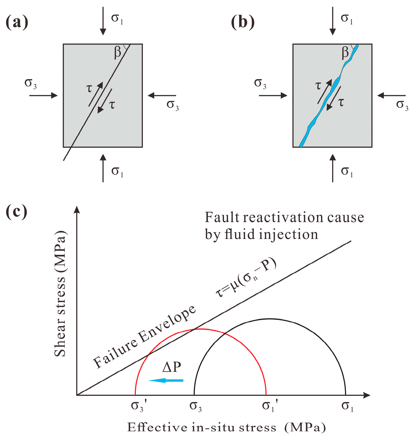
2.3. Coulomb Failure Stress Changes

The Coulomb failure envelope can be estimated based on the rock strength properties, such as the friction angle, cohesion, and tensile strength. Before injection, faults are commonly in either a critical or stable stress condition (Figure 1a). However, the significant change in pore pressure caused by the injection of water can induce the reactivation of the fault (Figure 1b). When the pressure of fluid injection reaches a certain level, it can cause slip (shear failure) by exceeding the failure envelope [45]. Figure 1c illustrates the contraction of the Mohr circle, where the change in the vertical principal stress is determined by the variations in applied load pressure and the Biot coefficient, while the change in the horizontal principal stress is related to the rock’s Poisson’s ratio [21,46,47]. In this situation, the hydraulic fracture does not directly contact the fault, but the rock is elastically deformed during injection. This change in the local stress field near the fault can activate the fault, as shown in Figure 1c, where the Mohr circle approaches the Coulomb failure envelope.

By utilizing the updated stress state, the evolution of Coulomb failure stress (∆CFS) during the injection and production processes can be obtained [48] with

$$\mathsf{\Delta }CFS=\mathsf{\Delta }\tau -\mathsf{\Delta }{\sigma }_n^{\prime }=\left(\mathsf{\Delta }\tau -{\mu }_s\mathsf{\Delta }{\sigma }_n\right)+{\mu }_s\mathsf{\Delta }{P}_p$$

(12)

$${\sigma }_n=\frac{1}{2}\left({\sigma }_1+{\sigma }_3\right)-\frac{1}{2}\left({\sigma }_1-{\sigma }_3\right)\mathit{cos}\left(2\beta \right)$$

(13)

$${\sigma }_n^{\prime }={\sigma }_n-P_p$$

(14)

$$\tau =\frac{1}{2}\left({\sigma }_1-{\sigma }_3\right)\mathit{sin}\left(2\beta \right)$$

(15)

where $\tau$ is the shear stress, ${\sigma }_n$ is the total normal stress, ${\mu }_s$ is the coefficient of static friction, and $P_p$ is the pore pressure. The Coulomb failure criterion relates the frictional strength of the fault to two factors: (1) the Terzaghi effective stress (${\sigma }_n-P_p$) and (2) the coefficient of static friction, ${\mu }_s$, which is commonly assumed to range between 0.6 and 0.8. It is assumed that the frictional properties along the fault plane are homogeneous and the representative value of the static friction coefficient, ${\mu }_s$, is taken as 0.6.

3. Numerical Model

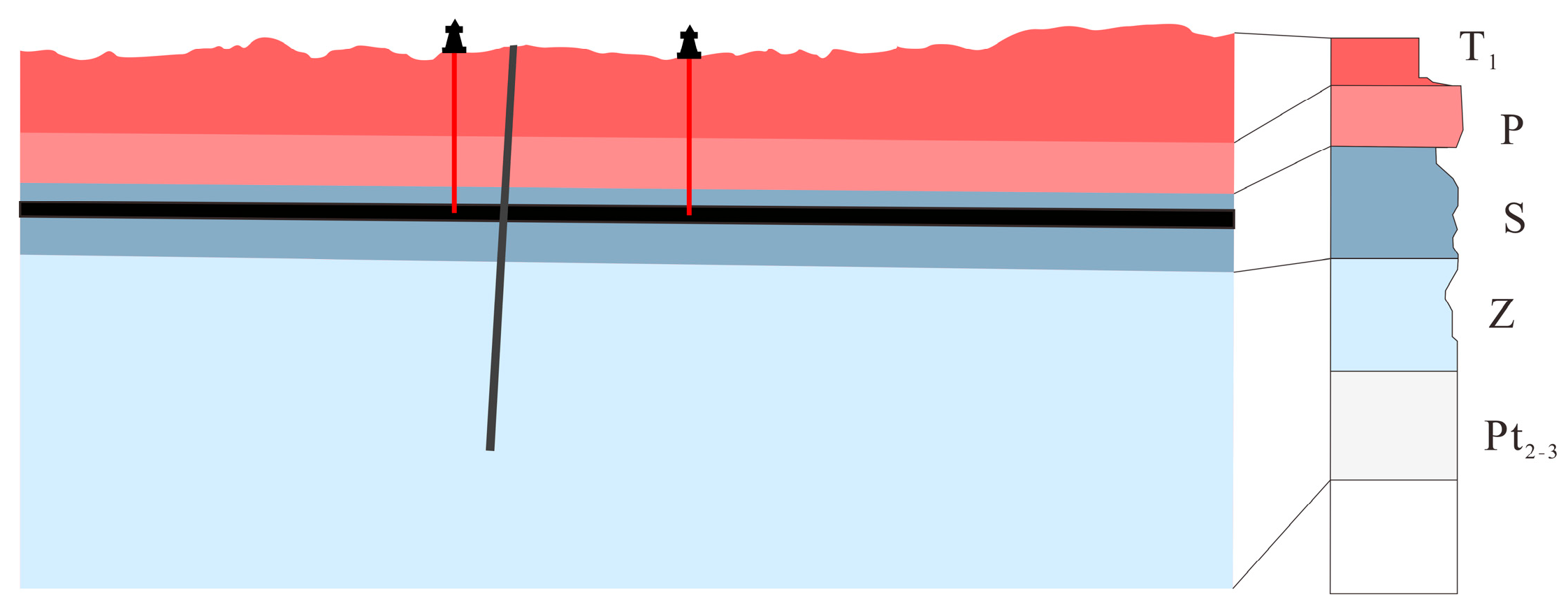
3.1. Geologic Model and Boundary Conditions

The study area is located in the Shangluo region of Sichuan province, China. A finite element model was established to simulate the injection process with COMSOL Multiphysics 6.0. The model has a length of 24,000 m and a height of 12,000 m, as shown in Figure 2. Three different distances between the injection well and the fault were set, as shown in Figure 3a: (a) d = 150 m, (b) d = 450 m, and (c) d = 750 m. To investigate the influence of injection/production schemes on fault slip, three different configurations were set in the simulations: (1) case 1 with two injection wells; (2) case 2 with one injection well located on the hanging wall of the fault and one production well located on the footwall of the fault; and (3) case 3 with one injection well located on the footwall of the fault and one production well located on the hanging wall of the fault (Figure 3b). Note that the spacing D between two wells in each case is fixed at 1500 m.

The sedimentary sequence of the study area consists of a dense, low-permeability limestone caprock, a shale reservoir and a fault. The material properties are presented in

Table 1. Material properties used in the models.

Category	Limestone	Shale	Fault
$\mathrm{Young}\text{’}\mathrm{s}\mathrm{Modulus}E/\mathrm{G}\mathrm{P}\mathrm{a}$	47.1	26.2	5
$\mathrm{Poisson}\mathrm{ratio}\nu$	0.12	0.2	0.25
$\mathrm{Porosity}{\epsilon }_p$	0.015	0.025	0.04
$\mathrm{Permeability}{\mathrm{k}/\mathrm{m}}^2$	1.00 × 10−19	3.00 × 10−17	2.35 × 10−14
$\mathrm{Cohesive}\mathrm{force}c/\mathrm{M}\mathrm{P}\mathrm{a}$	30.4	16.2	0
$\mathrm{Internal}\mathrm{friction}\mathrm{angle}\phi /°$	46.2	36.2	31
$\mathrm{Rock}\mathrm{density}{\rho }_s/(\mathrm{k}\mathrm{g}/{\mathrm{m}}^3)$	2700	2700	2700
$\mathrm{Fluid}\mathrm{density}{\rho }_f/(\mathrm{k}\mathrm{g}/{\mathrm{m}}^3)$	1050	1050	1050
$\mathrm{Biot}\mathrm{coefficient}{\alpha }_B$	0.8	0.8	0.8

[49]. The hydraulic fracturing target is the Longmaxi shale formation, which is buried at a depth of approximately 2.7 to 3 km. The reservoir has a thickness of approximately 200 m and is restricted by adjacent layers with very low porosity and permeability. The fault, which has a dip angle of 80°, is 40 m thick. It is commonly characterized as comprising a fault core and the surrounding damage zone [50,51,52].

3.2. Boundary Condition and Parameter Setting

The solid mechanics equations are subject to roller support boundary conditions on both the left and right sides of the model. The bottom boundary is fixed, while the top boundary is free. Regarding the fluid flow equations, a non-flow boundary condition is set at the bottom of the model, where the normal component of velocity is zero. To ensure a uniform pressure distribution along the fault, it is important to have a sufficiently wide domain width. The injection and production processes are simulated using well boundary conditions, with injection and production rates of 15 m³/h and a total simulation time of 50 h. A finite element mesh is generated using the free triangular grid method.

To replicate the in situ stress conditions in the study area, the model is initialized with the following steps:

(1)

Effective stress initialization: The initial stress state input for the solid mechanics calculations is pore pressure, which represents pre-existing stress conditions.

(2)

To prevent the calculation of induced slip from being affected by settlement effects, it is necessary to apply the stress state induced by gravity settlement to the undeformed model. This can be achieved by performing two iterations of steady-state calculations, using the results from the first iteration as the starting point for the second iteration. This iterative process helps ensure convergence of the calculation and eliminates the influence of settlement displacement on simulation results.

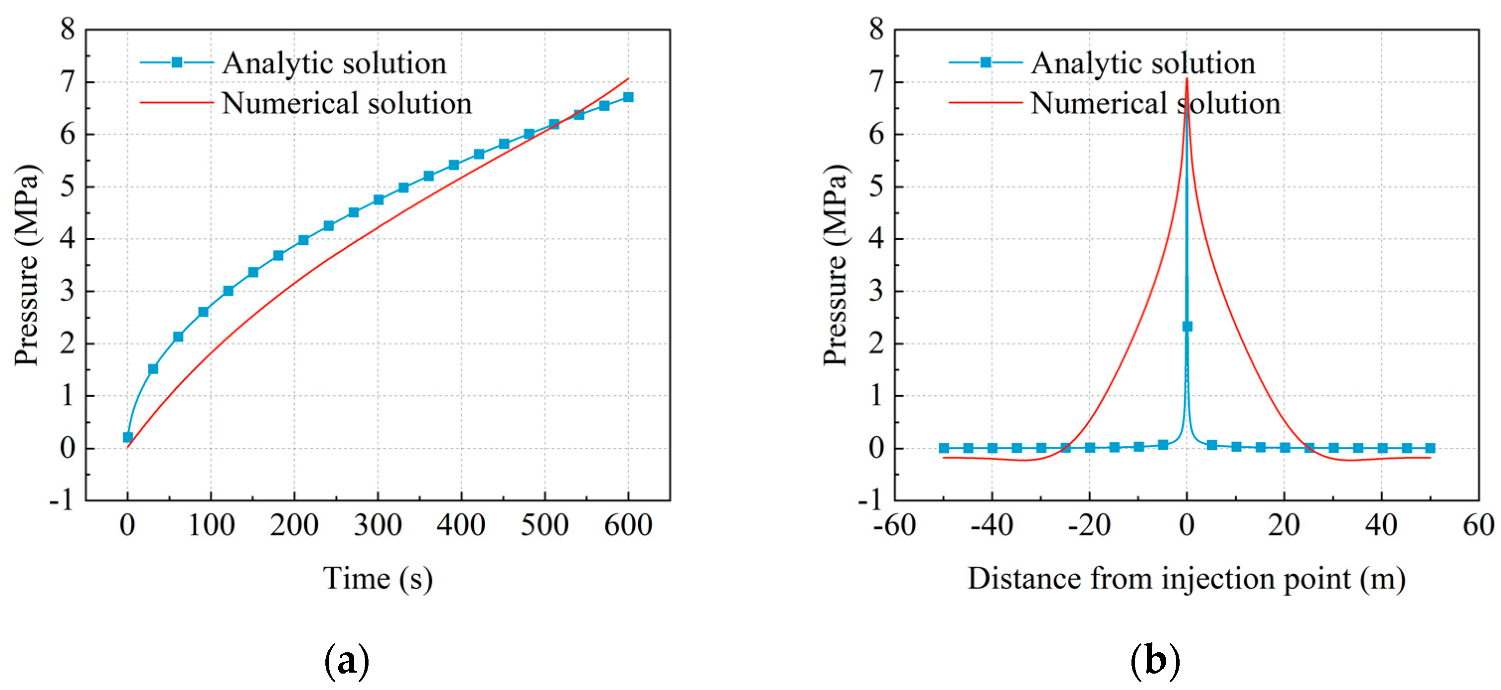
By following these initialization steps, the model aims to capture realistic stress conditions and reduce the impact of settlement displacement on the calculation of induced slip.

3.3. Verification

To verify the model, we compare the numerical and analytical solutions of pore pressure distribution after injection using Darcy’s law and Biot’s theory. The computational model is depicted in Figure 4, using the same boundary conditions and material properties as the geological model. Figure 5a shows the comparison between the numerical and analytical solutions for the maximum pore pressure. The numerical solution yields a value of 7.07 MPa, while the analytical solution yields a value of 6.71 MPa. Figure 5b presents the distribution of pore pressure at the boundary of the model obtained with the analytic and numerical solutions. The numerical model considers the enhanced permeability caused by the injection, allowing fluid pressure to diffuse more smoothly than the analytical solution. Both approaches exhibit excellent agreement, validating the reliability of the numerical simulation.

4. Results

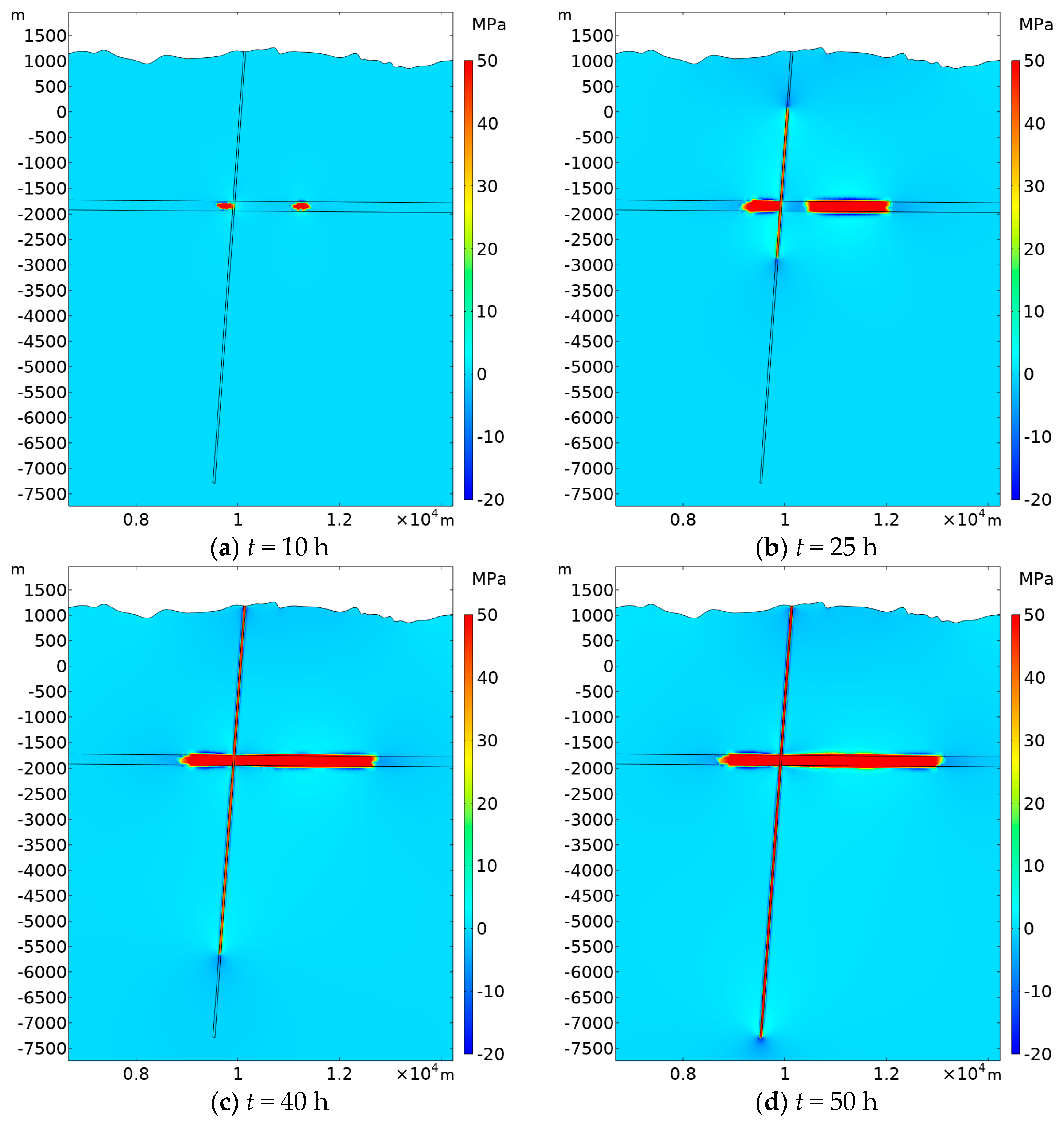
4.1. Effect of Injection on Fluid Distribution

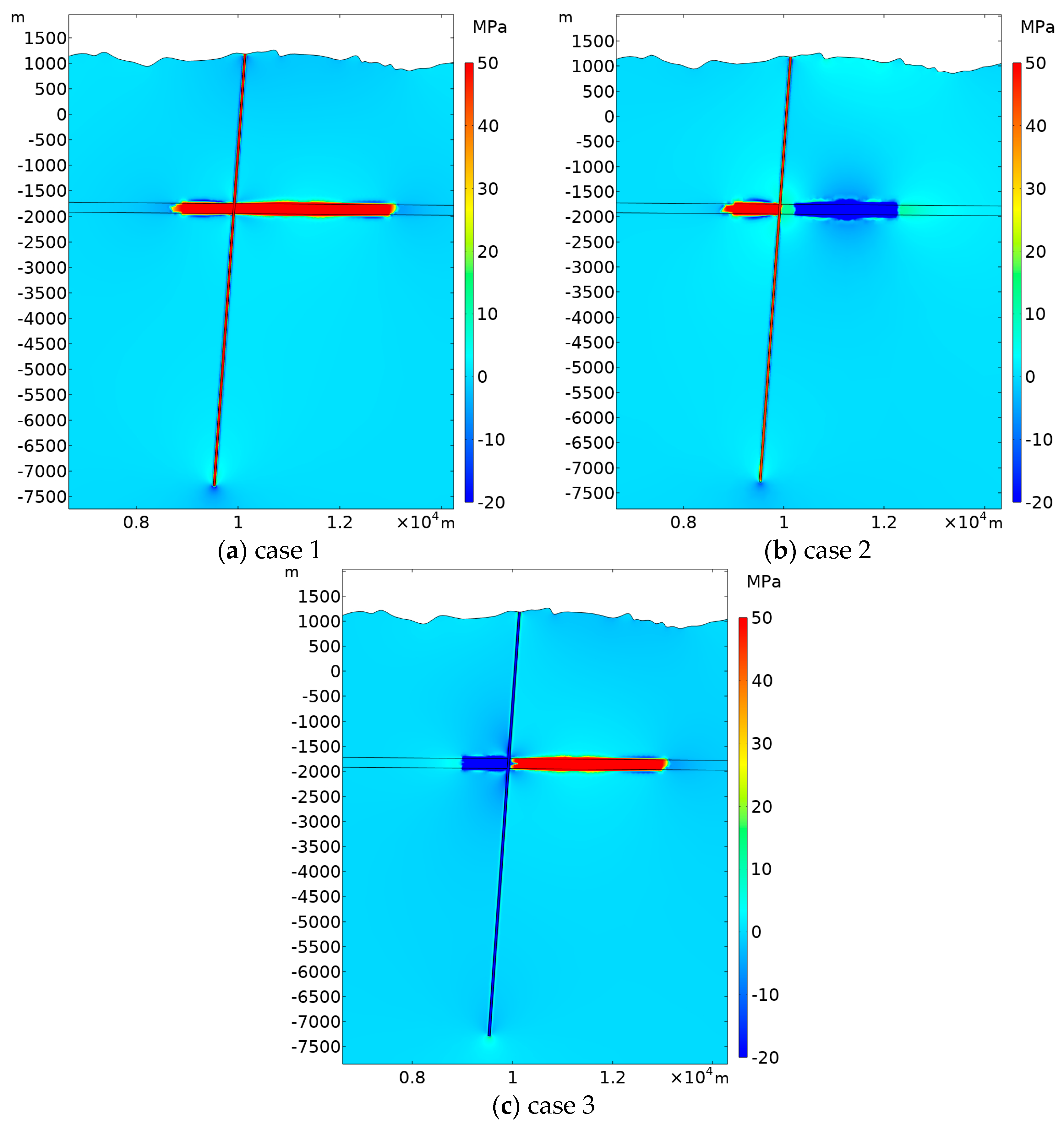
4.1.1. Pore Pressure Distribution

Figure 6 shows the pore pressure distribution in the model. High pore pressure initially appears around the injection well. Once the fluid encounters a fault, it rapidly flows along the fault, while a small amount of the fluid diffuses into the surrounding cap rock. When the fluid reaches the ground (see Figure 6c), the pore pressure rapidly diffuses along the fault to the deeper layer of the formation. At the end of the simulation, the fault is filled with fluid and the pore pressure remains stable. The fluid is stored in the fault, creating a high-pressure fluid state along it.

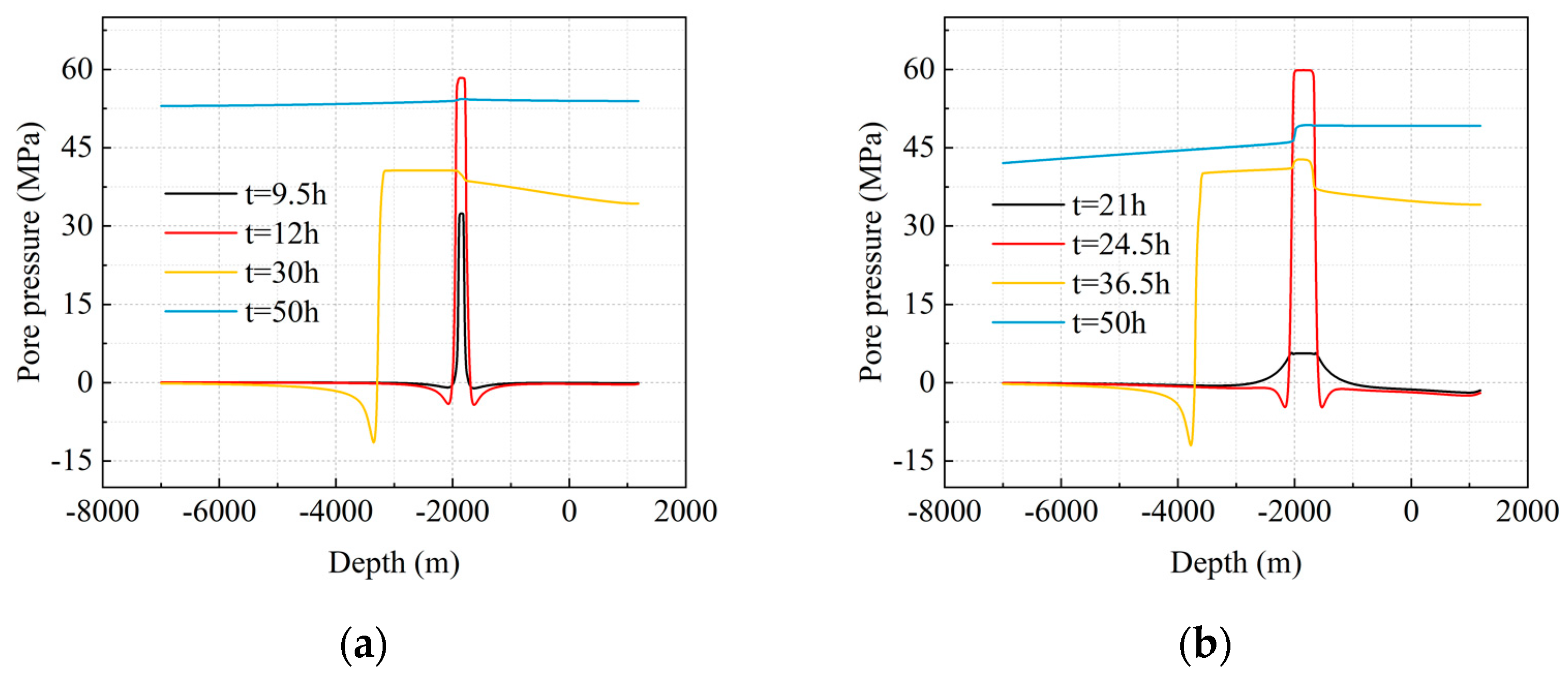
4.1.2. Evolution of Pore Pressure along the Fault

Figure 7 shows the pore pressure distribution along the fault. When d = 150 m, pore pressure diffusion along the fault is relatively slow during the pre-injection period (t = 0–9.5 h), as shown in Figure 7a. As the pore pressure within the fault reaches its peak at t = 12 h, the fluid rapidly transports along the fault [43,53]. It can be seen that a high pore pressure appears about 3000 m below the surface at t = 30 h. At the end of the simulation, the high-pressure fluid fills the entire fault and then the pore pressure inside the fault remains relatively stable, always slightly lower than the peak pressure inside the fault. When the injection well is far away from the fault (d = 750 m), the distribution characteristics of the pore pressure show similar features. In the pre-injection period, the fluid flow occurs mainly within the reservoir; thus, the pore pressure within the fault is significantly lower than that in the case of d = 150 m.

Figure 8 shows the pore pressure distribution along the fault at t = 50 h for different injection and production scenarios. When the injection well and the production well is set in the simulation, the pore pressure in the fault significantly reduces, and, in some cases, negative pore pressure even occurs. As shown in Figure 9, the distance between the production well and the fault significantly affects fluid distribution characteristics inside the fault. In case 2, where the production well is located far away from the fault, the fault acts as a conduit due to its high permeability, and fluid within the fault flows rapidly towards the production well. As a result, the pore pressure within the fault is significantly lower than that in case 1. However, if the production well is close to the fault (case 3), the presence of the production well prevents the increase in pore pressure within the fault. The production well, being close to the fault, first establishes hydraulic connectivity. Then, fluid in the surrounding rock formations is rapidly drawn in by the well. In this situation, the fault acts as a barrier for fluid flow, resulting in less noticeable pressure changes within the fault.

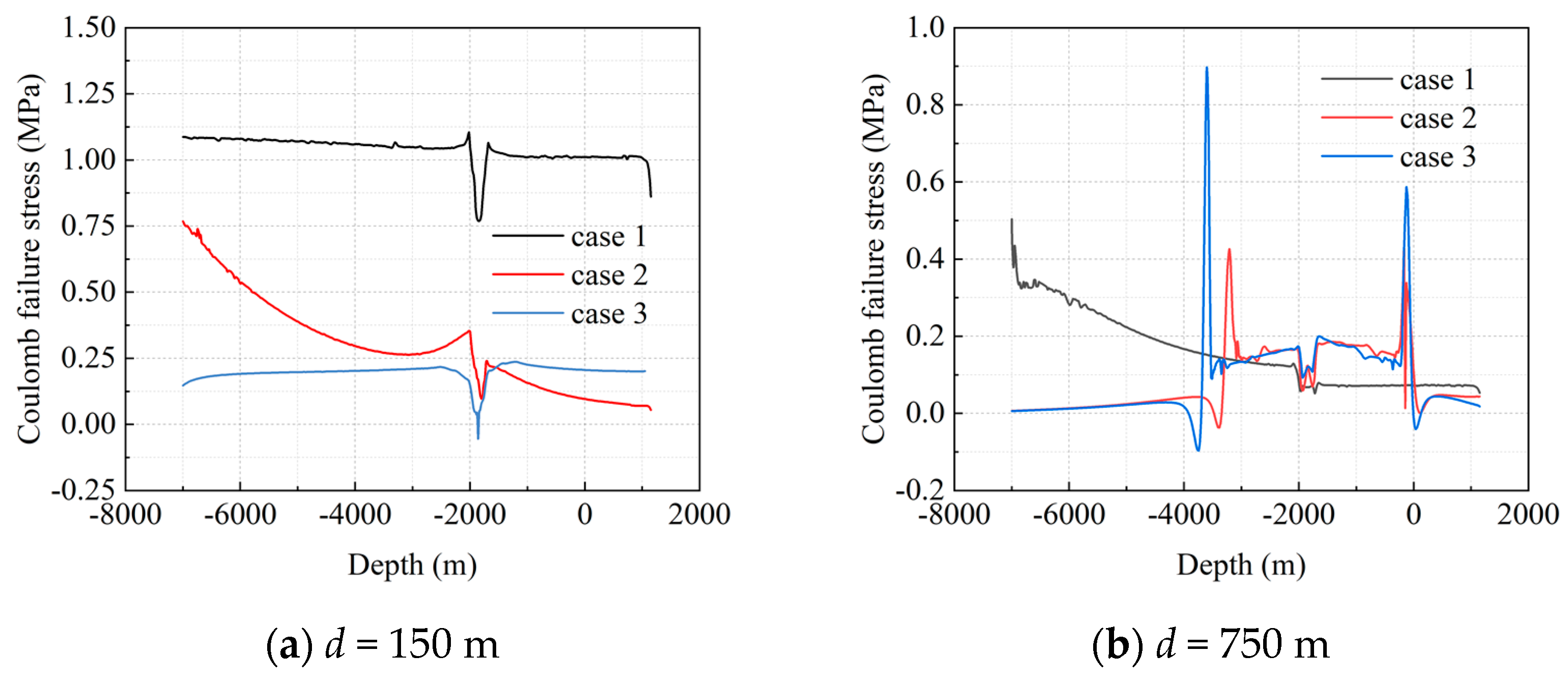
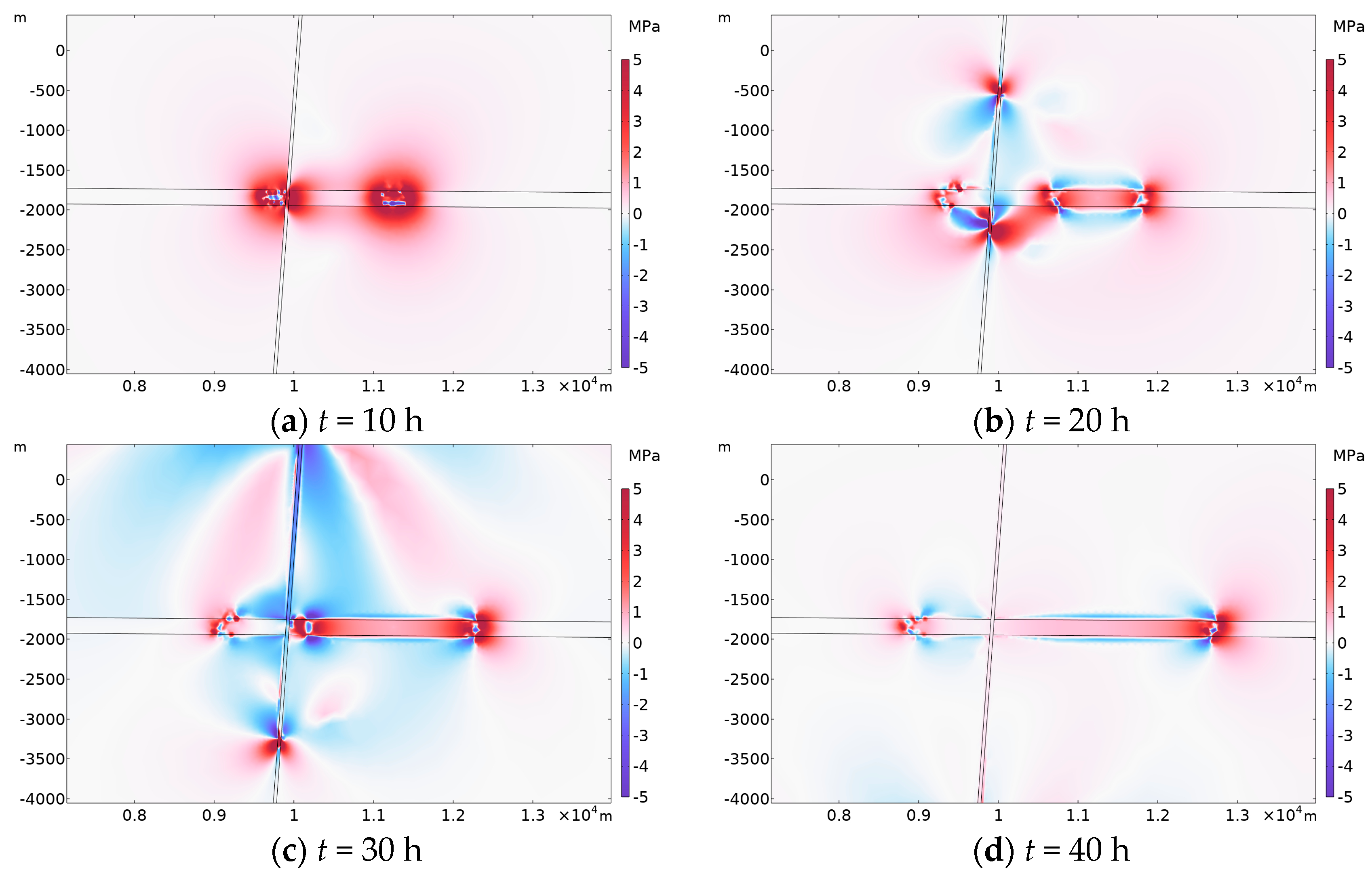
4.2. Coulomb Failure Stress (∆CFS)

Injection activities can significantly affect fault stability by generating high pore pressures along the fault. Previous research suggests that the fault could be unstable and activated when the Coulomb failure stress exceeds 0.05–0.2 MPa [2,25]. In the simulations, two different injection locations and three different injection schemes are considered (Figure 10).

When d = 150 m, the pore pressure within the fault is much higher for case 1 than other cases (Figure 10a). In case 1, high Coulomb failure stress occurs within the fault, mostly larger than 1 MPa, indicating that the fault is in a relatively active state. In case 2, where the production well is located far away from the fault, there is a significant reduction in the Coulomb failure stress, which is reduced by approximately 30% compared to case 1. The activated region in case 2 is located at the base of the fault. In case 3, where the production well is at the proximal end of the fault, most of the area on the fault is close to the activation state, which is prone to induce slip.

When d = 750 m, the activation region of the fault is much smaller than that for d = 150 m. In case 1, the value of ΔCFS is low and the possibility of fault slip is small. As shown in Figure 10b, for cases 2 and 3, it is only at the tip of the fluid flow that there is a higher risk of fault activation. The fluid-filled region returns to a relatively stable stress state. The injection and production scheme helps to reduce the possibility of fault activation.

Figure 11 illustrates the distribution of Coulomb failure stresses at different stages of fluid injection for d = 150 m. The plot shows that the Coulomb failure stress changes primarily along the wellbore, the fracture zone, and the fault. Fracturing creates a failure zone that facilitates fluid redistribution. The high-pressure fluid in the zone continues to flow, redistributing pore pressure from high-pressure to low-pressure areas. High-pressure injection causes deformation of the rock, maintaining relatively high pore pressure within the reservoir and the fault. The pore pressure stored in the fault also causes the fault to remain at a high ΔCFS level.

4.3. Induced Seismic Events

Fault reactivation caused by hydraulic fracturing is one potential factor contributing to seismic activity. When the Coulomb stress on both sides of a fault reaches a critical level, seismic activity could be induced, such as in Harrison County and Poland Township in Ohio [38,54], Alberta [55], and Pohang [5]. Since shale gas development began in 2012, the number of seismic events in Shangluo City has increased significantly. Several earthquakes exceeded the magnitude of 3. The sources of induced seismicity are usually located near the injection position, which is typically around 2 to 3 km. Injection-induced seismicity has certain characteristics compared to natural earthquakes, such as higher source intensity and shallower source depth.

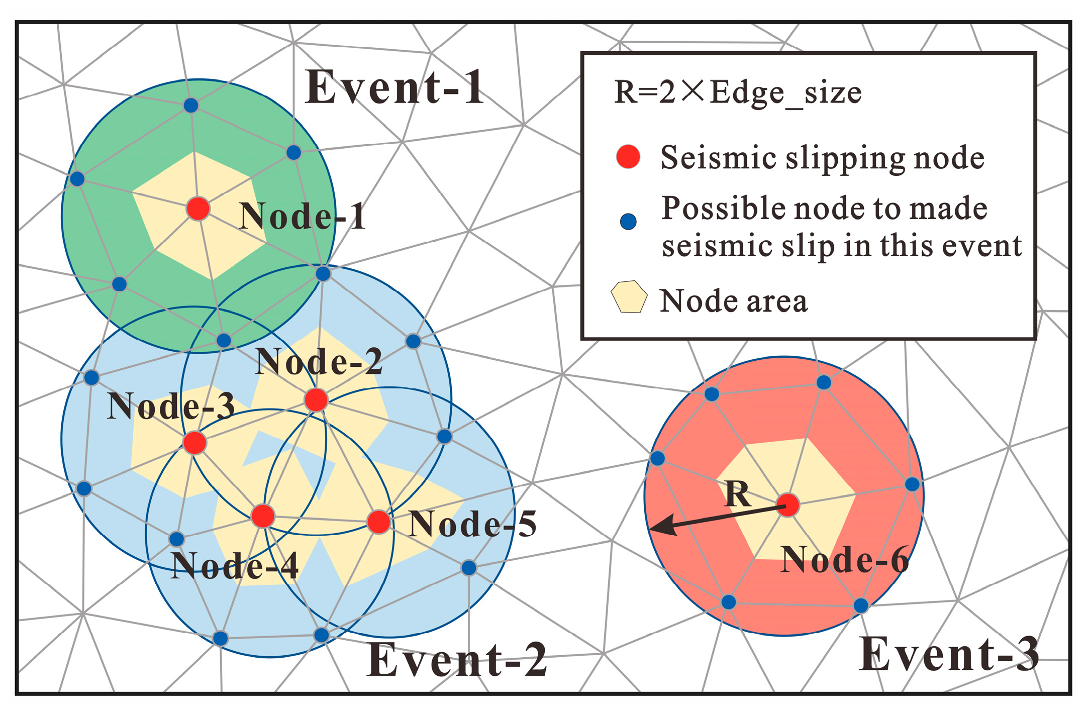
4.3.1. Calculation of Seismic Slip Events

Seismic events can be estimated based on the shear displacement and material properties. As shown in Figure 12, the vertices of the mesh triangles serve as the nodes at which events occur. Each node has an associated area of influence, which is defined as one third of the total area of all surrounding triangles. The seismic moment can be calculated with

$$M_0=GAd$$

(16)

where G is the shear modulus, A is the total area of sliding nodes in an earthquake event, and d is the average value of plastic slip of all slip nodes.

Equation (16) only considers shear failure and ignores seismic events caused by tensile failure. It may overestimate the proportion of large seismic events in the model, as some slip behavior does not result in seismic activity. Therefore, only the nodes that experience seismic slip should be counted as seismic events. Each node is treated as an individual event with a radius of R. Slip nodes within this range can be calculated as part of the same event; otherwise, they are considered to be separate events.

The moment magnitude can be calculated with [44]

$$M_w=\frac{2}{3}{\mathit{log}}_{10}{M}_0-9.1$$

(17)

Injection-induced fault activity can be classified into three categories on the basis of slip velocity: creep and slow slip, aseismic slip, and seismic slip [3]. In this study, slip nodes are considered to be seismic slip only if they satisfy two conditions: (1) the Coulomb failure stress is greater than 0.2 MP, and (2) the slip velocity is greater than 0.2 mm/s. The ΔCFS threshold guarantees that rock failure occurs within the defined area, while the critical velocity threshold prevents slow creep and aseismic slip [27,56].

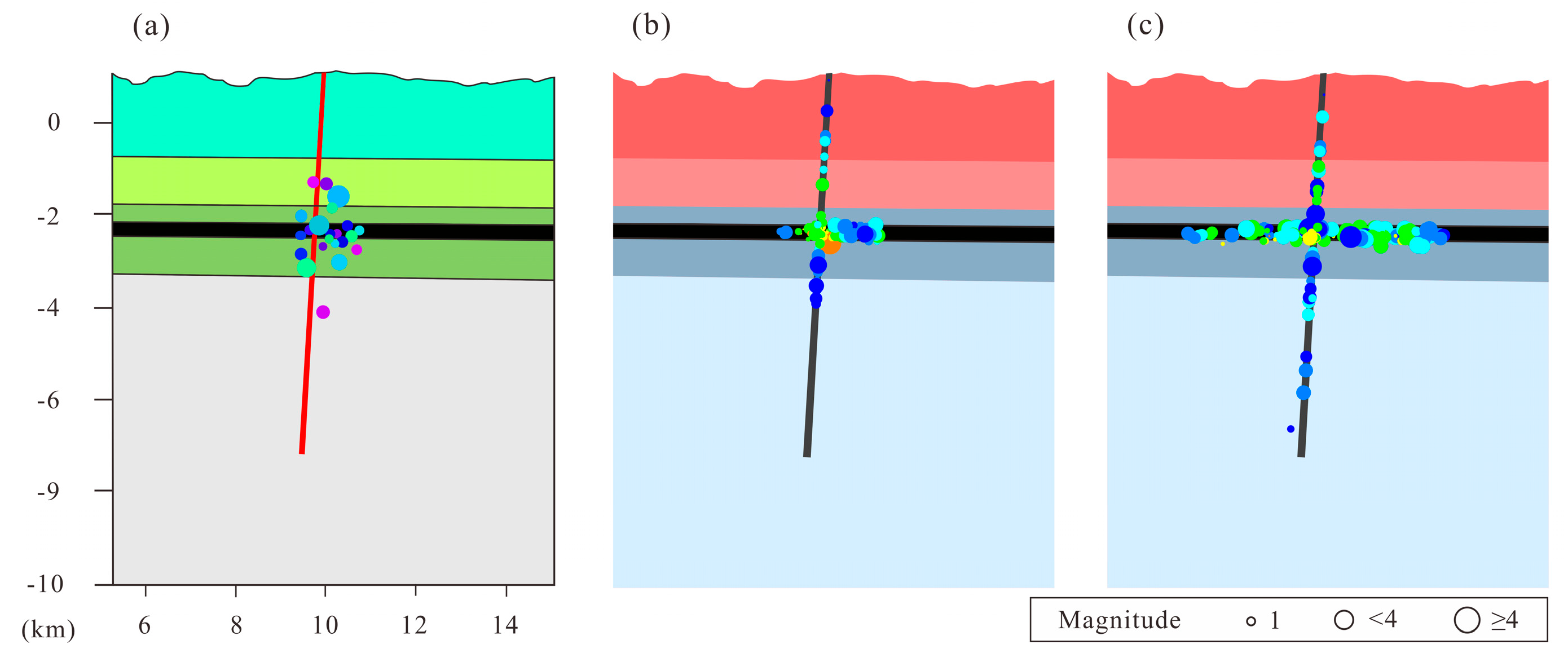
4.3.2. Distribution of Seismic Slip Events

Figure 13 presents simulated seismic events caused by fluid injections. The results show a similarity between the distribution of seismic events and that of pore pressure. During the initial stage of injection, the magnitude of seismic events is relatively small (mostly smaller than 2). Typically, micro-seismic events are first observed near the injection well after 4–6 h of injection. However, there is a significant increase in seismic activity after a period of fluid injection as the fluid enters the fault. The majority of these events are earthquakes with Mw = 2–3, but some can even reach Mw > 4. Seismic activity first occurs near the injection well and then spreads to both sides of the fault. Seismic events occur at the interface between the reservoir and the caprock due to differences in material properties. The reservoir rock is subject to damage due to high-pressure fluid. In contrast, the hydraulic transformation of caprock with low permeability and good rock properties is negligible, resulting in a significant velocity difference of deformation at the reservoir/caprock interface. As a result, seismic events are mostly concentrated at the interface.

5. Discussion

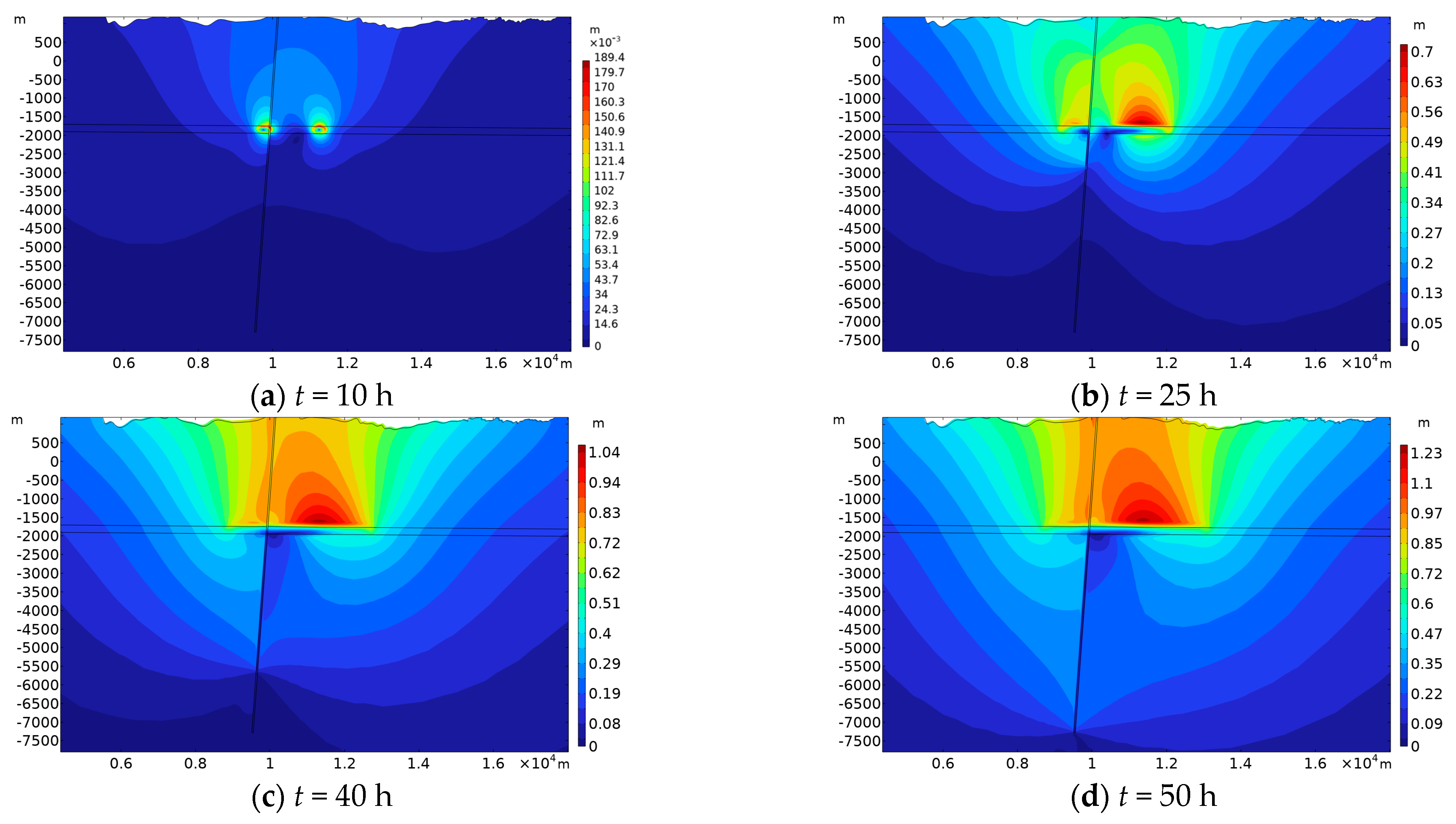
5.1. Effects of Injection on Formation Deformation

When the fracturing fluid is injected into the target reservoir, it will inevitably produce pore pressure accumulation, effective stress change, and reservoir deformation [58,59]. To prevent the deformation of the reservoir from being transmitted to the surface and causing damage to ground facilities, it is necessary to consider the ground uplift caused by the injection of fracturing fluid. Under the influence of high-pressure fluid injection, the rock mass above the reservoir deforms, causing an upward movement [60]. Figure 14 shows that displacement mainly concentrates near the injection well and the high-permeability fault.

5.2. Fault Slip

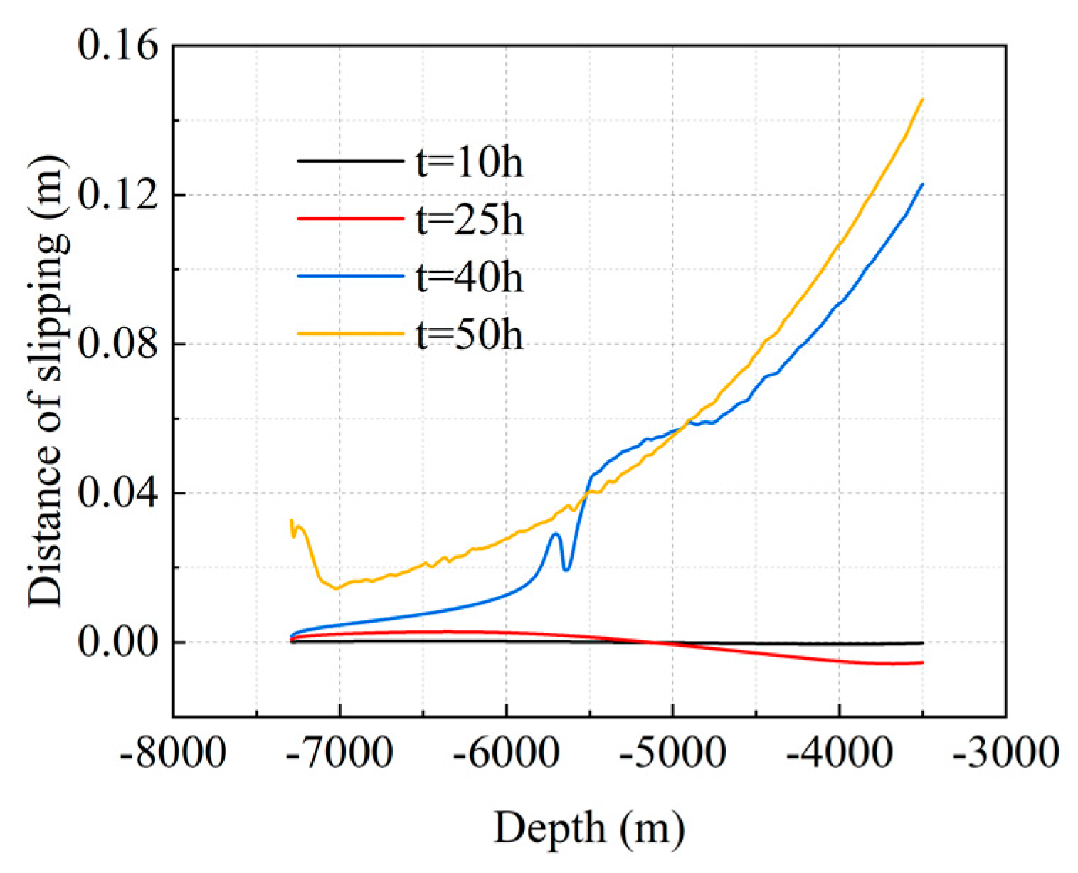
5.2.1. Effect of Injection Time

Figure 15 shows the variation in fault slip with time. At the beginning, slippage is small. At t = 40 h, a significant upward shift occurs. At the end of the simulation, the fault is fully filled with fluid and there is relatively stable slippage between the upper and lower walls of the fault, indicating a trend of reverse fault slippage. With a maximum distance of slippage of about 0.14 m, the slip near the surface is greater than that in the deep rock layer.

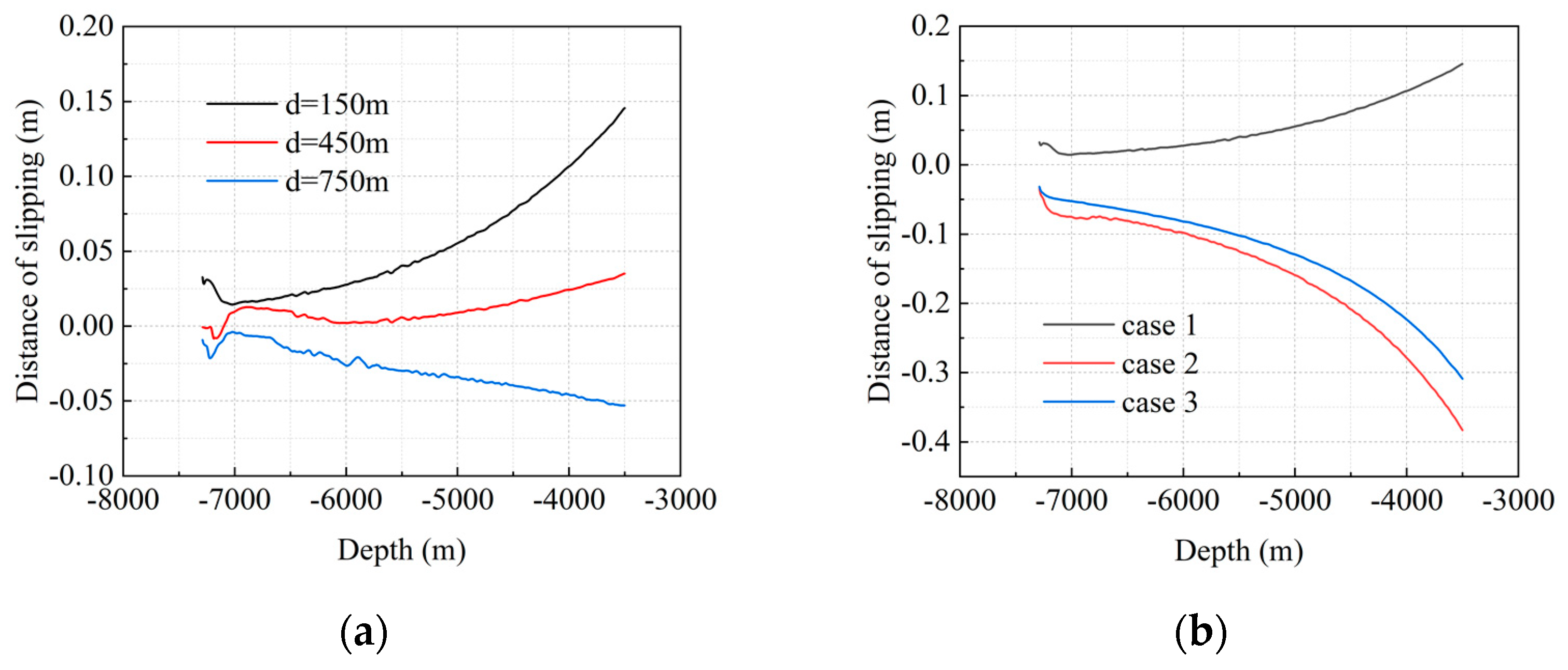
5.2.2. Effect of Injection Rate

Injection rate is a crucial factor that affects the efficiency of hydraulic fracturing and directly impacts the extent of reservoir stimulation. Higher injection pressure often results in better reservoir modification. However, it also increases the probability of induced fault slip. Figure 16 shows that the effect of injection rate on the fault is not significant when the injection rate is less than 7.5 m³/h. As the injection rate increases, the affected area within the fault expands noticeably. Due to the injection well’s proximity to the hanging wall of the fault, the hanging wall experiences larger relative displacements compared to the footwall. When the injection rate is 22.5 m³/h, the slippage increases by approximately 25%. Therefore, an appropriate reduction in the injection rate could minimize the occurrence of fault slip without significantly compromising the effectiveness of reservoir modification.

5.2.3. Effect of Injection–Production Schemes

Figure 17a shows the impact of injection–production schemes on slip mechanisms. For the cases with d = 150 m and 450 m, where the injection well is closer to the fault, a significant velocity component on the hanging wall results in a reverse fault-slip state. When the distance of the two injection wells to the fault is the same (d = 750 m), the injection on the footwall is dominant, facilitating fluid flow towards the lower portion of the fault. The hanging wall rock mass undergoes downward sliding, resulting in a negative slip difference, which indicates a normal fault behavior.

(1) Case 1 with two injection wells; (2) case 2 with one injection well located on the hanging wall of the fault and one production well located on the footwall of the fault; and (3) case 3 with one injection well located on the footwall of the fault and one production well located on the hanging wall of the fault.

For cases 2 and 3, where one injection well and one production well are set, slip distance of −0.38 m and −0.31 m occurs, respectively (Figure 17b). If the production well is far from the fault (case 2), the fault is in a conduit state and most of the fluid migrates through the fault to the production well. This weakens the movement trend of the hanging wall of the fault. When the production well is located close to the fault (case 3), the surrounding rock mass contracts towards the well, resulting in a relatively slow movement rate. In summary, due to the presence of the production well, the hanging wall motion component is reduced, resulting in a normal fault-slip mechanism.

6. Conclusions

This study presents a fully coupled numerical investigation of seismic events and fault-slip mechanisms in the Shangluo region of Sichuan province, China. The distribution of fluid pressure and Coulomb failure stress was simulated using FEM. The findings are listed as follows:

(1)

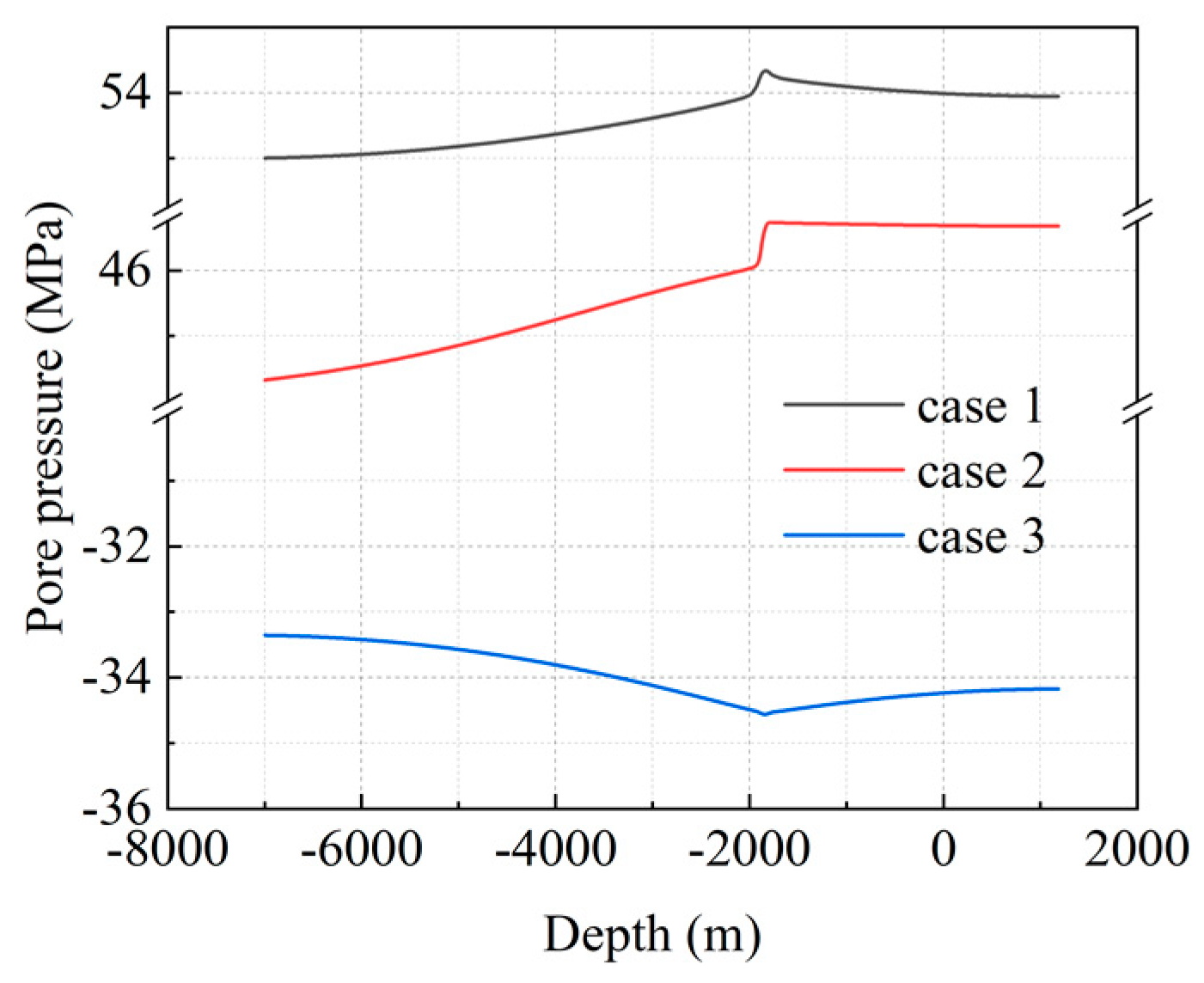
High-permeability faults display three distinct behaviors under different production schemes: barrier, fluid transport channel, and conduit channel. The faults act as conduits in the absence of producing wells. Where the production well is located far away from the fault, the fault acts as a conduit channel. If the production well is close to the fault, the fault acts as a barrier for fluid flow.

(2)

The migration of high-pressure fluid in the formation is closely related to the degree of rock fracturing. This leads to most of the area on the fault close to the activation state. As the fluid distribution within the fault rock mass tends to be stable, the fault can return to a relatively stable stress state.

(3)

The results show that the displacement mainly occurs near the injection well and the fault. The production time and injection rate affect the distance of fault slip, and the fault slip near the surface is greater than in other places. The injection production scenarios could influence the fault-slip mechanism, resulting in a normal fault or reverse fault.

These results could help to understand seismic events and fault behavior in the Shangluo region and provide valuable insights for reservoir stimulations and seismic hazard assessments in similar geological settings.

References

1. Foulger, G.R.; Wilson, M.P.; Gluyas, J.G.; Julian, B.R.; Davies, R.J. Global review of human-induced earthquakes. Earth-Sci. Rev. 2018, 178, 438–514. [Google Scholar] [CrossRef]
2. Hui, G.; Chen, S.; Chen, Z.; Gu, F. An integrated approach to characterize hydraulic fracturing-induced seismicity in shale reservoirs. J. Pet. Sci. Eng. 2021, 196, 107624. [Google Scholar] [CrossRef]
3. Wu, W.; Lu, D.; Elsworth, D. Fluid injection-induced fault slip during unconventional energy development: A review. Energy Rev. 2022, 1, 100007. [Google Scholar] [CrossRef]
4. Dong, K.; Liu, N.; Chen, Z.; Huang, R.; Ding, J.; Niu, G. Geomechanical analysis on casing deformation in Longmaxi shale formation. J. Pet. Sci. Eng. 2019, 177, 724–733. [Google Scholar] [CrossRef]
5. Wassing, B.B.T.; Gan, Q.; Candela, T.; Fokker, P.A. Effects of fault transmissivity on the potential of fault reactivation and induced seismicity: Implications for understanding induced seismicity at Pohang EGS. Geothermics 2021, 91, 101976. [Google Scholar] [CrossRef]
6. Gan, Q.; Feng, Z.; Zhou, L.; Li, H.; Liu, J.; Elsworth, D. Down-dip circulation at the united downs deep geothermal power project maximizes heat recovery and minimizes seismicity. Geothermics 2021, 96, 102204. [Google Scholar] [CrossRef]
7. Schultz, R.; Skoumal, R.J.; Brudzinski, M.R.; Eaton, D.; Baptie, B.; Ellsworth, W. Hydraulic Fracturing-Induced Seismicity. Rev. Geophys. 2020, 58, e2019RG000695. [Google Scholar] [CrossRef]
8. Farghal, N.; Zoback, M. Utilizing Ant-tracking to Identify Slowly Slipping Faults in the Barnett Shale. In Proceedings of the 2nd URteC 1922263, Denver, CO, USA, 25–27 August 2014. [Google Scholar]
9. Eyre, T.S.; Eaton, D.W.; Garagash, D.I.; Zecevic, M.; Venieri, M.; Weir, R.; Lawton, D.C. The role of aseismic slip in hydraulic fracturing–induced seismicity. Sci. Adv. 2019, 5, eaav7172. [Google Scholar] [CrossRef] [PubMed]
10. Meng, H.; Ge, H.; Yao, Y.; Shen, Y.; Wang, J.; Bai, J.; Zhang, Z. A new insight into casing shear failure induced by natural fracture and artificial fracture slip. Eng. Fail. Anal. 2022, 137, 106287. [Google Scholar] [CrossRef]
11. Xi, Y.; Li, J.; Liu, G.; Li, J.; Jiang, J. Mechanisms and Influence of Casing Shear Deformation near the Casing Shoe, Based on MFC Surveys during Multistage Fracturing in Shale Gas Wells in Canada. Energies 2019, 12, 372. [Google Scholar] [CrossRef]
12. Eyre, T.S.; Samsonov, S.; Feng, W.; Kao, H.; Eaton, D.W. InSAR data reveal that the largest hydraulic fracturing-induced earthquake in Canada, to date, is a slow-slip event. Sci. Rep. 2022, 12, 2043. [Google Scholar] [CrossRef]
13. Xu, B.; Hu, J.; Hu, T.; Wang, F.; Luo, K.; Wang, Q.; He, X. Quantitative assessment of seismic risk in hydraulic fracturing areas based on rough set and Bayesian network: A case analysis of Changning shale gas development block in Yibin City, Sichuan Province, China. J. Pet. Sci. Eng. 2021, 200, 108226. [Google Scholar] [CrossRef]
14. Hu, J.; Xu, B.; Chen, Z.; Zhang, H.; Cao, J.; Wang, Q. Hazard and risk assessment for hydraulic fracturing induced seismicity based on the Entropy-Fuzzy-AHP method in Southern Sichuan Basin, China. J. Nat. Gas Sci. Eng. 2021, 90, 103908. [Google Scholar] [CrossRef]
15. Xi, Y.; Jiang, J.; Li, J.; Li, H.; Gao, D. Research on the influence of strike-slip fault slippage on production casing and control methods and engineering application during multistage fracturing in deep shale gas wells. Energy Rep. 2021, 7, 2989–2998. [Google Scholar] [CrossRef]
16. Kruszewski, M.; Montegrossi, G.; Balcewicz, M.; de Los Angeles Gonzalez de Lucio, G.; Igbokwe, O.A.; Backers, T.; Saenger, E.H. 3D in situ stress state modelling and fault reactivation risk exemplified in the Ruhr region (Germany). Geomech. Energy Environ. 2022, 32, 100386. [Google Scholar] [CrossRef]
17. Huang, Y.; Lei, X.; Ma, S. Numerical study of the role of localized stress perturbations on fault slip: Insights for injection-induced fault reactivation. Tectonophysics 2021, 819, 229105. [Google Scholar] [CrossRef]
18. Eyinla, D.S.; Oladunjoye, M.A.; Gan, Q.; Olayinka, A.I. Fault reactivation potential and associated permeability evolution under changing injection conditions. Petroleum 2021, 7, 282–293. [Google Scholar] [CrossRef]
19. Verdon, J.P.; Rodríguez-Pradilla, G. Assessing the variability in hydraulic fracturing-induced seismicity occurrence between North American shale plays. Tectonophysics 2023, 859, 229898. [Google Scholar] [CrossRef]
20. Wasantha, P.L.P.; Konietzky, H. Fault reactivation and reservoir modification during hydraulic stimulation of naturally-fractured reservoirs. J. Nat. Gas Sci. Eng. 2016, 34, 908–916. [Google Scholar] [CrossRef]
21. Gan, Q.; Lei, Q. Induced fault reactivation by thermal perturbation in enhanced geothermal systems. Geothermics 2020, 86, 101814. [Google Scholar] [CrossRef]
22. Lv, Y.; Yuan, C.; Zhu, X.; Gan, Q.; Li, H. THMD analysis of fluid injection-induced fault reactivation and slip in EGS. Geothermics 2022, 99, 102303. [Google Scholar] [CrossRef]
23. Zhang, H.; Tong, H.; Zhang, P.; He, Y.; Liu, Z.; Huang, Y. How can casing deformation be prevented during hydraulic fracturing of shale gas?—A case study of the Weiyuan area in Sichuan, China. Geoenergy Sci. Eng. 2023, 221, 111251. [Google Scholar] [CrossRef]
24. Niemeijer, A.; Marone, C.; Elsworth, D. Frictional strength and strain weakening in simulated fault gouge: Competition between geometrical weakening and chemical strengthening. J. Geophys. Res. Solid Earth 2010, 115. [Google Scholar] [CrossRef]
25. An, M.; Zhang, F.; Dontsov, E.; Elsworth, D.; Zhu, H.; Zhao, L. Stress perturbation caused by multistage hydraulic fracturing: Implications for deep fault reactivation. Int. J. Rock Mech. Min. Sci. 2021, 141, 104704. [Google Scholar] [CrossRef]
26. Im, K.; Elsworth, D.; Guglielmi, Y.; Mattioli, G.S. Geodetic imaging of thermal deformation in geothermal reservoirs—Production, depletion and fault reactivation. J. Volcanol. Geotherm. Res. 2017, 338, 79–91. [Google Scholar] [CrossRef]
27. Yin, Z.; Huang, H.; Zhang, F.; Zhang, L.; Maxwell, S. Three-dimensional distinct element modeling of fault reactivation and induced seismicity due to hydraulic fracturing injection and backflow. J. Rock Mech. Geotech. Eng. 2020, 12, 752–767. [Google Scholar] [CrossRef]
28. Zhang, F.; Cao, S.; An, M.; Zhang, C.; Elsworth, D. Friction and stability of granite faults in the Gonghe geothermal reservoir and implications for injection-induced seismicity. Geothermics 2023, 112, 102730. [Google Scholar] [CrossRef]
29. Volpe, G.; Pozzi, G.; Collettini, C.; Spagnuolo, E.; Achtziger-Zupančič, P.; Zappone, A.; Aldega, L.; Meier, M.A.; Giardini, D.; Cocco, M. Laboratory simulation of fault reactivation by fluid injection and implications for induced seismicity at the BedrettoLab, Swiss Alps. Tectonophysics 2023, 862, 229987. [Google Scholar] [CrossRef]
30. Liu, K.; Taleghani, A.D.; Gao, D. Calculation of hydraulic fracture induced stress and corresponding fault slippage in shale formation. Fuel 2019, 254, 115525. [Google Scholar] [CrossRef]
31. Huang, N.; Liu, R.; Jiang, Y.; Cheng, Y.; Li, B. Shear-flow coupling characteristics of a three-dimensional discrete fracture network-fault model considering stress-induced aperture variations. J. Hydrol. 2019, 571, 416–424. [Google Scholar] [CrossRef]
32. Wang, L.; Golfier, F.; Tinet, A.-J.; Chen, W.; Vuik, C. An efficient adaptive implicit scheme with equivalent continuum approach for two-phase flow in fractured vuggy porous media. Adv. Water Resour. 2022, 163, 104186. [Google Scholar] [CrossRef]
33. Pan, W.; Zhang, Z.; Wang, S.; Lei, Q. Earthquake-induced fracture displacements and transmissivity changes in a 3D fracture network of crystalline rock for spent nuclear fuel disposal. J. Rock Mech. Geotech. Eng. 2023, 15, 2313–2329. [Google Scholar] [CrossRef]
34. Park, J.-W.; Guglielmi, Y.; Graupner, B.; Rutqvist, J.; Kim, T.; Park, E.-S.; Lee, C. Modeling of fluid injection-induced fault reactivation using coupled fluid flow and mechanical interface model. Int. J. Rock Mech. Min. Sci. 2020, 132, 104373. [Google Scholar] [CrossRef]
35. Eyinla, D.S. Modelling of fault reactivation mechanisms and associated induced seismicity in rocks with different elastic materials. Pet. Res. 2022, 7, 91–105. [Google Scholar] [CrossRef]
36. Zhou, S.; Zhuang, X.; Rabczuk, T. Phase-field modeling of fluid-driven dynamic cracking in porous media. Comput. Methods Appl. Mech. Eng. 2019, 350, 169–198. [Google Scholar] [CrossRef]
37. Santillán, D.; Juanes, R.; Cueto-Felgueroso, L. Phase Field Model of Hydraulic Fracturing in Poroelastic Media: Fracture Propagation, Arrest, and Branching Under Fluid Injection and Extraction. J. Geophys. Res. Solid Earth 2018, 123, 2127–2155. [Google Scholar] [CrossRef]
38. Segall, P.; Lu, S. Injection-induced seismicity: Poroelastic and earthquake nucleation effects. J. Geophys. Res. Solid Earth 2015, 120, 5082–5103. [Google Scholar] [CrossRef]
39. Wang, L.; Yin, Z.-Y.; Han, G.; Yu, M. Toward temporal evolution of consolidation in fluid-saturated poroelastic media with various permeable conditions. Comput. Geotech. 2023, 156, 105273. [Google Scholar] [CrossRef]
40. Biot, M.A. General Theory of Three—Dimensional Consolidation. J. Appl. Phys. 2004, 12, 155–164. [Google Scholar] [CrossRef]
41. Wang, L.; Chen, W.; Vuik, C. Hybrid-dimensional modeling for fluid flow in heterogeneous porous media using dual fracture-pore model with flux interaction of fracture–cavity network. J. Nat. Gas Sci. Eng. 2022, 100, 104450. [Google Scholar] [CrossRef]
42. Rutqvist, J.; Noorishad, J.; Tsang, C.F.; Stephansson, O. Determination of fracture storativity in hard rocks using high-pressure injection testing. Water Resour. Res. 1998, 34, 2551–2560. [Google Scholar] [CrossRef]
43. Cappa, F.; Rutqvist, J. Modeling of coupled deformation and permeability evolution during fault reactivation induced by deep underground injection of CO2. Int. J. Greenh. Gas Control 2011, 5, 336–346. [Google Scholar] [CrossRef]
44. Rutqvist, J.; Rinaldi, A.P.; Cappa, F.; Moridis, G.J. Modeling of fault reactivation and induced seismicity during hydraulic fracturing of shale-gas reservoirs. J. Pet. Sci. Eng. 2013, 107, 31–44. [Google Scholar] [CrossRef]
45. Kim, S.; Hosseini, S.A. Geological CO2 storage: Incorporation of pore-pressure/stress coupling and thermal effects to determine maximum sustainable pressure limit. Energy Procedia 2014, 63, 3339–3346. [Google Scholar] [CrossRef]
46. Cappa, F.; Guglielmi, Y.; Nussbaum, C.; Birkholzer, J. On the Relationship Between Fault Permeability Increases, Induced Stress Perturbation, and the Growth of Aseismic Slip During Fluid Injection. Geophys. Res. Lett. 2018, 45, 11012–11020. [Google Scholar] [CrossRef]
47. Rutqvist, J.; Stephansson, O. The role of hydromechanical coupling in fractured rock engineering. Hydrogeol. J. 2003, 11, 7–40. [Google Scholar] [CrossRef]
48. Catalli, F.; Meier, M.A.; Wiemer, S. The role of Coulomb stress changes for injection—Induced seismicity: The Basel enhanced geothermal system. Geophys. Res. Lett. 2013, 40, 72–77. [Google Scholar] [CrossRef]
49. Zhan, Z.Y. Study on Controlling Factors of Marine Shale Gas Dispersion in South China: A Case Study of Southern Margin of Sichuan Basin; China University of Petroleum: Beijing, China, 2019. [Google Scholar]
50. Pereira, L.C.; Guimarães, L.J.N.; Horowitz, B.; Sánchez, M. Coupled hydro-mechanical fault reactivation analysis incorporating evidence theory for uncertainty quantification. Comput. Geotech. 2014, 56, 202–215. [Google Scholar] [CrossRef]
51. Sun, C.; Shen, F.; Wen, Z.; Zhang, Y.; Scarselli, N.; Li, S.; Yu, Y.; Wu, G. Seismic analysis of fault damage zones in the northern Tarim Basin (NW China): Implications for growth of ultra-deep fractured reservoirs. J. Asian Earth Sci. 2023, 255, 105778. [Google Scholar] [CrossRef]
52. Mortezaei, K.; Vahedifard, F. Multi-scale simulation of thermal pressurization of fault fluid under CO2 injection for storage and utilization purposes. Int. J. Rock Mech. Min. Sci. 2017, 98, 111–120. [Google Scholar] [CrossRef]
53. Jia, Y.; Wu, W.; Kong, X.-Z. Injection-induced slip heterogeneity on faults in shale reservoirs. Int. J. Rock Mech. Min. Sci. 2020, 131, 104363. [Google Scholar] [CrossRef]
54. Fasola, S.L.; Brudzinski, M.R.; Skoumal, R.J.; Langenkamp, T.; Currie, B.S.; Smart, K.J. Hydraulic Fracture Injection Strategy Influences the Probability of Earthquakes in the Eagle Ford Shale Play of South Texas. Geophys. Res. Lett. 2019, 46, 12958–12967. [Google Scholar] [CrossRef]
55. Hui, G.; Chen, Z.; Schultz, R.; Chen, S.; Song, Z.; Zhang, Z.; Song, Y.; Wang, H.; Wang, M.; Gu, F. Intricate unconventional fracture networks provide fluid diffusion pathways to reactivate pre-existing faults in unconventional reservoirs. Energy 2023, 282, 128803. [Google Scholar] [CrossRef]
56. Zhang, F.; Mack, M. Integrating fully coupled geomechanical modeling with microsesmicity for the analysis of refracturing treatment. J. Nat. Gas Sci. Eng. 2017, 46, 16–25. [Google Scholar] [CrossRef]
57. Lei, X.; Huang, D.; Su, J.; Jiang, G.; Wang, X.; Wang, H.; Guo, X.; Fu, H. Fault reactivation and earthquakes with magnitudes of up to Mw4.7 induced by shale-gas hydraulic fracturing in Sichuan Basin, China. Sci. Rep. 2017, 7, 7971. [Google Scholar] [CrossRef]
58. Rutqvist, J. Status of the TOUGH-FLAC simulator and recent applications related to coupled fluid flow and crustal deformations. Comput. Geosci. 2011, 37, 739–750. [Google Scholar] [CrossRef]
59. Jun, S.; Song, Y.; Wang, J.; Weijermars, R. Formation uplift analysis during geological CO2-Storage using the Gaussian pressure transient method: Krechba (Algeria) validation and South Korean case studies. Geoenergy Sci. Eng. 2023, 221, 211404. [Google Scholar] [CrossRef]
60. Siriwardane, H.J.; Gondle, R.K.; Varre, S.B.; Bromhal, G.S.; Wilson, T.H. Geomechanical response of overburden caused by CO2 injection into a depleted oil reservoir. J. Rock Mech. Geotech. Eng. 2016, 8, 860–872. [Google Scholar] [CrossRef]
Figure 1. Schematic representation of the Coulomb failure stress (CFS): (a) shear failure diagram before injection; (b) shear failure diagram after injection; (c) Mohr circles with the Coulomb criteria showing failure envelopes. In (c), black circle represents a stable state and red circle represents shear failure. If the pore pressure P increases due to fluid injection, the circle will move to the left and reach the failure envelope.
Energies 17 01614 g001
Figure 2. Two-dimensional geological model of the study area.   T 1 ,   P ,   Z , and Pt2-3 represent limestone formation, and S represents shale reservoir.
Energies 17 01614 g002
Figure 3. Schematic representation of the injection/production schemes: (a) three different distances between the injection well and the fault, where the spacing D between two wells in each case is fixed at 1500 m; (b) three injection/production scenarios used in the simulations.
Energies 17 01614 g003
Figure 4. Validation model.
Energies 17 01614 g004
Figure 5. Results of analytical and numerical solutions. (a) Variation of pore pressure with time at the monitoring point; (b) pore pressure distribution along the monitoring line after 600 s of fluid injection.
Energies 17 01614 g005
Figure 6. Distribution of pore pressure during fluid injection: (a) t = 10 h, (b) t = 25 h, (c) t = 40 h, and (d) t = 50 h.
Energies 17 01614 g006
Figure 7. Variation of pore pressure along the fault with time: (a) d = 150 m; (b) d = 750 m.
Energies 17 01614 g007
Figure 8. Pore pressure distribution along the fault at t = 50 h for different scenarios.
Energies 17 01614 g008
Figure 9. Pore pressure distribution for different injection–production scenarios when d = 150 m: (a) case 1, (b) case 2 and (c) case 3.
Energies 17 01614 g009
Figure 10. Variation of Coulomb failure stresses along the fault at t = 50 h: (a) d = 150 m; (b) d = 750 m.
Energies 17 01614 g010
Figure 11. Coulomb failure stress distribution at different time for d = 150 m: (a) t = 10 h, (b) t = 20 h, (c) t = 30 h, and (d) t = 40 h.
Energies 17 01614 g011
Figure 12. Seismic event estimation method.
Energies 17 01614 g012
Figure 13. Seismic events. (a) Actual seismic events in Shangluo, Sichuan, since 1 January 2015, where seismic symbols are colored by date and scaled by magnitude [57]; (b) the distribution of associated seismic events after 20 h of fluid injection; (c) the distribution of seismic events after 50 h of fluid injection.
Energies 17 01614 g013
Figure 14. Distribution of displacement at different time: (a) t = 10 h, (b) t = 25 h, (c) t = 40 h, and (d) t = 50 h.
Energies 17 01614 g014
Figure 15. Cumulative slippage along the fault at different time.
Energies 17 01614 g015
Figure 16. Cumulative slippage along the fault for different injection rates.
Energies 17 01614 g016
Figure 17. Slippage along the fault for (a) different spacing between the wells and the fault, and (b) different production scenarios.
Energies 17 01614 g017