Integrating Compressed CO₂ Energy Storage in an Integrated Energy System

Abstract

The integration of an energy storage system into an integrated energy system (IES) enhances renewable energy penetration while catering to diverse energy loads. In previous studies, the adoption of a battery energy storage (BES) system posed challenges related to installation capacity and capacity loss, impacting the technical and economic performance of the IES. To overcome these challenges, this study introduces a novel design incorporating a compressed CO₂ energy storage (CCES) system into an IES. This integration mitigates the capacity loss issues associated with BES systems and offers advantages for configuring large-scale IESs. A mixed integer linear programming problem was formulated to optimize the configuration and operation of the IES. With an energy storage capacity of 267 MWh, the IES integrated with a CCES (IES–CCES) system incurred an investment cost of MUSD 161.9, slightly higher by MUSD 0.5 compared to the IES integrated with a BES (IES–BES) system. When not considering the capacity loss of the BES system, the annual operation cost of the IES–BES system was 0.5 MUSD lower than that of the IES–CCES system, amounting to MUSD 766.6. However, considering the capacity loss of the BES system, this study reveals that the operation cost of the IES–BES system surpassed that of the IES–CCES system beyond the sixth year. Over the 30-year lifespan of the IES, the total cost of the IES–CCES system was MUSD 4.4 lower than the minimum total cost of the IES–BES system.

1. Introduction

The heavy reliance on fossil fuels in energy supply contributes to climate change and environmental issues stemming from CO₂ emissions [1]. To mitigate climate change and promote sustainable development, the utilization of renewable energy has been growing in recent decades [2]. However, the increased integration of renewable energy poses a substantial challenge to the electricity grid, given the intermittent nature of these sources [3]. Integrated energy systems (IES), which incorporate various energy sources, particularly diverse forms of renewable energy, are increasingly recognized as a crucial approach to enhancing renewable energy penetration while catering to varied energy loads such as electricity, thermal and cooling loads [4].

Over the past decade, there has been considerable research interest in optimizing the operation and configuration of an IES to enhance energy efficiency and economic performance while concurrently ensuring system stability and increasing flexibility [5]. For example, Wang et al. [6] configured the capacity of each component in an IES based on a hybrid energy storage system, incorporating both power-type and capacity-type energy storage. They observed a 10.4% increase in the benefit of hybrid energy storage in capacity expansion construction. To address uncertainty and optimize robustness, Wang et al. [7] introduced a combined framework involving multi-objective optimization and a robustness analysis for the capacity configuration of an IES. The results revealed that the deterministic model underestimated the annual total cost compared to the model that considered uncertainty. However, the utilization of constant efficiency in the optimization model for an IES configuration was deemed overly simplistic for capturing actual operating conditions. Consequently, Fu et al. [8] examined the impact of off-design characteristics on the operation and configuration of an IES. Their findings indicated that considering off-design characteristics led to increased capacities of energy conversion equipment and, subsequently, higher system costs.

In recent research, IESs have commonly incorporated electrical energy storage to ensure energy balance and minimize system costs [9,10]. Battery energy storage (BES), renowned for its rapid charge–discharge characteristics, is frequently employed in an IES [11,12,13]. For example, Wang et al. [14] utilized a BES system within an IES and employed a cooperative game model for optimization. Their findings indicated a cost saving of 26.9% and a reduction in CO₂ emissions of 39.4%. Guo et al. [15] integrated a BES system into an IES and proposed a nonlinear cooperative model to optimize both configuration and operation. Their results revealed reductions in supply cost, primary energy consumption, carbon emissions, and interactive power per unit area of the regional integrated energy system of 3.45 CNY/m², 3.95 kWh/m², 1.35 kg/m², and 1.66 kWh/m², respectively. Pan et al. [16] incorporated a BES into an IES and developed a two-stage optimization model that considered the demand response. They observed an improvement in the economic efficiency of the IES of 14.8%.

The primary drawbacks of incorporating a BES into an IES stem from two main factors. Firstly, the reduction in energy capacity within batteries, attributed to calendar and cycle losses, affects the operation of the IES system, resulting in decreased economic efficiency. Secondly, the limited lifespan and installation capacity of a BES constrain the configurations of large-scale IES systems. Consequently, the imperative adoption of a capacity-loss-free, long-life, and large-scale energy storage system within an IES is emphasized.

For large-scale energy storage systems, compressed CO₂ energy storage (CCES) stands out as a promising technology, characterized by its long lifetime and large-scale installation capacity [17]. The high dew-point of CO₂ facilitates facile condensation. Consequently, a pump, as opposed to a compressor, can efficiently compress CO₂, leading to energy conservation [18]. Furthermore, a CCES system introduces a novel way for large-scale CO₂ utilization, thereby contributing to the overarching goal of climate change mitigation [19].

Recently, many studies have investigated the performance of CCES systems [20]. For example, Zhao et al. [21] assessed a CCES system’s performance by utilizing a flexible gas holder, revealing a round-trip efficiency (RTE) of 71% and a levelized cost of electricity (LCOE) of 0.13 USD/kWh. In a different approach, Zhang et al. [22] proposed an integrated system incorporating an organic Rankine cycle (ORC) into a CCES, achieving an exergy efficiency of 66.6% with a unit cost for the total product of USD 20.3 per GJ. Furthermore, the dynamic characteristics of a CCES system have been explored. For instance, Huang et al. [23] investigated the dynamic operating characteristics of a CCES, unveiling a dynamic RTE that fluctuated between 16.7% and 56.7%. In a related study, Zhang et al. [24] observed that the RTE of a CCES system could reach 64.3% in a dynamic scenario. These studies have substantiated the promising potential of a CCES system.

In addition to evaluating a CCES system’s performance, our prior study has introduced a novel metric, the state of charge (SOC), for characterizing its status. This indicator was utilized to appraise the potential of employing a CCES system in demand-side management (DSM) to facilitate load shifting, resulting in 4052 MWh of upward flexible energy and 3846 MWh of downward flexible energy [25]. Moreover, an assessment of the operational viability of a combined heat and power generation system based on a CCES system has indicated its application potential in an IES [26]. However, there have been no studies that have integrated a CCES system into an IES.

Inspired by the concept of integrating energy storage systems into an IES, this study presents a novel design that incorporated a CCES system into an IES. This design offers several advantages: (I) the CCES system, with no capacity loss, ensured that the IES operation remained unaffected by the energy storage system throughout its lifetime, and (II) the CCES system was well-suited to configuring a large-scale IES. Consequently, the proposed integrated system holds potential for a more favorable techno-economic outlook. The main objective of this paper was to evaluate the techno-economic feasibility of integrating a CCES system into an IES. To underscore its advantages, the integration of the CCES was compared with the integration of a BES system. The results provide insights into selecting energy storage options in an IES.

The main contributions of this paper include: (1) a novel system design that combines compressed CO₂ energy storage with an integrated energy system; and (2) the techno-economic assessment of the proposed system.

2. Methodology

This section begins with an introduction to the structure of an IES. Subsequently, the optimization problem and its corresponding constraints are delineated.

2.1. Integrated Energy System

This study utilizes a conventional grid-connected integrated energy system, depicted in Figure 1, encompassing a photovoltaic (PV), a wind turbine (WT), a gas turbine (GT), a gas boiler (GB), an electric chiller (EC), an absorption chiller (AC), a heat pump (HP), an electrical energy storage (EES), a heat energy storage (HES), and a cooling energy storage (CES). The amalgamation of these components effectively addresses the loads for electricity, cooling, and thermal energy. In this investigation, the EES was exemplified by the CCES system, leading to the establishment of an integrated energy system integrated with a CCES (IES–CCES) system. Alternatively, by employing a BES system as the EES, an integrated energy system integrated with a BES (IES–BES) system was devised.

2.2. Problem Formulation

2.2.1. Optimization Objective

The optimization of the configuration and operation of an IES aims to minimize its cost, as represented by the following Formula (1):

$$minimize Cost=C^{ini}+C^{O\&M}+C^{ope},$$

(1)

where $C^{ini}$ represents the total initial investment cost of each piece of equipment, $C^{O\&M}$ is the total operation and maintain cost of each piece of equipment, and $C^{ope}$ is the operation cost of an IES.

The total initial investment cost of each piece of equipment was calculated using Formula (2):

$$C^{ini}={{\displaystyle \sum }}_i\left[k_i\cdot E_i\frac{d{\left(1+d\right)}^{l_i}}{{\left(1+d\right)}^{l_i}-1}\right],$$

(2)

where the subscript $i$ denotes a specific type of equipment, $k$ is the unit cost per capacity, $E$ is the installation capacity, $d$ is the discount rate, and $l$ is the lifetime.

The O&M cost of the equipment is shown as Formula (3):

$$C^{O\&M}={{\displaystyle \sum }}_i{k}_i\cdot E_i\cdot r_{O\&M},$$

(3)

where $r_{O\&M}$ represents the O&M coefficient, defined as the ratio of the O&M cost to the initial investment cost.

The operation cost of the IES encompasses the costs of procuring electricity from the grid, natural gas consumption, and CO₂ emissions, as delineated by Formula (4):

$$C^{ope}={{\displaystyle \sum }}_{t=1}^N{p}_{ele}^t\cdot P_{grid}^t+p_{gas}^t\cdot \left(V_{gt}^t+V_{gb}^t\right)+p_{C{O}_2}^t\cdot V_{C{O}_2}^t,$$

(4)

where $p_{ele}^t$ is the electricity price, $P_{grid}^t$ is the amount of electricity procured from the grid, $p_{gas}^t$ is the price of purchasing natural gas, $V_{gt}^t$ and $V_{gb}^t$ are the amounts of natural gas consumption by the gas turbine and the gas boiler, respectively, $p_{C{O}_2}^t$ is the price of the CO₂ emissions, $V_{C{O}_2}^t$ is the amount of the CO₂ emissions, which were released from the gas turbine, gas boiler, and electricity grid, and the superscript $t$ denotes the scheduling time.

2.2.2. Constraints

(1)

Photovoltaic Constraint

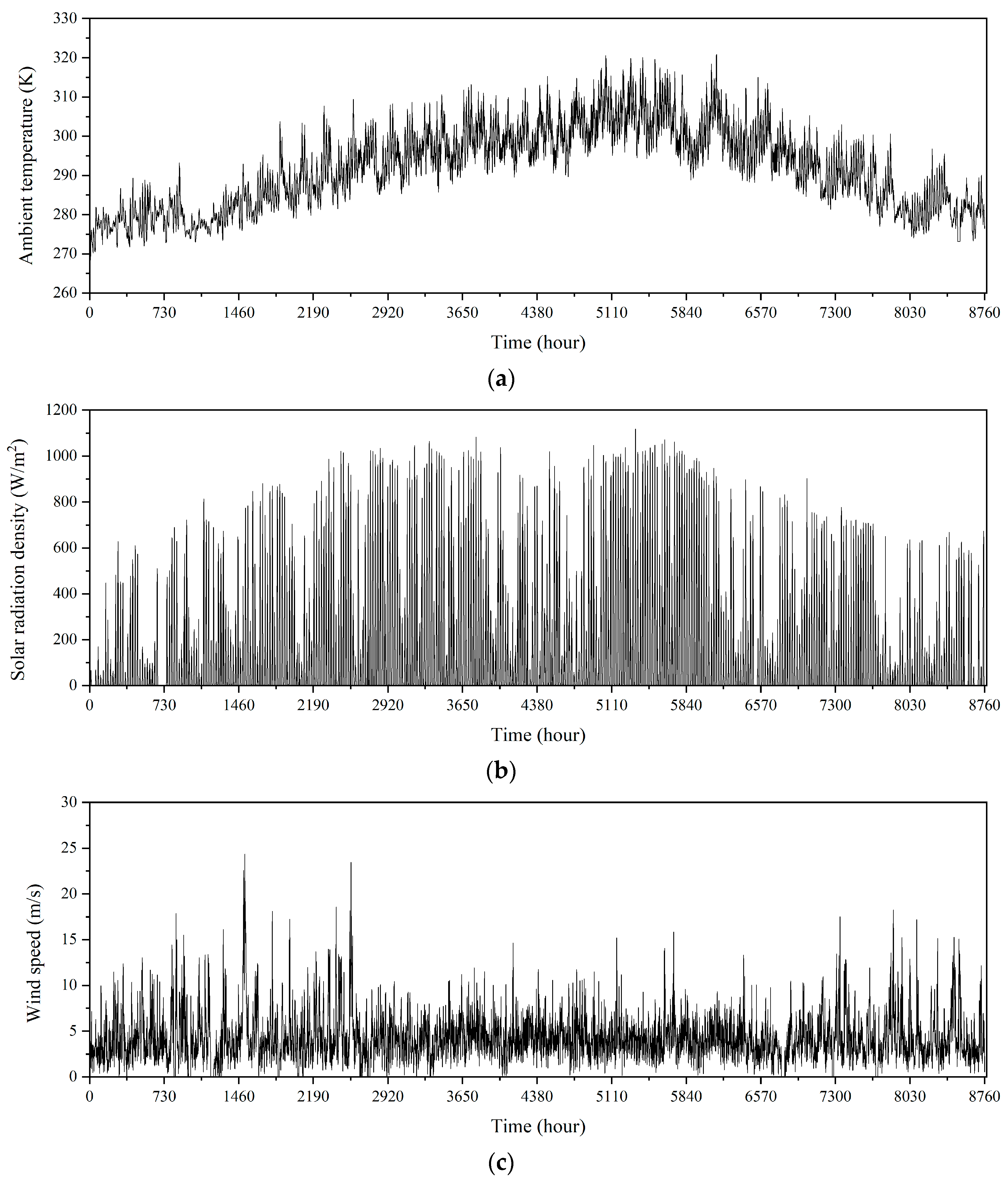
The PV output is determined by the solar radiation intensity, ambient temperature, and system’s physical installation parameters, as indicated in Formula (5). Moreover, the output is constrained by the installation capacity, as depicted by Formulas (7) and (8):

$$P_{PV}^t=P_{PV,0}\frac{G^t}{G_0}\left[1+k\left(T_s^t-T_{s,0}\right)\right],$$

(5)

$$T_s^t=T_a^t+0.03G^t,$$

(6)

$$0\le P_{PV}^t\le E_{PV},\mathrm{and}$$

(7)

$$0\le E_{PV}\le E_{PV}^{max},$$

(8)

where $P_{PV}^t$ is the PV output, $P_{PV,0}$ is the PV rated output, $G^t$ is the solar radiation intensity, $G_0$ is the solar radiation intensity under standard conditions, $k$ is the temperature coefficient, $T_s^t$ is the surface temperature of the PV, $T_{s,0}$ is the surface temperature of the PV under standard conditions, $T_a^t$ is the ambient temperature, $E_{PV}$ is the installation capacity, and $E_{PV}^{max}$ is the maximum installation capacity of the PV.

(2)

Wind turbine constraint

The output of a wind turbine, represented by Formula (9), is contingent upon the wind speed. Furthermore, the output is bounded by the installed capacity, as illustrated by Formulas (10) and (11):

$$P_{WT}^t=\left\{\begin{array}{c}0,v^t<v_{ci},v^t\ge v_{co}\\ \frac{v^t-v_{ci}}{v_N-v_{ci}}\cdot P_{WT,rated},v_{ci}\le v^t<v_N\\ P_{WT,rated},v_N\le v^t<v_{co}\end{array}\right.,$$

(9)

$$0\le P_{WT}^t\le E_{WT},\mathrm{and}$$

(10)

$$0\le E_{WT}\le E_{WT}^{max},$$

(11)

where $P_{WT}^t$ is the output of the wind turbine, $v^t$ is the wind speed, $v_{ci}$ is the cut in wind speed, $v_{co}$ is the cut out wind speed, $v_N$ is the rated wind speed, $P_{WT,rated}$ is the rated output of the wind turbine, $E_{WT}$ is the installation capacity of the wind turbine, and $E_{WT}^{max}$ is the maximum installation capacity of the wind turbine.

(3)

Gas turbine constraints

A gas turbine was employed to produce electricity and thermal energy through the consumption of natural gas. The electrical and thermal outputs are denoted by Formulas (12) and (13), respectively. Additionally, the output of the gas turbine was subject to limitations imposed by its installed capacity, as expressed by Formulas (14) and (15):

$$Q_{GT}^t=G_{hv}{V}_{GT,gas}^t{\eta }_{GT,q},$$

(12)

$$P_{GT}^t=G_{hv}{V}_{GT,gas}^t{\eta }_{GT,e},$$

(13)

$$0\le Q_{GT}^t\le E_{GT},\mathrm{and}$$

(14)

$$0\le E_{GT}\le E_{GT}^{max},$$

(15)

where $Q_{GT}^t$ is the thermal energy generated by the gas turbine, $G_{hv}$ is the calorific value of the natural gas, $V_{GT,gas}^t$ is the amount of natural gas consumed by the gas turbine, ${\eta }_{GT,q}$ is the thermal efficiency of the gas turbine, $P_{GT}^t$ is the electrical energy generated by the gas turbine, ${\eta }_{GT,e}$ is the electrical efficiency of the gas turbine, $E_{GT}$ is the installation capacity of the gas turbine, and $E_{GT}^{max}$ is the maximum installation capacity of the gas turbine.

(4)

Gas boiler constraints

Thermal energy can be produced by a gas boiler through the consumption of natural gas, as represented by Formula (16). Moreover, the thermal energy generated by a gas boiler is subject to limitations imposed by its installed capacity, as shown by Formulas (17) and (18):

$$Q_{GB}^t=G_{hv}{V}_{GB,gas}^t{\eta }_{GB},$$

(16)

$$0\le Q_{GB}^t\le E_{GB},\mathrm{and}$$

(17)

$$0\le E_{GB}\le E_{GB}^{max},$$

(18)

where $Q_{GB}^t$ is the thermal energy generated by the gas boiler, $V_{GB,gas}^t$ is the amount of natural gas consumed by the gas boiler, $E_{GB}$ is the installation capacity of the gas boiler, and $E_{GB}^{max}$ is the maximum installation capacity of the gas boiler.

(5)

Electric chiller constraints

An electric chiller employs electrical energy to produce cooling energy, as illustrated by Formula (19). The output of an electric chiller is constrained by its installed capacity, as indicated by Formulas (20) and (21):

$$Q_{EC}^t=P_{EC}^{t}CO{P}_{EC},$$

(19)

$$0\le Q_{EC}^t\le E_{EC},\mathrm{and}$$

(20)

$$0\le E_{EC}\le E_{EC,max},$$

(21)

where $Q_{EC}^t$ is the cooling energy generated by the electric chiller, $P_{EC}^t$ is the electrical energy consumed by the electric chiller, $CO{P}_{EC}$ is the electric chiller’s coefficient of performance, $E_{EC}$ is the installation capacity of the electric chiller, and $E_{EC,max}$ is the maximum installation capacity of the electric chiller.

(6)

Adsorption chiller

An adsorption chiller utilizes thermal energy absorption for the production of cooling energy, as denoted by Formula (22). The output of an adsorption chiller is constrained by its installed capacity, as represented by Formulas (23) and (24):

$$Q_{AC}^t=P_{AC}^t{\eta }_{AC},$$

(22)

$$0\le Q_{AC}^t\le E_{AC},\mathrm{and}$$

(23)

$$0\le E_{AC}\le E_{AC,max},$$

(24)

where $Q_{AC}^t$ is the cooling energy generated by the adsorption chiller, $P_{AC}^t$ is the thermal energy consumed by the adsorption chiller, ${\eta }_{AC}$ is the efficiency of the adsorption chiller, $E_{AC}$ is the installation capacity of the adsorption chiller, and $E_{AC,max}$ is the maximum installation capacity of the adsorption chiller.

(7)

Heat pump

A heat pump was employed for thermal energy generation through the consumption of electrical energy, as represented by Formula (25). The constraints on the heat pump’s output are detailed by Formulas (26) and (27):

$$Q_{HP}^t=P_{HP}^{t}CO{P}_{HP},$$

(25)

$$0\le Q_{HP}^t\le E_{HP},\mathrm{and}$$

(26)

$$0\le E_{HP}\le E_{HP}^{max},$$

(27)

where $Q_{HP}^t$ is the thermal energy generated by the heat pump, $P_{HP}^t$ is the electrical energy consumed by the heat pump, $CO{P}_{HP}$ is the heat pump’s coefficient of performance, $E_{HP}$ is the installation capacity of the heat pump, and $E_{HP}^{max}$ is the maximum installation capacity of the heat pump.

(8)

Electrical energy storage constraints

The constraints on the electrical energy storage encompassed the operation mode constraint and electric capacity constraints. The operation mode constraints for the electrical energy storage are articulated by Formula (28), signifying that the electrical energy storage system could operate in only one mode at a time, i.e., in charging, discharging, or idle mode, as follows:

$$v_{EES,ch}^t+v_{EES,dis}^t\le 1,$$

(28)

$$v_{EES,ch}^t\in \left\{0,1\right\},\mathrm{and}$$

(29)

$$v_{EES,dis}^t\in \left\{0,1\right\},$$

(30)

where $v_{EES,ch}^t$ and $v_{EES,dis}^t$ are the charging and discharging indicators of the electrical energy storage system, respectively.

The electrical capacity constraint specified that the charging and discharging capacities of the electrical energy storage system were limited by their respective maximum charging and discharging capacities, as expressed by Formulas (31) and (32):

$$0\le P_{EES,ch}^t\le P_{EES,ch,max} \mathrm{and}$$

(31)

$$0\le P_{EES,dis}^t\le P_{EES,dis,max},$$

(32)

where $P_{EES,ch}^t$ is the charging capacity of the electrical energy storage system, $P_{EES,dis}^t$ is the discharging capacity of the electrical energy storage system, $P_{ESS,ch,max}$ is the maximum charging capacity of the electrical energy storage system, and $P_{EES,dis,max}$ is the maximum discharging capacity of the electrical energy storage system.

Meanwhile, the charging and discharging capacities of the electrical energy storage were constrained by both its installation capacity and state of charge (SOC), as depicted below:

$$0\le E_{EES}\le E_{EES,max},$$

(33)

$$P_{EES,ch,max}\le {\sigma }_{EES}{E}_{EES},$$

(34)

$$P_{EES,dis,max}\le {\sigma }_{EES}{E}_{EES},$$

(35)

$$SO{C}_{EES}^{t+1}=SO{C}_{EES}^t+\frac{P_{EES,ch}^t{\eta }_{EES,ch}}{E_{EES}}-\frac{P_{EES,dis}^t{\eta }_{EES,dis}}{E_{EES}},\mathrm{and}$$

(36)

$$SO{C}_{EES}^{min}\le SO{C}_{EES}^t\le SO{C}_{EES}^{max},$$

(37)

where $E_{EES}$ is the installation capacity of the electrical energy storage system, $E_{EES,max}$ is the maximum installation capacity of the electrical energy storage system, ${\sigma }_{EES}$ is the capacity coefficient, $SO{C}_{EES}^t$ is the SOC of the electrical energy storage system, ${\eta }_{EES,ch}$ is the charging efficiency, ${\eta }_{EES,dis}$ is the discharging efficiency and $SO{C}_{EES}^{min}$ and $SO{C}_{EES}^{max}$ are the minimum and maximum values of the SOC, respectively.

(9)

Battery energy storage constraints

When employing a battery as the electrical energy storage system in an IES, irreversible capacity loss occurs due to diverse physical and chemical changes that are contingent on the battery’s lifecycle, environmental factors, and usage conditions [27]. The capacity loss of a battery encompasses calendar loss and cycle loss, as indicated by Formulas (38) and (39) [28]. Consequently, the energy storage capacity of a battery is constrained by both calendar and cycle loss as shown in Formula (40):

$$Q_{loss,cal}\left(\%\right)=k_{ref}\exp \left(-\frac{E_a}{R}\left(\frac{1}{T}-\frac{1}{T_{ref}}\right)\right)k_{SOC}\left(SOC\right)\sqrt{t},$$

(38)

$$Q_{loss,cyc}\left(\%\right)=k_{mean,SOC}{k}_{\mathsf{\Delta }SOC}{\left(EFC/100\right)}^n,\mathrm{and}$$

(39)

$$E_{EES}^{t+1}=E_{EES}^t-E_{EES}^t{Q}_{loss,cal}-E_{EES}^t{Q}_{loss,cyc},$$

(40)

where $Q_{loss,cal}$ is the calendar capacity loss, $k_{ref}$ is the influence coefficient under the reference temperature and SOC, $E_a$ is the activation energy, $R$ is the gas constant, $T$ is the temperature, $T_{ref}$ is the reference temperature, $k_{SOC}\left(SOC\right)$ is the coefficient regarding the SOC, $\sqrt{t}$ is the influence coefficient regarding the time, $Q_{loss,cyc}$ is the cycle capacity loss, $k_{mean,SOC}$ the coefficient regarding the mean SOC, $k_{\Delta SOC}$ is the coefficient regarding the $\Delta SOC$, $EFC$ is equivalent to full cycles, and $n$ is a coefficient.

(10)

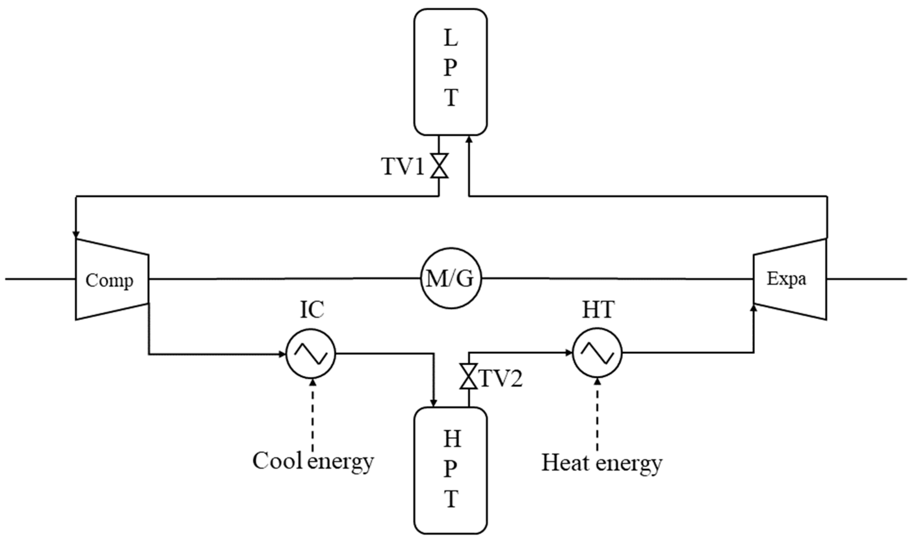
Compressed CO₂ energy storage system constraints

When utilizing a CCES system as an electrical energy storage system in an IES, the charging and discharging capacities of the CCES system are additionally constrained by its SOC, which was provided for in our previous study and is expressed by Formulas (41) to (44) [25]:

$$\begin{array}{c}\frac{v_{EES,ch}^t\cdot {\dot{m}}_{W_{Comp}}^t\cdot t_{st}}{M_{total}}\le SO{C}_{max}^{W_{Comp}}\end{array}-SO{C}^t,$$

(41)

$$SO{C}_{max}^{W_{Comp}}=\frac{{\dot{m}}_{W_{Comp}}^t\cdot t_{c,W_{Comp}}}{M_{total}},$$

(42)

$$\begin{array}{c}\frac{v_{EES,dis}^t\cdot {\dot{m}}_{W_{Expa}}^t\cdot t_{st}}{M_{total}}\le \end{array}SO{C}^t-SO{C}_{min}^{W_{Expa}},\mathrm{and}$$

(43)

$$SO{C}_{min}^{W_{Expa}}=\frac{M_{total}-{\dot{m}}_{W_{Expa}}\cdot t_{d,W_{Expa}}}{M_{total}},$$

(44)

where ${\dot{m}}_{W_{Comp}}^t$ is the mass flow rate of the compressor, $t_{st}$ is the duration of a single time interval at which the compressor and the expander operate, $M_{total}$ is the total mass of the CO₂ in the high-pressure gas tank, $SO{C}_{max}^{W_{Comp}}$ is the maximum SOC of the CCES system at a certain compressor’s electric capacity ($W_{Comp}$), $t_{c,W_{Comp}}$ is the duration of the charging process if the CCES system charges at the constant electric capacity $W_{Comp}$, ${\dot{m}}_{W_{Expa}}^t$ is the mass flow rate of the expander, $SO{C}_{min}^{W_{Expa}}$ is the minimum SOC of the CCES system at a certain expander’s electric capacity, and $t_{d,W_{Expa}}$ is the duration of the discharging process if the CCES system discharges at the constant electric capacity $W_{Expa}$.

The definition of the SOC for the CCES system is presented by Formula (45), and the SOC must adhere to the constraint outlined in Formula (46):

$$SO{C}^t=\frac{M^t}{M_{total}} \mathrm{and}$$

(45)

$$\begin{array}{c}SO{C}^{t+1}=SO{C}^t+v_{EES,ch}^t\frac{{\dot{m}}_{W_{Comp}}^t\cdot t_{st}}{M_{total}}-v_{EES,dis}^t\frac{{\dot{m}}_{W_{Expa}}^t\cdot t_{st}}{M_{total}}\end{array},$$

(46)

where $M^t$ is the stored mass of the CO₂ at the time $t$ in the high-pressure gas tank.

(11)

Thermal and cooling energy storage constraints

The constraints on the thermal and cooling energy storage system were analogous to those of the electrical energy storage system, encompassing mode restrictions and charging and discharging capacity constraints, as illustrated below:

$$v_{j,ch}^t+v_{j,dis}^t\le 1,$$

(47)

$$v_{j,ch}^t\in \left\{0,1\right\},$$

(48)

$$v_{j,dis}^t\in \left\{0,1\right\},$$

(49)

$$0\le P_{j,ch}^t\le P_{j,ch,max},$$

(50)

$$0\le P_{j,dis}^t\le P_{j,dis,max},$$

(51)

$$0\le E_j\le E_{j,max},$$

(52)

$$P_{j,ch,max}\le {\sigma }_j{E}_j,$$

(53)

$$P_{j,dis,max}\le {\sigma }_j{E}_j,\mathrm{and}$$

(54)

$$SO{C}_j^{t+1}=SO{C}_j^t+\frac{P_{j,ch}^t{\eta }_{j,ch}}{E_j}-\frac{P_{j,dis}^t{\eta }_{j,dis}}{E_j},$$

(55)

where the subscript $j$ denotes the thermal energy storage and cooling energy storage.

(12)

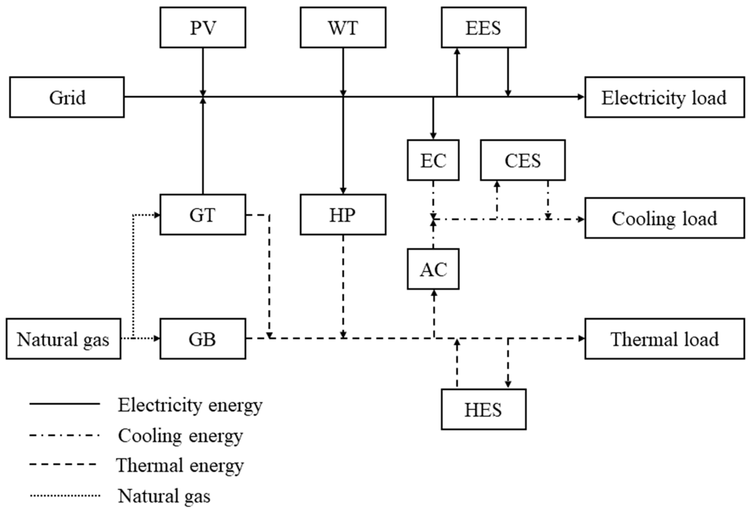
Energy balance constraints

The energy balance constraints comprised the electrical energy balance, thermal energy balance, and cooling energy balance, as depicted below:

$$P_{PV}^t+P_{WT}^t+P_{GT}^t+P_{grid}^t+P_{EES,dis}^t-P_{EES,ch}^t-P_{EC}^t-P_{HP}^t=P_{e,load}^t,$$

(56)

$$Q_{EC}^t+Q_{AC}^t+P_{CES,dis}^t-P_{CES,ch}^t=P_{c,load}^t,\mathrm{and}$$

(57)

$$Q_{GT}^t+Q_{GB}^t+Q_{HP}^t+P_{HES,dis}^t-P_{AC}^t-P_{HES,ch}^t=P_{h,load}^t,$$

(58)

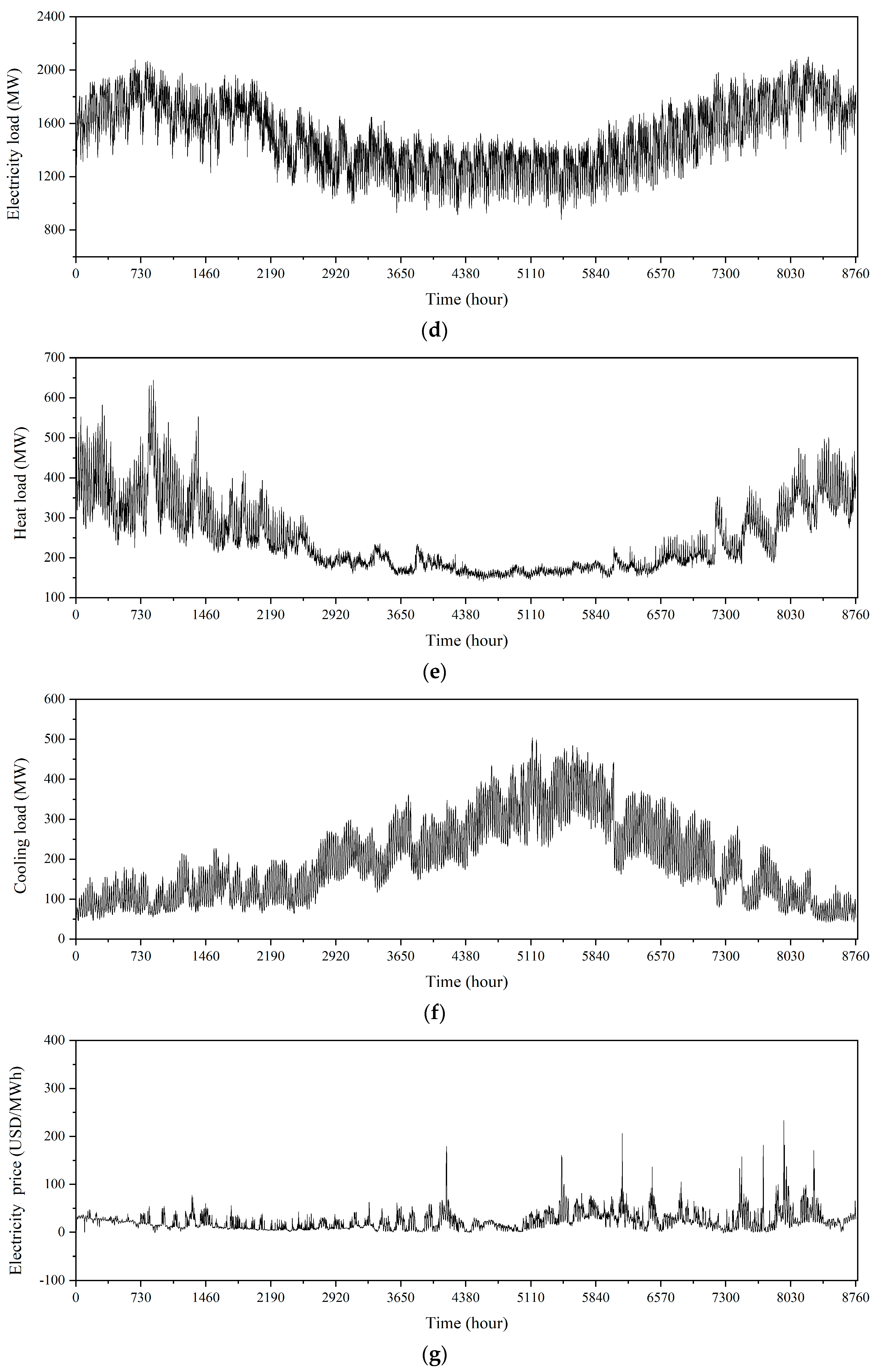
where $P_{e,load}^t$ is the electricity load, $P_{c,load}^t$ is the cooling load, and $P_{h,load}^t$ is the heat load.

2.3. Solving Method

The optimization problem was expressed as a mixed inter linear programming (MILP) problem, which was solved by Gurobi in MATLAB with version 2018a. The optimization processes are summarized in

Table 1. The process for optimizing the configuration and operation of the IES.

Step	Optimization Process
Step 1.	Input weather, load, and electricity price data.
Step 2.	Optimize the configuration of the IES by solving Formula (1) subjected to Formulas (5)–(58) using the Gurobi optimizer.
Step 3.	Develop the calendar and cycle loss model of the BES system.
Step 4.	Configure the IES–BES system based on the capacities determined in Step 2 and the loss model established in Step 3, followed by optimizing its operation using the Gurobi optimizer.
Step 5.	Determine the key parameters of the CCES system based on the capacity from Step 2.
Step 6.	Calculate the SOC and electrical capacity boundaries based on the following developed dynamic model: $W_{Comp,min}$, $W_{Comp,max}$, $W_{Expa,min}$, $W_{Expa,max}$, $SO{C}_{min}$, and $SO{C}_{max}$.
Step 7.	Calculate the maximum and minimum values of the CCES system at different compressor and expander electrical capacities based on the definitions in Formulas (42) and (44) and the following developed model: $SO{C}_{max}^{W_{Comp}}$ and $SO{C}_{min}^{W_{Expa}}$.
Step 8.	Configure the IES–CCES system utilizing the capacities determined in Step 2 and the parameters established in Steps 5–7, followed by optimizing its operation with the Gurobi optimizer.

.

3. Case Study

To assess the techno-economic performance of integrating a CCES in an IES, this section introduces the case study, encompassing the data set, model-setting parameters, and CCES system.

3.1. Data Set

The dataset comprises the ambient temperature, solar radiation density, wind speed, electricity load, cooling load, heat load, and electricity prices from the Nordic electricity market in 2022, as depicted in Figure 2 [29]. These data were employed for optimizing the configuration and operation of the IES system.

3.2. Model Setting

The main parameters and unit investment cost of each piece of equipment are summarized in

Table 2. Main parameters of each piece of equipment in the model.

Parameter	Value
Solar radiation intensity under standard conditions (W/m2)	1
Surface temperature of the PV under standard conditions (K)	298
Cut in the wind speed (m/s)	3
Cut out of the wind speed (m/s)	25
Rated wind speed (m/s)	12
Calorific value of the natural gas (kWh/m3)	9.7
Thermal efficiency of the gas turbine (%)	0.54
Electrical efficiency of the gas turbine (%)	0.34
Efficiency of the gas boiler (%)	0.89
Coefficient of performance of the electric chiller	3.45
Coefficient of performance of the heat pump	3.45
Efficiency of the adsorption chiller (%)	0.79
Charging efficiency of the energy storage system (%)	0.95
Discharging efficiency of the energy storage system (%)	0.95
Capacity coefficient of the energy storage system	0.5

and

Table 3. The unit investment cost and lifetime of each piece of equipment in the model.

Component	Unit Investment Cost (USD/kW)	Lifetime	O&M Coefficient (%)
Photovoltaic panels	705	30	1
Wind turbine	1233	30	2
Gas turbine	928	30	2
Gas boiler	200	30	0.5
Electric chiller	157	30	2
Adsorption chiller	185	30	1
Electrical energy storage	100	15	2.5
Thermal energy storage	14	30	2
Cooling energy storage	14	30	2

[30,31,32].

The calendar and cycle capacity losses of the battery energy storage system, derived from the experimental data, are presented as follows [28]:

$$Q_{loss,cal}\left(\%\right)=0.0013\cdot e^{2059.9\cdot (\frac{1}{T}-\frac{1}{298.15})}\cdot (2.86\cdot {(SOC-0.5)}^{0.3}+0.6)\cdot \sqrt{t} \mathrm{and}$$

(59)

$$Q_{loss,cyc}\left(\%\right)=3.25\cdot SO{C}_{mean}\cdot (1+3.25\cdot \Delta SOC-2.25\cdot \Delta SO{C}^2)\cdot {(\frac{EFC}{100})}^{0.453},$$

(60)

where $SO{C}_{mean}$ is the mean SOC.

3.3. Compressed CO₂ Energy Storage System

A schematic diagram of the CCES system used in the IES system is shown in Figure 3 [23], and it consisted of a low-pressure gas tank (LPT), a high-pressure gas tank (HPT), a compressor (Comp), an expander (Expa), throttling valves (TVs), an intercooler (IC), and a heater (HT).

The main parameters of the CCES system are summarized in

Table 4. Main parameters of the CCES system.

Parameter	Value
Rated isentropic efficiency of the compressor (%)	89
Rated isentropic efficiency of the expander (%)	88
The initial pressure of the low-pressure gas tank (MPa)	1.0
The initial pressure of the high-pressure gas tank (MPa)	2.3
The initial temperature of the gas tank (K)	300
The inlet temperature of the expander (K)	600
The pressure ratio range of the compressor	7.8–14.0
The pressure ratio range of the expander	4.5–10.1

[25,33].

An economic model of the CCES system is summarized as

Table 5. An economic model of the CCES system.

Component	Economic Model *
Compressor	$C_{Comp}=71.1{\dot{m}}_{Comp}\frac{1}{0.92-{\eta }_{Comp}}\frac{P_{out}}{P_{in}}\ln (\frac{P_{out}}{P_{in}})$
Expander	$C_{Expa}=4405{(\frac{W_{Expa}}{1000})}^{0.7}$
Gas tank	$C_{Tank}=4042V_{Tank}^{0.506}$
Total	$C_{CCES}=C_{Comp}+C_{Expa}+C_{Tank}$

* In Table 5, $P$ denotes the pressure, $\eta$ is the efficiency, and $C$ denotes the investment cost.

[18].

4. Result and Discussion

This section presents and analyzes the optimization results, comprising three components: the configuration results, the operation results, and the cycle results. The configuration results section discusses the installation capacities and investment costs of both the IES–CCES and IES–BES systems. The operation results section delves into the detailed operation and operational costs of the IES–CCES and IES–BES systems, specifically, where the capacity loss of the BES system is not considered. The cycle results section addresses the total costs throughout the systems’ lifespans for both the IES–CCES and IES–BES systems, considering the capacity loss of the BES system.

4.1. Configuration Result

The optimization results are summarized in

Table 6. The installation capacities and investment costs of each piece of equipment.

Equipment	PV	WT	GT	GB	EC	AC	HP	EES	CES	HES
Capacity (MW)	500	500	996	0	230	267	0	267	300	350
Investment cost (MUSD)	28.2	49.3	73.9	0	2.9	4.0	0	/	0.3	0.4

, including the installation capacities and investment costs for each piece of equipment.

Table 6 indicates that the installation capacities of the gas boiler and heat pump were zero due to their high investment costs. Additionally, the maximum heat load was 644 MW, as shown in Figure 2e, and the maximum thermal energy outputs of the gas turbine and heat energy storage were 535.1 MW and 175 MW, respectively. Consequently, the combined output of the gas turbine and heat energy storage was sufficient for meeting the heat load, eliminating the need for additional heat-generating equipment and reducing the overall investment cost of the IES.

Table 6 reveals the installation capacity of 267 MWh for the electrical energy storage system. Subsequently, the key parameters of the CCES and BES systems could be derived, as outlined in

Table 7. Main parameters of the CCES and BES system.

Parameters	CCE	BES
The volume of the high-pressure gas tank (m3)	76,000	/
The volume of the low-pressure gas tank (m3)	3,600,000	/
Charging capacity range (MW)	57–110	0–133.5
Discharging capacity range (MW)	30–120	0–133.5
Round-trip efficiency (%)	56.7	90.3
Investment cost (MUSD)	2.9	2.4

.

Table 7 indicates that the charging capacity range of the CCES system spanned from 57 MW to 110 MW, while its discharging capacity ranged from 30 MW to 120 MW. A comparison with the BES system revealed that the capacity range of the CCES system was narrower than that of the BES system, which was 0 MW to 133.5 MW. This limitation was attributed to the pressure ratio limitations of the compressor and the expander, which set a lower bound on the electrical capacity of both components. Additionally, the higher charging and discharging efficiencies of the BES system resulted in a round-trip efficiency (RTE) of 90.3%, whereas the CCES system attained an RTE of 56.7% due to the lower efficiency of the compressor and expander, along with an additional thermal energy input.

Derived from the unit investment costs of the individual components, the investment cost of the IES–CCES system amounted to MUSD 161.9. This figure was marginally higher (MUSD 0.5) compared to the investment cost of the IES–BES, which totaled MUSD 161.4. The increased cost was attributed to the higher investment cost associated with the CCES system.

4.2. Operation Result

The operational details of the IES–CCES system were exemplified by using a randomly chosen day, specifically, 5 January 2022. In this context, Figure 4a delineates the electrical energy balance, Figure 4b portrays the thermal energy balance, Figure 4c illustrates the cooling energy balance, and Figure 4d depicts the electricity prices on 5 January 2022.

As depicted in Figure 4, the CCES system strategically charged during periods of lower load and electricity prices, subsequently discharging during higher load and electricity price periods to minimize the operational cost of the IES–CCES system. Figure 4a shows that a substantial portion of the electrical energy supply, amounting to 32.2 GW and constituting 80.3% of the total electricity energy supply, was procured from the grid. Further, Figure 4b,c reveals that the adsorption chiller remained inactive as the cooling energy requirements were adequately met through the collaboration between the electric chiller and the cooling energy storage system.

The daily total operational cost of the IES–CCES system, illustrated in Figure 5, was computed by aggregating the costs associated with the purchasing electricity, acquiring natural gas, and the CO₂ emissions. Notably, the daily operational cost exhibited a pattern mirroring the load fluctuations. Upon cumulating the daily operational costs, the annual operational cost of the IES–CCES system amounted to MUSD 766.6.

In the absence of considering the capacity loss of the BES system, the detailed operation of the IES–BES system on 5 January 2022, as shown in Figure 6, was employed for a comparison with the operation of the IES–CCES system.

As depicted in Figure 6, the operations of the IES–CCES and IES–BES systems exhibited similarities. However, the detailed operations of the CCES and BES systems differed. As shown by the red dotted circle in Figure 4a, the CCES system charged during the second and third schedule times and discharged from the seventeenth to twentieth schedule times. In contrast, the BES system discharged during the eighteenth and nineteenth schedule times, as shown by the red dotted circle in Figure 6a, with a discharge period that was two hours shorter than that of the CCES system. This difference arose because additional thermal energy needed to be input into the CCES system when it was in the discharge mode, as indicated by the black solid circle in Figure 4b. This necessitated extra natural gas purchasing and CO₂ emissions. Consequently, the CCES system operated for an additional hour to reduce the electricity purchases from the grid and mitigate the costs associated with the extra natural gas purchase and CO₂ emissions.

In comparison to the daily operational cost of the IES–BES system depicted in Figure 7, it was evident that the daily operational cost of the IES–CCES system was higher. This discrepancy arose due to the additional consumption of natural gas and CO₂ emissions. Using 5 January 2022 as an illustration, the extra thermal energy input into the CCES system amounted to 120 MWh, resulting in the IES–CCES system consuming an additional 1.8 million m³ of natural gas. Over the entire year 2022, the CCES system required an extra thermal energy input of 22.4 GWh, leading to the IES–CCES system consuming 3.5 million m³ more natural gas than the IES–BES system, which consumed a total of 486.3 million m³ of natural gas. Consequently, the annual operational cost of the IES–CCES system was MUSD 0.5 higher than that of the IES–BES system, amounting to MUSD 766.1.

4.3. Cycle Result

During the entire operational lifespan, the capacity of the BES system underwent deterioration attributed to calendar and cycle loss. Figure 8 illustrates the capacity and cumulative equivalent cycles of the BES system over its 15-year lifespan.

As depicted in Figure 8, the BES system experienced an average of 138 equivalent cycles per year to meet the load requirements of the IES–BES system, resulting in energy capacity loss. Over 15 years of operation, the energy storage capacity of the BES system diminished to 56 MWh, constituting only 21.0% of its initial energy capacity. This reduction in energy capacity contributed to an elevated annual operation cost for the IES–BES system, as illustrated in Figure 9.

As indicated in Figure 9, the annual operation cost of the IES–CCES system remained constant over the 15-year period due to the consistent energy storage capacity of the CCES system. In contrast, the diminished energy capacity of the BES system resulted in an increased consumption of natural gas, rising from 486.3 million m³ to 486.8 million m³. Consequently, the annual operation cost of the IES–BES system escalated from MUSD 766.17 to USD 767.31. Notably, a crossover point was observed in the sixth year, indicating that the annual operation cost of the IES–BES system surpassed that of the IES–CCES system beyond the sixth year.

Nevertheless, as the energy capacity of the BES system diminished to a specific threshold, its removal became necessary, requiring the incorporation of a new BES system into the IES system. Consequently, a parameter defined as the energy capacity coefficient (ECC (%)), denoting the ratio of residual energy capacity to the initial capacity, was introduced to assess the impacts of the varied decommissioning capacities of the BES system on the total cost throughout the system’s 30-year lifespan for an IES system, as depicted in Figure 10.

As illustrated in Figure 10, the total cost of the IES–BES system initially experienced a decline, followed by an ascent with the increasing ECC. At an ECC of 30%, the BES system operated for 12 years before being replaced. Consequently, its operational cost decreased compared to the scenario where it operated continuously for 15 years, resulting in the minimum total cost. However, with the higher ECC values, although the operational costs decreased, the frequency of incorporating a new BES system into the IES system rose. Hence, the total cost of the IES–BES system increased when the ECC exceeded 30%. Conversely, a significant upswing in the total cost occurred when the ECC reached 80%, which was attributed to a total of 10 instances of incorporating a new BES system into the IES system, incurring elevated investment costs.

Over a continuous 30-year operational period for the IES–CCES system, the total cost amounted to only MUSD 23,159.9, indicating a reduction of MUSD 4.4 compared to the minimum total cost of the IES–BES system.

5. Conclusions

This paper proposed the integration of a compressed CO₂ energy storage system (CCES) with an integrated energy system (IES–CCES), which could address the capacity loss in a battery energy storage (BES) system and provide benefits for configuring a large-scale integrated energy system (IES). The proposed system was further compared with an IES with a BES system (IES–BES). The following conclusions were obtained:

(1)

With an energy storage capacity of 267 MWh, the BES system exhibited a higher round-trip efficiency (RTE) of 90.3%, surpassing the CCES system’s RTE of 56.7%. Simultaneously, the total investment cost of the IES–CCES system amounted to MUSD 161.9, representing a slight increase, MUSD 0.5, compared to the IES–BES system.

(2)

When the capacity loss of the BES system was not considered, the annual operation cost of the IES–CCES system was MUSD 766.6, representing an increase of MUSD 0.5 compared to that of the IES–BES system.

(3)

When the capacity loss of the BES system was considered, the annual operation cost of the IES–CCES was lower than the annual operation cost of the IES–BES system beyond the sixth year. Over a 35-year lifespan for an IES system, the total cost of the IES–CCES system was MUSD 23159.9, which was MUSD 4.4 lower than the minimum total cost of the IES–BES system when the BES system was removed at a threshold of 30%.

References

1. Song, C.; Liu, Q.; Ji, N.; Deng, S.; Zhao, J.; Li, Y.; Song, Y.; Li, H. Alternative pathways for efficient CO2 capture by hybrid processes—A review. Renew. Sustain. Energy Rev. 2018, 82, 215–231. [Google Scholar] [CrossRef]
2. Hansen, K.; Breyer, C.; Lund, H. Status and perspectives on 100% renewable energy systems. Energy 2019, 175, 471–480. [Google Scholar] [CrossRef]
3. He, W.; King, M.; Luo, X.; Dooner, M.; Li, D.; Wang, J. Technologies and economics of electric energy storages in power systems: Review and perspective. Adv. Appl. Energy 2021, 4, 100060. [Google Scholar] [CrossRef]
4. Song, D.; Meng, W.; Dong, M.; Yang, J.; Wang, J.; Chen, X.; Huang, L. A critical survey of integrated energy system: Summaries, methodologies and analysis. Energy Convers. Manag. 2022, 266, 115863. [Google Scholar] [CrossRef]
5. Zhang, W.; Lou, J.; Wang, C.; Yu, Q.; Wang, J.; Chang, X.; Liang, Y. Review and prospect of modeling and optimization of integrated energy system. In Proceedings of the 2020 IEEE 3rd Student Conference on Electrical Machines and Systems (SCEMS), Jinan, China, 4–6 December 2020. [Google Scholar]
6. Wang, Y.; Song, F.; Ma, Y.; Zhang, Y.; Yang, J.; Liu, Y.; Zhang, F.; Zhu, J. Research on capacity planning and optimization of regional integrated energy system based on hybrid energy storage system. Appl. Therm. Eng. 2020, 180, 115834. [Google Scholar] [CrossRef]
7. Wang, M.; Yu, H.; Jing, R.; Liu, H.; Chen, P.; Li, C. Combined multi-objective optimization and robustness analysis framework for building integrated energy system under uncertainty. Energy Convers. Manag. 2020, 208, 112589. [Google Scholar] [CrossRef]
8. Fu, Y.; Lin, H.; Feng, B.; Ma, C.; Sun, Q.; Wennersten, R. Off-design characteristics of energy conversion equipment in integrated energy systems. J. Clean. Prod. 2023, 407, 136941. [Google Scholar] [CrossRef]
9. Pan, C.; Fan, H.; Zhang, R.; Sun, J.; Wang, Y.; Sun, Y. An improved multi-timescale coordinated control strategy for an integrated energy system with a hybrid energy storage system. Appl. Energy 2023, 343, 121137. [Google Scholar] [CrossRef]
10. Liu, S.; Zhou, C.; Guo, H.; Shi, Q.; Song, T.E.; Schomer, I.; Liu, Y. Operational optimization of a building-level integrated energy system considering additional potential benefits of energy storage. Prot. Control Mod. Power Syst. 2021, 6, 4. [Google Scholar] [CrossRef]
11. Han, X.; Ji, T.; Zhao, Z.; Zhang, H. Economic evaluation of batteries planning in energy storage power stations for load shifting. Renew. Energy 2015, 78, 643–647. [Google Scholar] [CrossRef]
12. Chen, Y.; Xu, J.; Wang, J.; Lund, P.D.; Wang, D. Configuration optimization and selection of a photovoltaic-gas integrated energy system considering renewable energy penetration in power grid. Energy Convers. Manag. 2022, 254, 115260. [Google Scholar] [CrossRef]
13. Liu, Z.; Cui, Y.; Wang, J.; Yue, C.; Agbodjan, Y.S.; Yang, Y. Multi-objective optimization of multi-energy complementary integrated energy systems considering load prediction and renewable energy production uncertainties. Energy 2022, 254, 124399. [Google Scholar] [CrossRef]
14. Wang, Y.; Liu, Z.; Cai, C.; Xue, L.; Ma, Y.; Shen, H.; Chen, X.; Liu, L. Research on the optimization method of integrated energy system operation with multi-subject game. Energy 2022, 245, 123305. [Google Scholar] [CrossRef]
15. Guo, J.; Wu, D.; Wang, Y.; Wang, L.; Guo, H. Co-optimization method research and comprehensive benefits analysis of regional integrated energy system. Appl. Energy 2023, 340, 121034. [Google Scholar] [CrossRef]
16. Pan, C.; Jin, T.; Li, N.; Wang, G.; Hou, X.; Gu, Y. Multi-objective and two-stage optimization study of integrated energy systems considering P2G and integrated demand responses. Energy 2023, 270, 126846. [Google Scholar] [CrossRef]
17. Lu, M.; Du, Y.; Yang, C.; Zhang, Z.; Wang, H.; Sun, S. Performance analysis and multi-objective optimization of a combined system of Brayton cycle and compression energy storage based on supercritical carbon dioxide. Appl. Therm. Eng. 2024, 236, 121837. [Google Scholar] [CrossRef]
18. Yang, X.; Liu, Z.; Jia, W.; Li, H.; Yang, X. Justification of CO2 as the working fluid for a compressed gas energy storage system: A thermodynamic and economic study. J. Energy Storage 2020, 27, 101132. [Google Scholar]
19. Huang, Q.; Yao, J.; Hu, Y.; Liu, S.; Li, H.; Sun, Q. Integrating compressed CO2 energy storage in an oxy-coal combustion power plant with CO2 capture. Energy 2022, 254, 124493. [Google Scholar] [CrossRef]
20. Gao, C. Performance investigation of solar-assisted supercritical compressed carbon dioxide energy storage systems. J. Energy Storage 2024, 79, 110179. [Google Scholar] [CrossRef]
21. Zhao, R.; Liu, Z. Thermo-economic performance of a compressed CO2 energy storage system with a flexible gas holder. J. Energy Storage 2023, 60, 106675. [Google Scholar] [CrossRef]
22. Zhang, Y.; Liang, T.; Yang, K. An integrated energy storage system consisting of Compressed Carbon dioxide energy storage and Organic Rankine Cycle: Exergoeconomic evaluation and multi-objective optimization. Energy 2022, 247, 123566. [Google Scholar] [CrossRef]
23. Huang, Q.; Feng, B.; Liu, S.; Ma, C.; Li, H.; Sun, Q. Dynamic operating characteristics of a compressed CO2 energy storage system. Appl. Energy 2023, 341, 120985. [Google Scholar] [CrossRef]
24. Zhang, Y.; Wu, Y.; Yang, K. Dynamic characteristics of a two-stage compression and two-stage expansion Compressed Carbon dioxide energy storage system under sliding pressure operation. Energy Convers. Manag. 2022, 254, 115218. [Google Scholar] [CrossRef]
25. Zhang, B.; Yang, J.; Tian, S.; Huang, Q.; Wang, W.; Sun, Q.; Ren, X. Techno-Economic Evaluation of a Compressed CO2 Energy Storage System for Load Shifting Based on Dynamic Modelling. Energies 2023, 16, 7894. [Google Scholar] [CrossRef]
26. Hao, J.; Zheng, P.; Li, Y.; Zhang, Z.; Zhang, J.; Yang, J.; Yue, Y.; Li, X. Study on the operational feasibility domain of combined heat and power generation system based on compressed carbon dioxide energy storage. Energy 2023, 291, 130122. [Google Scholar] [CrossRef]
27. Zhao, T.; Li, W.; Traversy, M.; Choi, Y.; Ghahreman, A.; Zhao, Z.; Zhang, C.; Zhao, W.; Song, Y. A review on the recycling of spent lithium iron phosphate batteries. J. Environ. Manag. 2024, 351, 119670. [Google Scholar] [CrossRef] [PubMed]
28. Saxena, S.; Hendricks, C.; Pecht, M. Cycle life testing and modeling of graphite/LiCoO2 cells under different state of charge ranges. J. Power Sources 2016, 327, 394–400. [Google Scholar] [CrossRef]
29. EMBER. European Power Price Tracker. Available online: https://ember-climate.org/ (accessed on 6 January 2023).
30. Wang, Y.; Wang, Y.; Huang, Y.; Li, F.; Zeng, M.; Li, J.; Wang, X.; Zhang, F. Planning and operation method of the regional integrated energy system considering economy and environment. Energy 2019, 171, 731–750. [Google Scholar] [CrossRef]
31. Qiao, Y.; Hu, F.; Xiong, W.; Guo, Z.; Zhou, X.; Li, Y. Multi-objective optimization of integrated energy system considering installation configuration. Energy 2023, 263, 125785. [Google Scholar] [CrossRef]
32. Li, J.; Xu, W.; Cui, P.; Qiao, B.; Feng, X.; Xue, H.; Wang, X.; Xiao, L. Optimization configuration of regional integrated energy system based on standard module. Energy Build. 2020, 229, 110485. [Google Scholar] [CrossRef]
33. Zhao, P.; Gao, L.; Wang, J.; Dai, Y. Energy efficiency analysis and off-design analysis of two different discharge modes for compressed air energy storage system using axial turbines. Renew. Energy 2016, 85, 1164–1177. [Google Scholar] [CrossRef]
Figure 1. A schematic diagram of an integrated energy system.
Energies 17 01570 g001
Figure 2. The ambient temperature, solar radiation density, wind speed, electricity load, heat load, cooling load, and electricity price in 2022: (a) the ambient temperature in 2022; (b) the solar radiation density in 2022; (c) the wind speed in 2022; (d) the electricity load in 2022; (e) the heat load in 2022; (f) the cooling load in 2022; and (g) the electricity price in 2022.
Energies 17 01570 g002aEnergies 17 01570 g002b
Figure 3. A schematic diagram of the compressed CO2 energy storage system.
Energies 17 01570 g003
Figure 4. (a) The electrical energy balance of the IES–CCES system on 5 January 2022; (b) the thermal energy balance of the IES–CCES system on 5 January 2022; (c) the cooling energy balance of the IES–CCES system on 5 January 2022; and (d) the electricity price on 5 January 2022.
Energies 17 01570 g004aEnergies 17 01570 g004b
Figure 5. The daily operation cost of the IES–CCES system.
Energies 17 01570 g005
Figure 6. (a) The electrical energy balance of the IES–BES system on 5 January 2022; (b) the thermal energy balance of the IES–BES system on 5 January 2022; and (c) the cooling energy balance of the IES–BES system on 5 January 2022.
Energies 17 01570 g006
Figure 7. The daily operation cost of the IES–BES system.
Energies 17 01570 g007
Figure 8. The capacity and accumulative equivalent cycles of the battery energy storage system.
Energies 17 01570 g008
Figure 9. The annual operation costs of the IES–CCES and IES–BES systems.
Energies 17 01570 g009
Figure 10. Effects of the ECC on the total cost of the IES–BES system.
Energies 17 01570 g010