Article

A Non-Iterative Coordinated Scheduling Method for a AC-DC Hybrid Distribution Network Based on a Projection of the Feasible Region of Tie Line Transmission Power

1
School of Electrical Engineering, Guangxi University, Nanning 530004, China
2
Zigong Power Supply Bureau, Sichuan Power Grid Co., Ltd., Zigong 643031, China
*
Author to whom correspondence should be addressed.
Energies 2024, 17(6), 1462; https://doi.org/10.3390/en17061462
Submission received: 7 February 2024 / Revised: 14 March 2024 / Accepted: 15 March 2024 / Published: 18 March 2024
(This article belongs to the Section F3: Power Electronics)

Abstract

:
AC-DC hybrid distribution grids realize power transmission through tie lines. Accurately characterizing the power exchange capacity between regional grids while ensuring safe grid operation is the basis for the coordinated scheduling of resources in interconnected distribution grids. However, most of the current AC/DC hybrid models are linear, and it is challenging to ensure the accuracy criteria of the obtained feasible regions. In this paper, a two-stage multi-segment boundary approximation method is proposed to characterize the feasible region of hybrid distribution grid tie line operation. Information such as security operation constraints are mapped to the feasible region of the boundary tie line to accurately characterize the transmission exchange capacity of the tie line. To avoid the limitations of linear models, the method uses a nonlinear model to iteratively search for boundary points of the feasible region. This ensures high accuracy in approximating the real feasible region shape and capacity limitations. A convolutional neural network (CNN) is then utilized to map the given boundary and cost information to obtain an estimated equivalent operating cost function for the contact line, overcoming the inability of previous methods to capture nonlinear cost relationships. This provides the necessary cost information in a data-driven manner for the economic dispatch of hybrid AC-DC distribution networks. Numerical tests demonstrate the effectiveness of the method in improving coordination accuracy while preserving regional grid privacy. The key innovations are nonlinear modeling of the feasible domain of the contact line and nonlinear cost fitting for high-accuracy dispatch.

1. Introduction

As power electronics technology advances, building an AC/DC hybrid distribution network has gained popularity [1]. The direct current (DC) distribution network provides several benefits over an AC distribution network, such as strong system stability, reduced transmission loss, variable control modes, and a large power supply capacity [2]. At present, when the traditional AC distribution network evolves into an AC/DC hybrid distribution network [3,4], the most important problem to be solved is how to schedule the hybrid distribution network to achieve the optimal operation of the distribution network [5].
The unified centralized optimization method establishes a detailed model of each regional power grid, which can realize the optimal operation of a multi-regional power system [6]. Centralized optimization methods usually use optimal power flow (OPF) technology to coordinate the scheduling of AC/DC networks [7]. Reference [8] developed a two-layer OPF to minimize system losses while ensuring economic dispatch across AC/DC boundaries. However, with the increase in the scale and complexity of the distribution system, there is a huge communication and computing burden. Reference [9] proposed a genetic algorithm method to deal with the economic dispatch of large hybrid networks. Although computationally easy to handle, genetic algorithm solutions are still centralized and lack the flexibility of real-time applications [10,11]. In summary, centralized optimization requires network-wide data, and there is a large computational burden. Moreover, the hierarchical and partitioned operation of regional power grids causes the data to have market-sensitive information and security problems, which makes it difficult to implement the centralized method [12].
Distributed coordinated optimization scheduling mainly adopts the idea of decomposition and coordination [13,14,15]. Based on the Lagrangian relaxation method [16,17], the alternating direction multiplier method [18,19], the optimal condition decomposition method [20,21], etc., the large-scale complex multi-area coordination optimization problem is decomposed into multiple easy-to-solve sub-optimization problems [22], and the optimal operation of the whole network is realized by alternately iterating the boundary optimization information [23]. This method reduces the computational scale of the problem by transmitting a small amount of data information (protecting privacy) [24]. However, the distributed coordinated optimization method requires the regional power grid to alternately iterate the boundary information until convergence, and there is a problem of heavy communication burden [25]. In addition, the convergence of the method depends on the parameter setting, especially in the nonlinear coordinated optimization problem, and the convergence cannot be guaranteed [26]. To avoid the slow iteration efficiency and non-convergence of traditional distributed solutions, the solution idea based on the equivalent method has been recently widely studied [27]. The multi-parametric programming approach and the multi-point approximation method are two mapping techniques based on the equivalency theory of the feasible region [28]. The mapping information obtained is uploaded to the coordination center for analysis, and dispatch instructions are issued to the distribution network to complete the optimal dispatch of the interconnected power grid. The multi-parameter programming approach translates the operation limitations and cost information of the network to the boundary [29]. However, the presented feasible region and cost information are inaccurate, and this solution cannot handle the nonlinear issue of the hybrid distribution network. The multi-point approximation method is another technique that involves approximating the goal function using many points [30]. Although the feasible region of the tie line can be accurately depicted, this method cannot deal with the nonlinear problem of the objective function in economic dispatch optimization. It cannot accurately map the cost information to the boundary.
In light of the aforementioned context, this research suggests a non-iterative coordinated scheduling technique based on the projection of a workable tie line transmission power area for AC/DC hybrid distribution networks. The following two sections provide a summary of the primary contributions made by this paper:
(1)
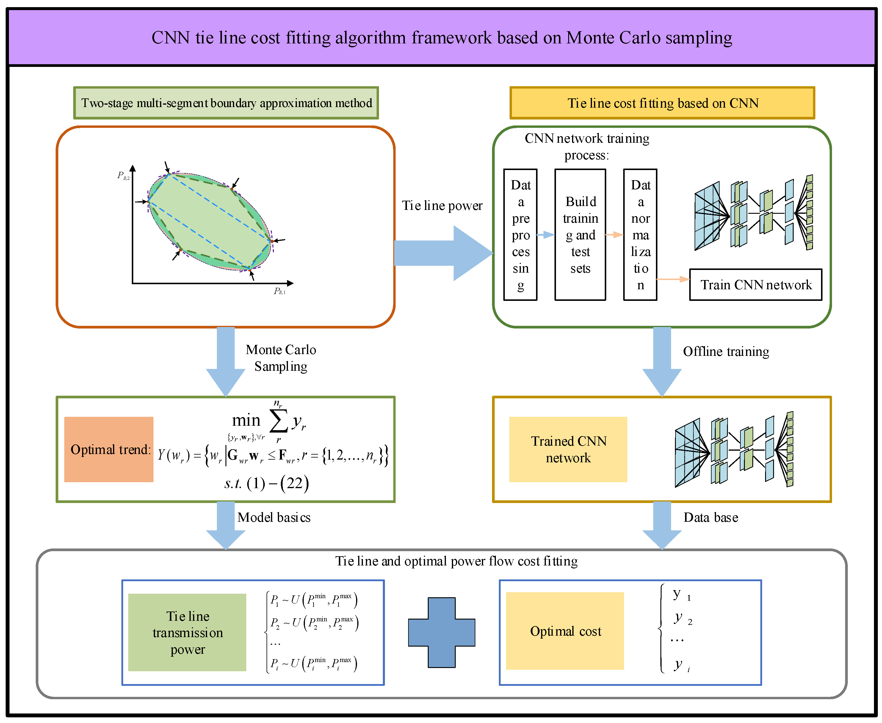
A two-stage multi-segment boundary approximation method (TSM) is proposed to describe the accurate feasible region of tie line power in an AC/DC hybrid distribution network. In the first stage of the TSM method, the linear constraints of the AC/DC hybrid distribution network are iteratively solved to obtain an approximate feasible region. In the second stage, the approximate feasible region of the first stage is modified by nonlinear constraints, and finally, the high-precision approximation of the real feasible region is obtained. Examples demonstrate how the suggested method’s accuracy and speed are significantly better than those of previous approaches.
(2)
A non-iterative coordinated optimization method based on feasible region projection is proposed. Aiming at the problem that the feasible region of tie line transmission power cannot retain cost information, a convolutional neural network (CNN) cost function fitting method is proposed. Through Monte Carlo sampling, the functional relationship between tie line transmission power and operating cost is obtained. Under the premise of protecting information privacy, alternating iteration is avoided, and high-precision coordinated operation of the AC/DC hybrid distribution network system is realized.
The subsequent parts of this article are organized as follows. Section 2 describes the related models of the AC/DC hybrid distribution network. Section 3 introduces the feasible region equivalent method. Section 4 introduces the scheduling framework of interconnected systems based on artificial intelligence. Section 5 gives an example simulation. Section 6 summarizes the results obtained in this study as a conclusion.

2. Materials and Methods

To describe the proposed multi-point approximation method, the AC distribution network model is first mathematically modeled. Then, the DC distribution network model and the VSC steady-state model are modeled. The hybrid distribution network schematic is shown in Figure 1.

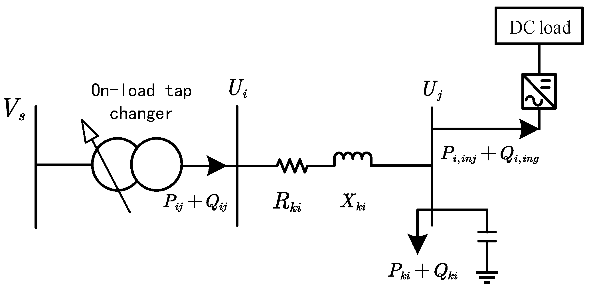
2.1. AC Network Modeling

2.1.1. AC Power Flow Equation

j M i P i j k N i P k i I k i 2 R k i + P B , i = P i , i nj j M i Q i j k N i Q k i I k i 2 X k i = Q i , inj
U j 2 = U i 2 2 P i j R i j + Q i j X i j I i j 2 R i j 2 + X i j 2
I i j 2 U i 2 = P i j 2 + Q i j 2
P i , inj = P i , sub + P i , N M + P AC , i , vsc P AC , i , Load
Q i ,   inj   = Q i ,   sub   + Q i , N M + Q AC , i , vsc Q AC , i ,   Load
In the formula, P i j and Q i j are the branch active power and reactive power of the AC branch i-j, respectively; P B , i represents the active power transmitted by the ith tie line; P i , inj and Q i , inj are the active power and reactive power injected into the AC node i, respectively. I i j is the branch current of the AC branch i-j; U i is the voltage of AC node i; P i , N M and Q i , N M are the active and reactive power outputs of NM node i in the AC power grid, respectively. P AC , i , Load and Q AC , i ,   Load   are the active load and reactive load of AC node i, respectively. P i , sub and Q i ,   sub   are the active and reactive power output of the first end of the AC node i feeder, respectively; Q AC , i , vsc is the reactive power compensated by the AC side node i; P AC , i , vsc is the equivalent injected active power of the converter AC side node i; M i is the terminal node set of the branch with the first node i in the AC power grid; N i is the first node set of the branch with the last node i in the AC power grid; R i j is the resistance of AC branch i-j; X i j is the reactance of AC branch i-j.
Equation (1) is the balance equations of branch active power and reactive power, Equation (2) is the node voltage balance equation, Equation (3) is the node apparent power balance equation, Equations (4) and (5) are the balance equations of active power and reactive power injected into nodes.

2.1.2. AC Distribution Network Security Constraints

P i , sub , min P i , sub P i , sub , max Q i , sub , min Q i , sub Q i , sub , max
P i j 2 + Q i j 2 S i j , max 2
P i , N M = P i , N M , max
Q AC , i , N M = P AC , i , N M tan φ
U min U i U i , max
P B , i , min P B , i P B , i , max , i = 1 , 2 , N T
where P i , sub , max and P i , sub , min are the upper and lower limits of the active power output at the head end of the feeder, respectively; Q i , sub , max and Q i , sub , min are the upper and lower limits of the reactive power output at the head end of the feeder; S i j , max is the transmission capacity of AC grid line i-j; P i , N M , max is the upper limit of the active power output of the AC side NM; φ is the power factor angle of NM; U i , max and U min are the upper and lower limits of the AC node I voltage, respectively; P B , i , min and P B , i , max are the limits of the minimum and maximum contact line transmit powers at node i.
Equation (6) is the output constraint at the feeder head end, Equation (7) is the feeder capacity constraint, Equations (8) and (9) are the DG output constraint, and Equation (10) is the node voltage constraint, Equation (11) is the constraint of tie line transmission power. Among them, NM adopts maximum power point tracking (MPPT) control mode, and the power factor is 0.9.

2.2. DC Network Modeling

2.2.1. DC Power Flow Equation

j A i P i j D C k B i P k i D C ( I k i D C ) 2 R k i D C = P i , i n j D C
( U j D C ) 2 = ( U i D C ) 2 2 P i j D C R i j D C + ( I i j D C ) 2 ( R i j D C ) 2
( I i j D C ) 2 ( U i D C ) 2 = ( P i j D C ) 2
P N M , i , inj = P N M , i , N M P N M , i ,   Load  
where P i j D C is the active power of DC branches i-j; P i , i n j D C is the active power injected into DC node i; I i j D C is the current of DC branches i-j; U DC , i is the voltage of DC node i; R i j D C is the resistance of DC branches i-j; A i is the set of end nodes of the branches with the first node of i in the DC network; B i is the set of branches with the end node of i in the DC network the set of first nodes of the DC network; P DC , i , N M is the active output of NM node i of the DC grid; P DC , i ,   Load   is the active load of DC node i.
Equation (12) is the balance equation of the DC branch active power, Equation (13) is the DC node voltage balance equation, Equation (14) is the DC node active power balance equation, Equation (15) is the balance of active power injected into the DC node equation.

2.2.2. DC Distribution Network Security Constraints

P DC , i j P DC , i j , max
P DC , i , N M = P DC , i , N M , max
U DC , i , min U DC , i U DC , i , max
P DC , i , N M is the active output of the DG node i of the DC network; P DC , i ,   Load   is the active load of the DC node i. P DC , i j , max is the transmission capacity of the DC network lines i-j; P DC , i , N M , max is the upper limit of the active output of the DG node i on the DC side; U DC , i , max and U DC , i , min are the upper and lower limits of U DC , i .
Equation (16) is the feeder constraint of the DC grid, Equation (17) is the DC side NM output constraint; Equation (18) is the node voltage constraint.

2.3. Converter Mathematical Model

P AC , VSC , k i I AC , VSC , k i 2 R AC , R = P AC , i , vsc Q AC , VSC , k i I AC , VSC , k i 2 X AC , X = Q AC , i , vsc
P AC , i , vsc = P DC , j i
Q AC , i , vsc , min Q AC , i , vsc Q AC , i , vsc , max
P AC , i , vsc 2 + Q AC , i , vsc 2 S AC , i , vsc , max 2
where P AC , VSC , k i and Q AC , VSC , k i are the active and reactive power output from the AC-side converter branch k i , respectively; I A C , V S C , ki is the current of the AC-side converter branch k i ; R AC , R and X AC , X are the converter equivalent resistance and reactance, respectively; Q AC , i , vsc , max and Q AC , i , vsc , min are the upper and lower limits of Q AC , i , vsc , respectively; and S AC , i , vsc , max is the capacity of VSC.
Equations (19) and (20) are the VSC power flow equation, and Equations (21) and (22) are the reactive power compensation constraints and VSC capacity constraints, respectively.

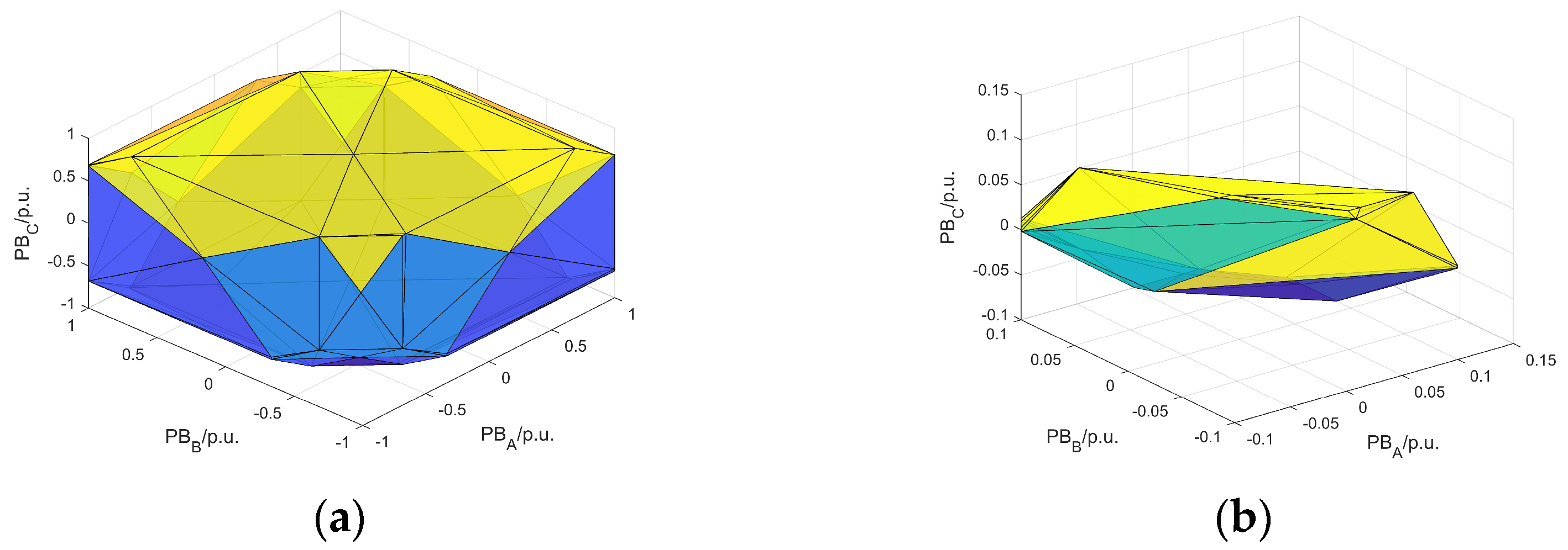
3. Method of Characterization of the Feasible Region of the Tie Line

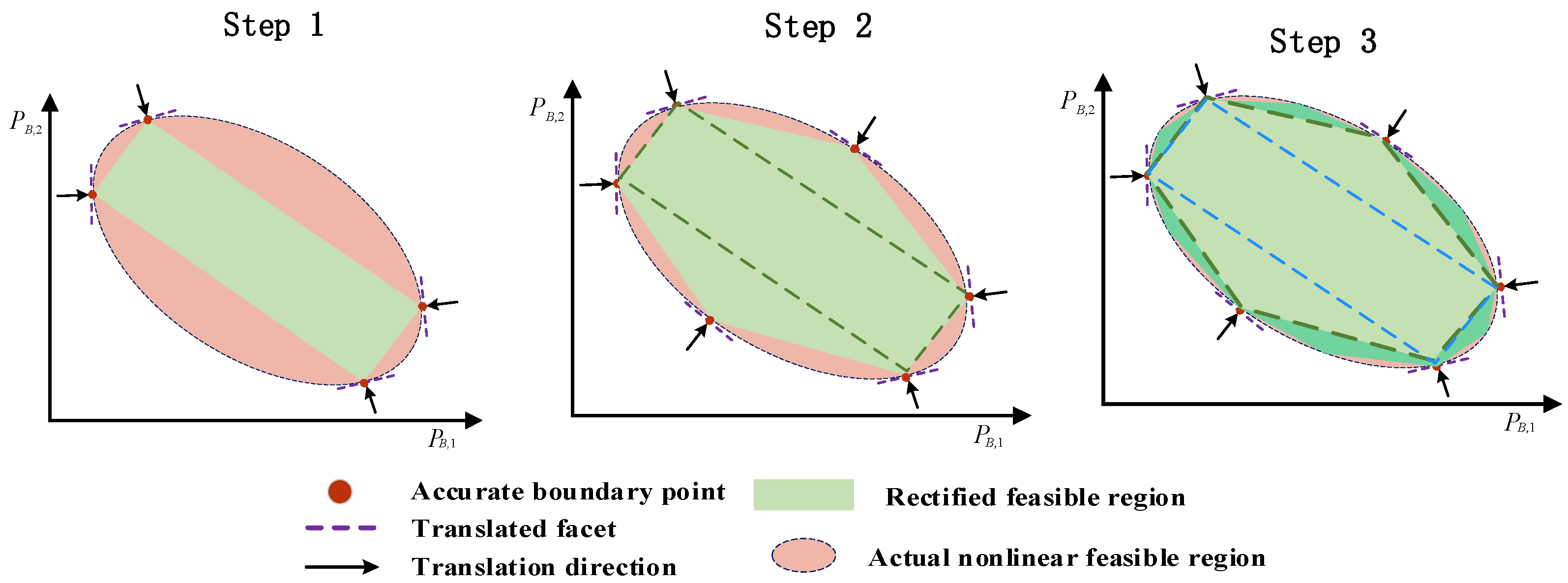
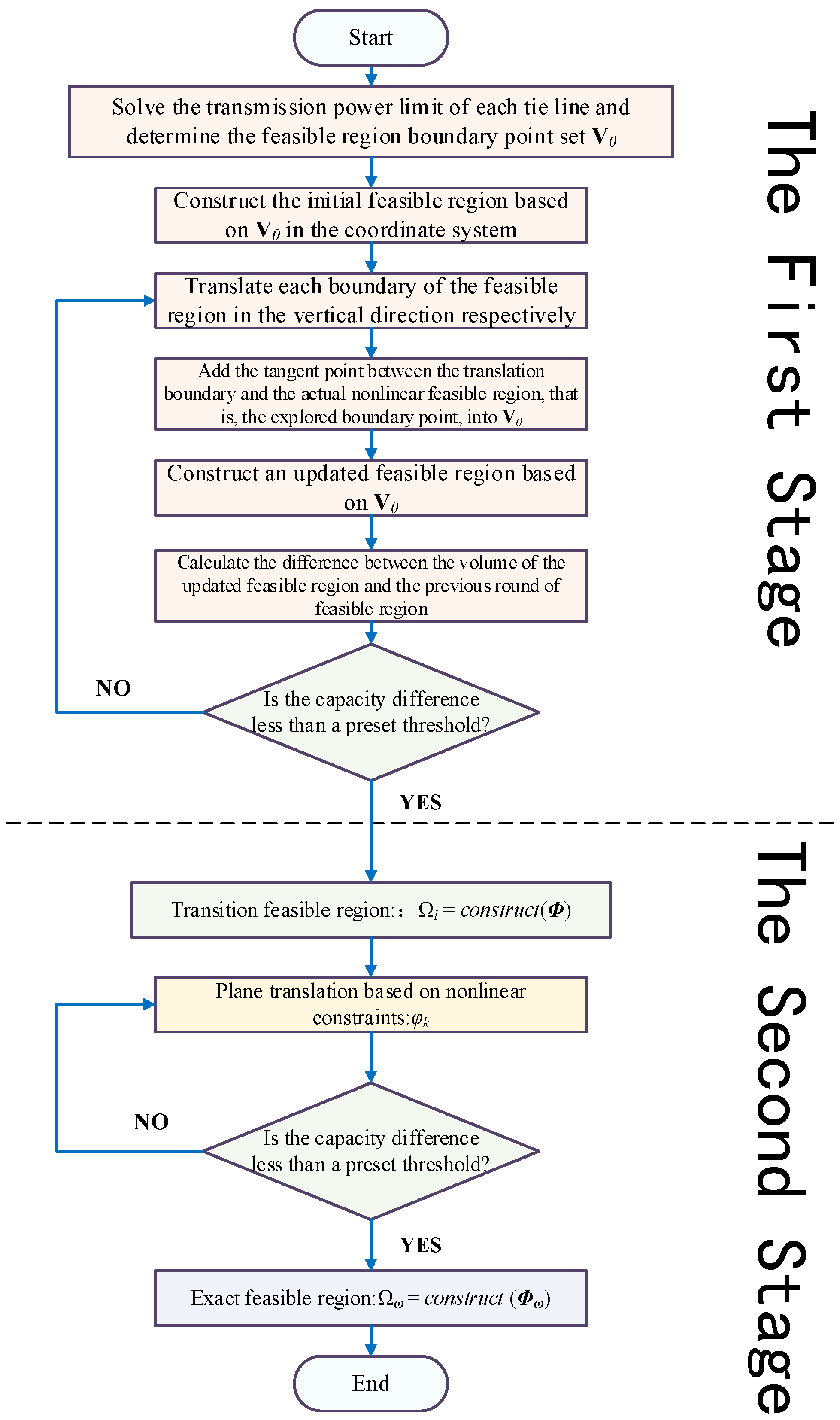
3.1. Search Process of Multi-Segment Boundary Approximation Method

A multi-dimensional polygon called the viable zone of the hybrid distribution network is used to display the tie lines transmission power range. Determining the polygon’s border points is essential to using the multi-segment boundary approximation approach. Figure 2 depicts the flow chart for the multi-segment boundary approximation approach. The fundamental concept is to translate each hyperplane of the existing approximate polyhedron outward in the direction of its normal to seek new boundary points. Then, using the acquired new boundary points and the existing boundary points, a new, more precise approximation polyhedron is created to quickly gather the schedulable area boundary information.
(1)
Initialization of Boundary Points
By exploring the upper and lower limits of each variable in P B = [ P B , 1 , P B , 2 , , P B , i , ] , i = 1 , 2 , N T , the initial boundary points of the approximate feasible region are determined. Two optimization problems are often used to represent the search process for the i-th  P B :
max P B , i s . t .   ( 1 ) 22
min P B , i s . t .   ( 1 ) 22
The above formula’s optimal solutions can be noted as a collection of boundary points to create a first workable zone. It is possible to project the nonlinear restrictions into the feasible area.
(2)
Iteratively updating the approximation polytope
To locate additional boundary points of the feasible region, each of the k hyperplanes must be translated outward along their normal direction during the k-th iteration. The following optimization problem is formulated to find new boundary points for the k-th hyperplane.
Ω k = P B A k P B ρ
(3)
Accuracy Judgement of Multipoint Approximation
The two-stage multi-segment boundary approximation method (TSM) is used to progressively approach the accurate feasible region by repeatedly and continually searching for boundary points. The multi-area volume increment is used to gauge how accurate each iteration estimate is. The iteration ends when the polyhedron’s volume increase falls below the predetermined threshold. The criterion for termination is:
δ V = V ( Ω k + 1 ) V ( Ω k ) V ( Ω k ) ε
where ε denotes a predetermined cutoff point. V ( Ω k ) represents the volume Ω k of the polyhedron in the kth iteration. Two phases expedite the solution procedure for the volume of a polyhedron with n ( n m + 1 ) border points. The first stage involves splitting the resultant polyhedra into nm simplexes, then (23) calculates the volume of each simplex. The total of the volumes of these simplexes may be used to compute the polyhedron’s volume in the second phase. The final feasible region is shown in dark green in Figure 2, Step 3.

3.2. Two-Stage Multi-Segment Boundary Approximation Method (TSM)

The entire identification process is conducted using the nonlinear model, ensuring the reliability of the results. However, the computation can be time-consuming due to the presence of multiple nonlinear iterations. Furthermore, the number of vertex identifications substantially increases as the dimension of the feasible region expands.
To enhance the computing performance, a two-stage multi-segment (TSM) strategy is proposed to quickly and accurately approximate the nonlinear feasible region, as shown in Algorithm 1. The principle of the TSM algorithm is to replace the general nonlinear power flow constraints with simplified linear ones during vertex identification. Although this simplification may introduce some search errors, it could significantly increase computation efficiency. In addition, an error corrective strategy is proposed for boundaries under the simplified condition constraints. The boundaries obtained under the simplified conditions are corrected by the exact system constraints, and the exactly feasible domains under the nonlinear power flow constraints are finally obtained, and the solution speed is greatly improved without affecting the fine reading of the feasible domains.
Algorithm 1: Two-stage multi-segment (TSM)
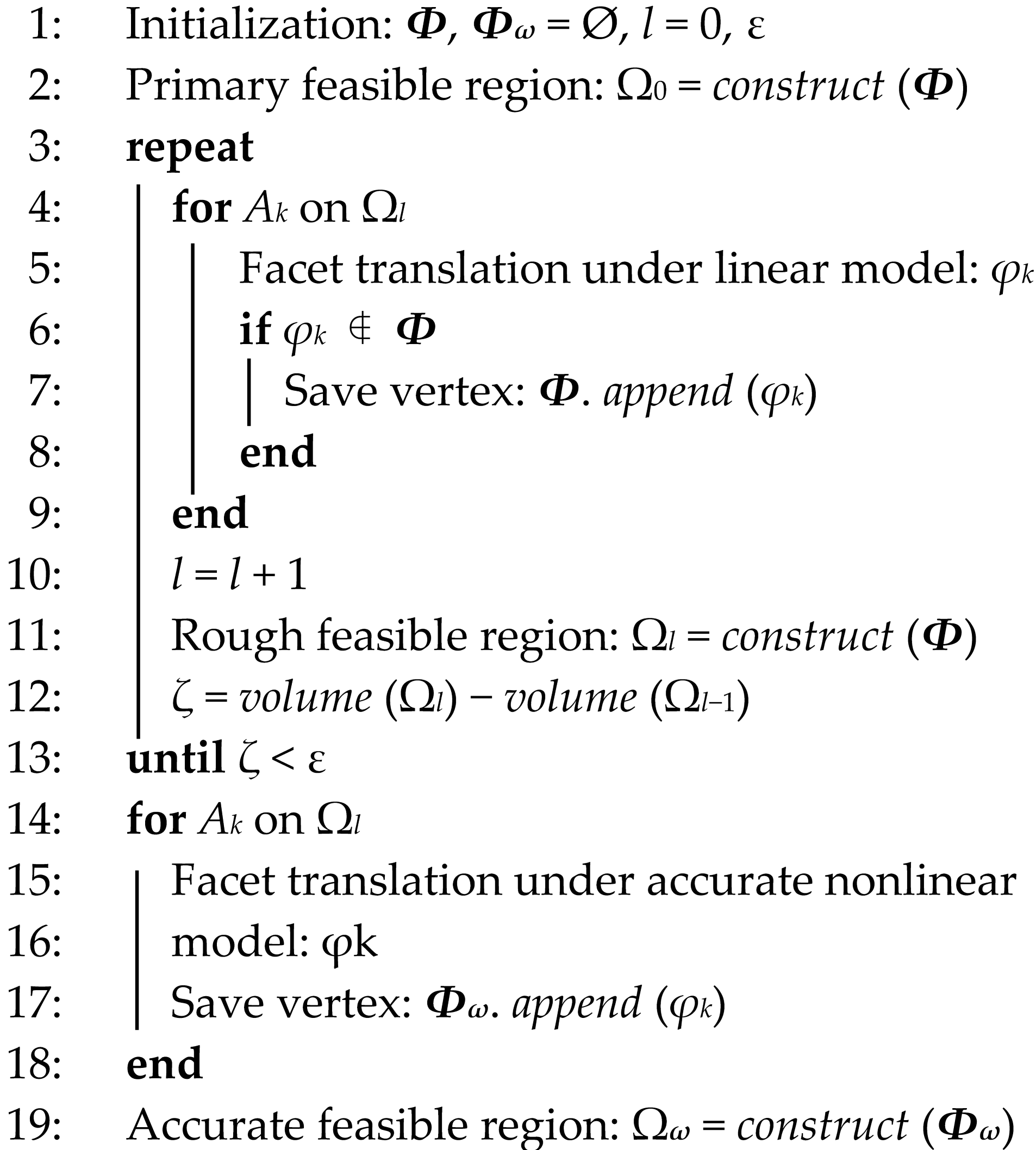
Energies 17 01462 i001
The TSM algorithm has two main stages: orientation and correction. The schematic diagram of the two-level multi-segment boundary is shown in Figure 3. A two-stage approximation strategy is adopted. In the first stage, a linear model is first used for rapid approximation, and linearized power grid constraints are used to quickly and iteratively search for the boundary points of the feasible region. This can greatly improve computational efficiency and quickly obtain a rough approximation of the feasible region. The second stage uses precise nonlinear grid constraints to correct the boundary points obtained in the first stage and modify inaccurate boundary points. Finally, a high-precision feasible region approximation is obtained. Two-stage collaborative work not only ensures accuracy, but also greatly improves the convergence speed. Through the above improvements, the method in this paper has made up for the shortcomings of the traditional linear model to a certain extent, improving the accuracy of feasible domain equivalence. This method provides important support for optimal dispatch and planning of the power grid.
The general idea of the proposed method is as follows:
(1)
First-stage fast approximation. In the first stage, linearized grid constraints are used to quickly and iteratively search for boundary points of the feasible region. This can greatly improve computational efficiency and quickly obtain a rough approximation of the feasible region. The hybrid grid linear model is as follows:
(i)
AC linearized branch power flow model
Using the ratio of power and voltage amplitude as state variables, an AC linearized branch power flow model is proposed:
P ^ i , i n g = j M ( i ) P ^ i j k N ( i ) P ^ k i Q ^ i , i n g = j M ( i ) Q ^ i j k N ( i ) Q ^ k i
W j , ac W i , ac = R k i P ^ i j + X i j Q ^ i j
P ^ i , i n g = P i , i n j W i , ac Q ^ i , i n g = Q i , i n g W i , ac W i , ac = 1 / U i 2 U i
In the formula: W i , ac is the reciprocal of the AC node voltage amplitude; P i , i n j and Q i , i n g are the active and reactive injected power of the AC node i , respectively; P ^ i , i n g and Q ^ i , i n g are the ratios of the active and reactive injected power of the AC node i to the node voltage amplitude, respectively; P ^ i j and Q ^ i j are the active power of the AC branch i j , respectively, and the ratio of reactive power to the voltage amplitude of the first-end node; R k i and X i j are the resistance and reactance of the AC branch i j .
Formula (27) is the node power balance constraint; Formula (28) is the branch voltage drop equation. During the approximation process of the above model, it is assumed that the ratio of the inflow power at the head end of the branch to the voltage amplitude at the head end and the ratio of the outflow power at the end to the voltage amplitude at the end are equal.
  • (ii)
    DC linearized branch power flow model
The DC linearized power flow model is derived based on the AC linearized power flow model. The relationship between the voltage of the first and last nodes of the branch and the power of the branch is as follows:
U i D C U j D C = P i j D C / U i D C R i j D C U j D C U i D C = P j i D C / U j D C R i j D C
In the formula: U i D C is the voltage amplitude of the first node of the DC branch i j ; U j D C is the voltage amplitude of the end node of the DC branch i j ; R i j D C is the resistance of the DC branch i j ; P i j D C and P j i D C are the active power flowing from the first end of the DC branch i j to the end and from the end to the first end, respectively.
By adding the first and second formulas of formula (30):
P ^ i j D C = P i j D C / U i D C = P i j D C / U j D C = P ^ j i D C
In the formula: P ^ i j D C is the ratio of the active power of the DC branch i j to the node voltage amplitude.
The DC node power balance equation is:
P N M , i , N M = j M i P N M , j , i n g + k N i P N M , k , L o a d
Divide the voltage amplitude of the node i on both sides of Equation (32) at the same time and bring it into Equation (33) to obtain the DC power balance equation:
P ^ N M , i , N M = j M i P ^ N M , j , i n g k N i P ^ M N , k , L o a d
Further, expand the Taylor expansion of the reciprocal of the node voltage amplitude near 1 and ignore the higher-order terms:
W i , dc = 1 / U i D C 2 U i D C
In the formula: W i , dc is the reciprocal of the DC node voltage amplitude.
Bringing it into Equation (34), the DC branch voltage drop equation is:
W j , dc W i , dc = P ^ i j D C R i j D C
Therefore, the DC linearized power flow model under this set of state variables is:
P ^ i , i n g = j A i P ^ i j D C k B i P ^ k i D C W j , dc W i , dc = P ^ i j D C R i j D C
  • (iii)
    VSC linearized model
P ^ A C , V S C , k i = P ^ A C , i , v s c Q ^ A C , V S C , k i = Q ^ A C , i , v s c W k , c W k , s = P ^ A C , V S C , k i R A C , R + Q ^ A C , V S C , k i X A C , X
In the formula: P ^ A C , V S C , k i and Q ^ A C , V S C , k i are the ratios of the active and reactive power injected into the VSC by the AC bus and the voltage amplitude, respectively; P ^ A C , i , v s c and Q ^ A C , i , v s c are the ratios of the active and reactive power injected into the VSC by the AC side virtual node and the voltage amplitude, respectively; W k , s and W k , c are the AC bus and The reciprocal of the virtual node voltage amplitude, respectively.
(2)
The second stage of precise correction. The rough feasible region obtained in the first stage may have certain errors. The second stage uses precise nonlinear grid constraints to correct the boundary points obtained in the first stage and modify inaccurate boundary points. Finally, a high-precision feasible region approximation is obtained. Two-stage collaborative work not only ensures accuracy, but also greatly improves the convergence speed.

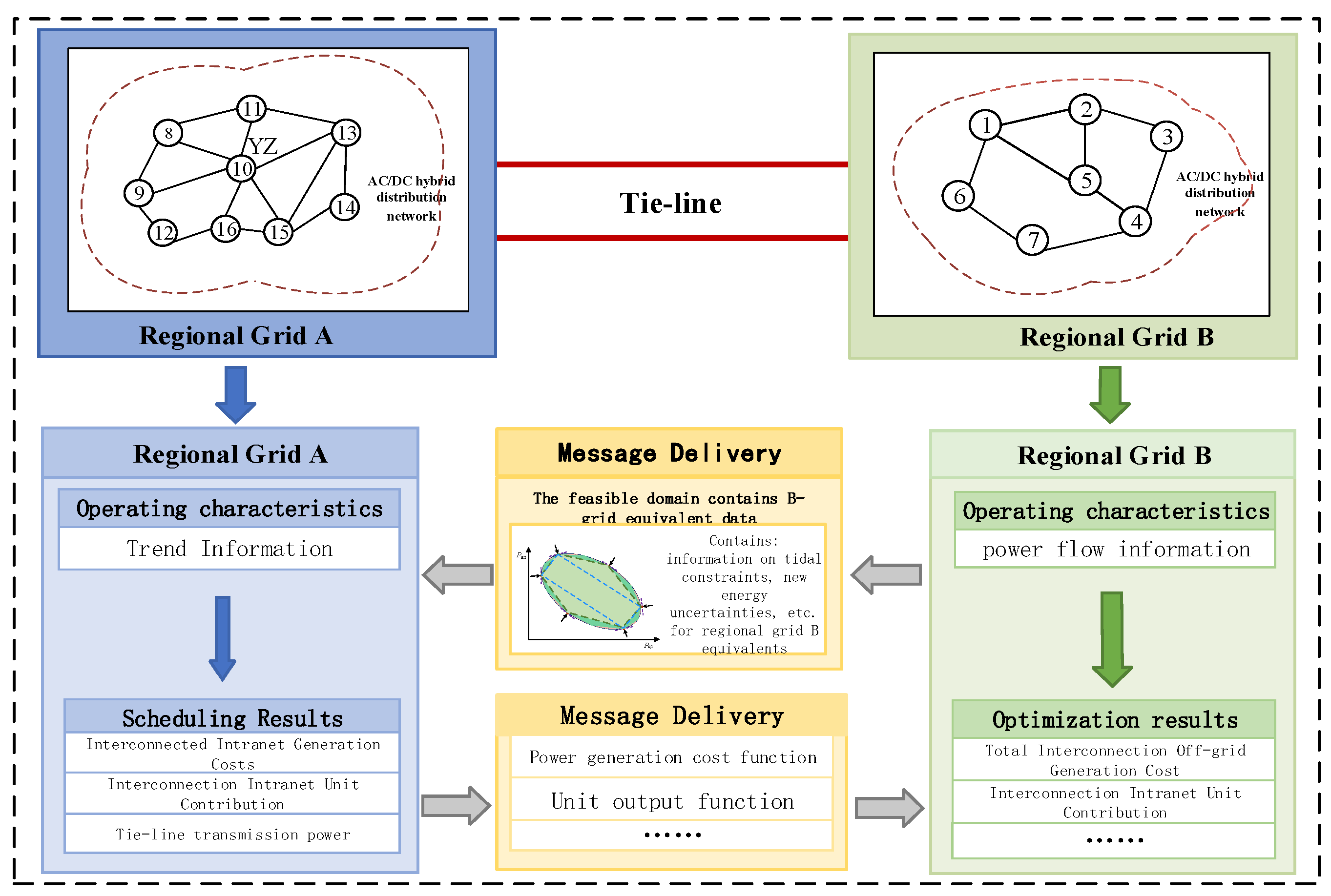
4. Artificial Intelligence-Based Scheduling Framework for Interconnected Systems

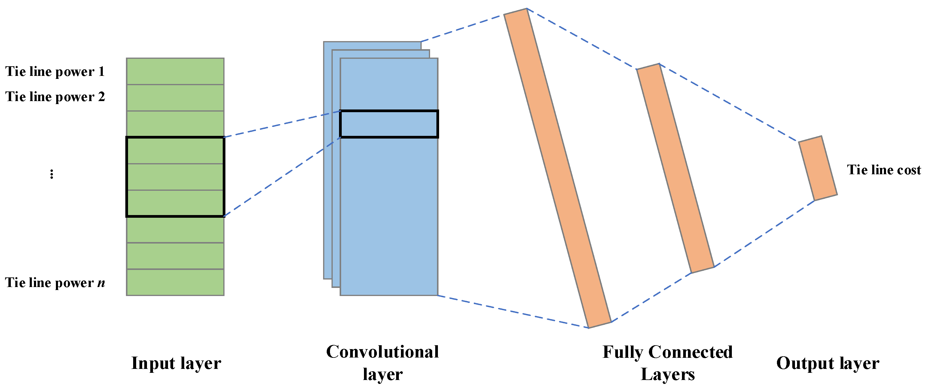
4.1. Convolutional Neural Network Model

The data set of CNN is generated using the Monte Carlo method. The construction process of the training sample set based on the Monte Carlo method can be described as follows: Firstly, a large number of tie line power operating points are generated according to uniform probability distribution, that is:
P 1 U P 1 min , P 1 max P 2 U P 2 min , P 2 max P i U P i min , P i max
The two-stage multi-segment boundary approximation method is used to calculate the feasible region of the transmission power of the tie line of the hybrid distribution network. The optimal power flow of the distribution network is calculated by the transmission power of the tie line in the feasible area. The objective function is:
min i S G a 2 i P G i 2 + a 1 i P G i + a 0 i ,   i S B
s . t .   ( 1 ) 22
In the formula, P G i is the active power output of the generator set on node i; S B is the set of nodes; a 0 i , a 1 i , and a 2 i are the parameters of the consumption characteristic curve.
Through the optimal power flow calculation, the training sample set of network operation states including each node voltage parameter, branch power parameter, tie line power, and network operation cost can be obtained. Further classification of the obtained training sample set can provide a basis for the subsequent training of convolutional neural networks (CNN).
An input layer, an output layer, convolutional layers, fully connected layers, etc., make up a CNN, as shown in Figure 4. The convolutional layer achieves feature extraction by convolving the input array with convolutional kernels, where the kernel slides over the input array in a window-like manner, performing convolutional operations on each window to generate a feature array. The parameters of the convolutional layer include the kernel size, stride, padding method, and number of kernels. The fully connected layer classifies or regresses the features extracted from the convolutional layer. Its output is the predicted result of the model, which can be compared with the ground truth to compute the loss and perform optimization.
The CNN can be expressed by the following formula.
h c = ReLU X W c + b c
h f c = h c × W f c + b f c
where X is the convolution layer input vector, Wc is the weight matrix of the convolution kernel, and bc is the corresponding bias; convolution is indicated by the asterisk (*); the rectified linear unit activation function (ReLU) with nonlinear transformation; hc is the feature map generated by the convolution layer; Wfc and bfc are the weights and bias of the fully-connected layer, respectively, and hfc is the output of the fully-connected layer.
Overall, the input-output relation of the CNN is expressed as
C l = f θ P l
where Pl and Cl denote the tie line transmission power vector and the network operating cost for the l-th sample, respectively. The training procedure of CNN is as follows. Initially, the mini-batch gradient descent approach is used to train the CNN. Subsequently, the ad-am optimizer modifies the CNN’s parameters (θ) to minimize the Root Mean Square Error (RMSE) between the actual output and the anticipated output, taking into account the weights and biases in each layer. We were able to retrieve the trained CNN parameters after many trainings.
As shown in Figure 5, the CNN tie line cost fitting algorithm based on Monte Carlo sampling proposed in this article is mainly divided into two steps: Monte Carlo sampling and CNN cost fitting. On the data side, Monte Carlo sampling forms a data set. First, an accurate feasible region model is obtained according to the two-stage multi-segment boundary method. The points in the feasible region represent the output of the tie line. Through Monte Carlo sampling, a set of tie lines is obtained. The output power is substituted into the optimal power flow to obtain the optimal cost of the AC-DC hybrid distribution network. Through multiple samplings, the historical data set of the power and optimal cost of the AC-DC hybrid distribution network tie line is obtained, and then a convolutional neural network is used to learn it, and finally, a more accurate regression prediction network is generated. The model side is the optimization solution part. The trained neural network is used to perform non-iterative scheduling of the AC and DC hybrid distribution network, which effectively protects the privacy of the power grid and avoids the problem of long alternating iteration times.

4.2. Cost Fitting of Feasible Region of Tie Line in AC/DC Hybrid Power Grid Based on Convolutional Neural Network (CNN)

Through the convolutional neural network (CNN), the expression of the boundary of the feasible region of the transmission power of the tie line and the cost function of the coordinated dispatch of the interconnected power grid in the feasible region of the transmission power of the tie line can be obtained. Based on the data provided previously, this part uses a feasible region and a cost function to fit. The tie line coupling variable w is then utilized as the optimization variable to minimize the overall cost of economic dispatch for each regional power grid. Specifically, this means that:
min   y r , w r , r r n r y r
Y ( w r ) = w r G w r w r F w r , r = 1 , 2 , , n r
s . t .   ( 1 ) ( 22 )
The economic dispatch cost variable of the rth regional power grid is represented by y r , and the expression relationship of the coupling variable r in the feasible area of the tie line transmission power in the region is described by the G w r , F w r matrices and vectors. The overarching goal of scheduling is to reduce each regional system’s scheduling cost, as shown by Equation (44). The transmission power of the tie line of the regional power grid’s feasible region limitation is described by the Equation (45).
Reliable dispatch decisions can be derived from the tie line transmission power feasible region. Additionally, interconnected grid data privacy is safeguarded and sensitive information leakage is prevented through coordination based on this feasible region. Figure 6 depicts the coordination process based on feasible region mapping. Regional grid B’s important dispatch information is mapped to the tie line transmission power feasible area, considering power flow and new energy uncertainty in the interconnected grid. Mapped information includes comparable power flow limits, new energy uncertainty, and production costs for regional grid B within the feasible region. Data privacy may be preserved since mapped information excludes grid B’s specific data. To achieve coordination and complementary energy resources, mapped information is given to regional grid A. This allows grid A to coordinate scheduling while considering grid B’s operational characteristics.
The two-level multi-segment boundary approximation method is based on the fully nonlinear power flow constraints of the hybrid network and accurately captures the feasible region of the tie line power flow. The feasible region is an accurate representation of the system’s safety constraints and limitations. Through the two-stage multi-segment boundary approximation method, the feasible region of the tie line can be quickly and accurately characterized. An accurate feasible region prevents tie lines used to transmit power from violating any voltage, power, or other limits that could compromise safety. CNN-based cost mapping is based on accurate feasible regions when optimizing economic dispatch. The dispatch solution must satisfy the tie line power flow constraints characterized by the feasible region model. The non-iterative coordinated dispatch method ensures that only safe operating points are identified and dispatched in the AC/DC hybrid distribution system by fully incorporating nonlinear network models and constraints into feasible region characterization and coordinated dispatch. Safety constraints are adhered to at every stage from modeling to optimization.

5. Case Studies

In this example, the improved IEEE 33-section AC/DC distribution network system is used. The AC grid voltage level is 10 kV, the DC grid voltage level is ± 10 kV, the converter station capacity is 4 MVA, and the feeder capacity is 4 MVA. Taking the IEEE 33-bus double contact line system as an example, the efficiency of the two-stage multi-segment boundary acceleration identification technology and the multi-segment boundary approximation method is verified. In addition, two IEEE 33-bus systems are used to confirm the effectiveness of the proposed scheduling strategy. It is characterized by feasible areas associated with tie lines 3, 9 and 12. The above system is considered as part of a larger regional network connected to other networks, as shown in Figure 7.
In order to verify the effectiveness of the two-stage multi-segment boundary approximation method and the non-iterative coordinated scheduling method proposed in this chapter, the example simulation in this section is performed on Windows 10 system, the CPU is Inter(R) Core(TM) i5-5200U (Intel Corporation, Santa Clara, CA, USA), and the main frequency is 2.7 GHz. In a test environment with a main memory of 16 GB, it is based on MATLAB 2017b software and YALMIP general modeling platform, and uses IBM CPLEX 12.8 and IPOPT commercial solver for solving.

5.1. Simulation Setup and Comparison Methods

Three assessment techniques are set up to capture PB to demonstrate the usefulness of the suggested approaching tie line method. M0 is used as the reference method for comparison.
M0: Monte Carlo simulation experiment.
M1: Maximum capacity method expansion.
M2: Proposed a way for searching boundary points.
By checking for accuracy and efficiency, the viability of the feasible region equivalent model of tie line transmission power is confirmed. Accuracy (CR), error rate (ER), and running time (T) were defined as assessment indicators and statistical tests were carried out using 6000 test points. The results are shown in Figure 8.
Table 1 that follows displays the effectiveness of the three distinct approaches, taking into account both computational correctness and efficiency. In particular, M1 and M2 had CR values of 53.56% and 99.78%, respectively, and ER values of 0% and 0.04%. This result shows that there is no misjudgment of the infeasible locations, but the M2 is substantially lacking in accuracy for the feasible points. Furthermore, a small number of unfeasible spots are underestimated, and places meeting the operational restrictions of heat networks are essentially included in the viable zone denoted by M2. We may infer that M2 is the best approximation of the real viable area.

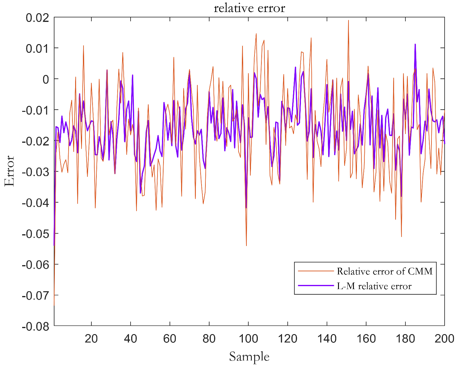
5.2. CNN-Based Cost Function Fitting

For the AC and DC hybrid distribution network, there are only 6 non-zero input data, which is a small calculation example system. In order to prevent the network from being too deep and causing over-fitting of the results, this paper sets up a three-layer convolution network, with the number of convolution kernels being 16 and 16, respectively. 32 and 64, size 3 × 1. In order to speed up the training and reduce the sensitivity of the initialization parameters, this paper inserts a batch normalization layer between the convolution layer and the pooling layer to make the data more regular. Finally, the model undergoes three convolution and three pooling operations to compress the input data into a one-dimensional vector, and extract features through a fully connected layer. A network structure with a large top and small bottom similar to the shape of an inverted pyramid is more conducive to learning. Therefore, the two-layer fully connected layer designed in this article has the number of neurons in sequence of 128 and 32. Finally, it is connected to the fully connected layer whose output parameters correspond to the number of neurons and outputs a vector in the specified format. The network information is as shown in Table 2.
In this section, the convolutional neural network (CNN) is compared with the deep neural network (DNN) to prove the superiority of the convolutional neural network (CNN).
M0: DNN-based cost function fitting
M1: CNN-based cost function fitting.
Table 3 displays the performance comparison of the deep neural network (DNN) approach with the suggested method. The proposed CNN-based technique outperforms the DNN method in terms of performance. The CNN approach has far less root mean square error (RMSE) and mean absolute percentage error (MAPE) than the DNN method. Additionally, the CNN method’s R2 is significantly greater than the DNN neural network technique’s, and its fitting accuracy is higher. Figure 9 displays the relative error comparison between CNN and DNN.

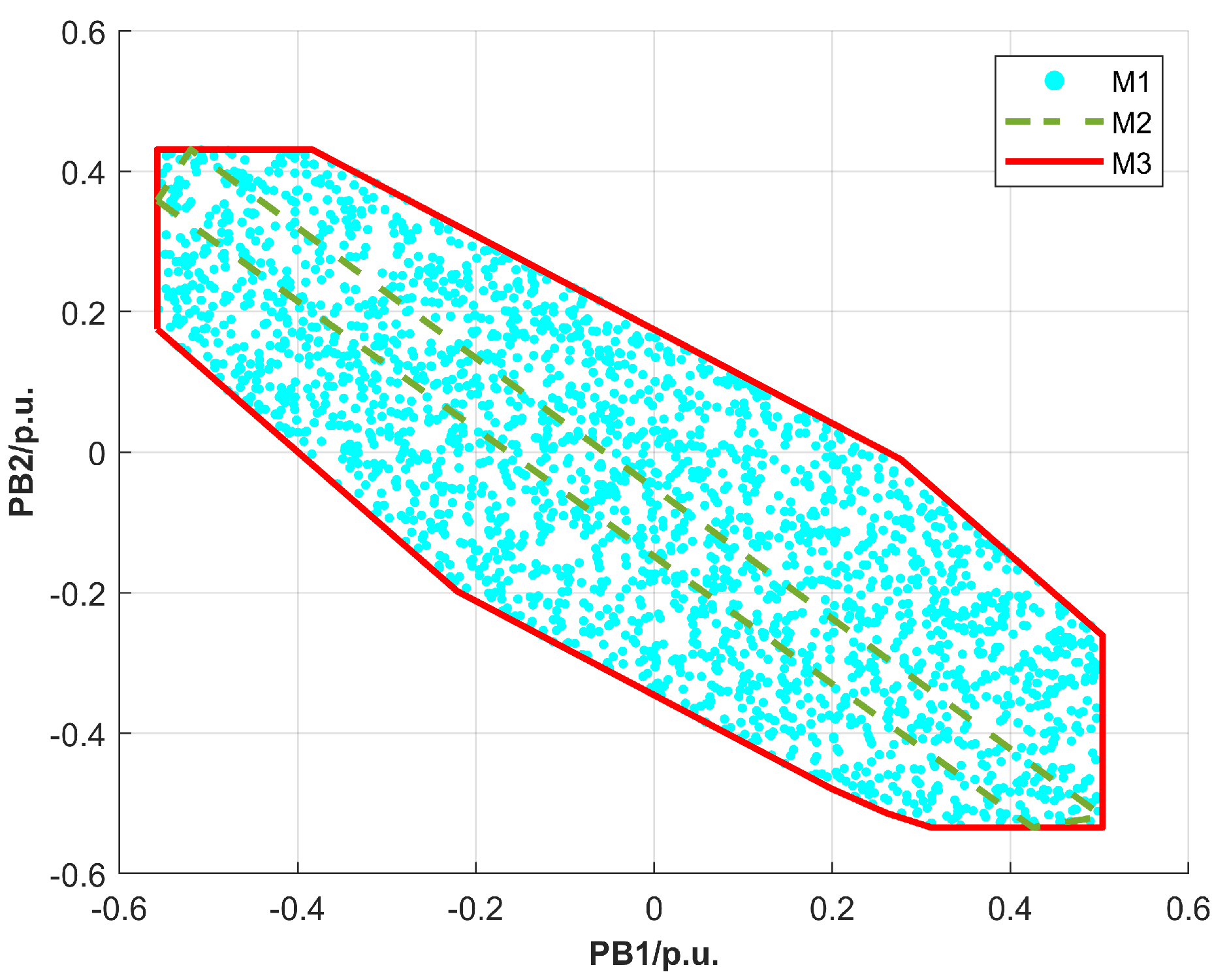
5.3. A Paradigm for Dispatching Interconnected Systems That Take into Account the Practical Range of AC/DC Hybrid Power Grid Transmission

As seen in Figure 10, this part builds a two-region linked power grid based on the basic IEEE 33-node system and the improved IEEE 33-node system. Among them, Area 1 and Area 2 transmit power through the three boundary nodes connected to the tie lines, respectively. P B 1 to P B 3 represent the active power transmitted on these 3 tie lines.
In this section, the proposed collaboration method is compared with centralized, distributed, and multi-parameter planning methods. Centralized scheduling is used as a benchmark to verify the accuracy of the scheduling results.
M0: Centralized scheduling method
M1: Distributed scheduling method
M2: Scheduling method based on multi-parameter programming mapping feasible region
M3: The approach suggested in this article
This article compares the current centralized dispatch system with the interconnected power grid coordinated dispatch approach, which is based on the feasible area of tie line transmission power. Table 2 displays the results of the computation.
Each tie line’s transmission power is within the practical range, as Table 4 demonstrates. The scheduling is matched with the centralized scheduling result based on the suggested viable area of tie line transmission power. This allows for the proper formulation of the tie line transmission scheme within the practical range. The border of the tie line transmission’s viable area may be precisely mapped to the internal operating limits of the regional power grid using this approach. The M1 method’s accuracy is somewhat less accurate. This technique aims to thoroughly characterize the operating area while taking power flow and tie line cost limits into account. Coordination outcomes might vary if M1 data is not synced. Since M2 uses a linear model and the feasible region’s precision is low, deviation results will be obtained.
Compared with single-region dispatch, multi-region AC and DC hybrid distribution networks achieve lower power generation costs, as Table 5 demonstrates. Compared with M1 and M2, the cost of the method proposed in this article (M3) is reduced by US$2043 and US$1653, respectively. Compared with the real optimal solution of centralized collaborative optimization (M0), the optimality gap of the proposed method (M3) for the test system is very small, 0.01725%. This verifies that the proposed equivalent flexibility model can accurately represent external network constraints to achieve near-global optimal economic dispatch. Computational efficiency: The proposed non-iterative scheduling method reduces the solution time of the IEEE-33 bus system by 53.524 s and 44.751 s compared to M1 and M2, respectively, demonstrating practical computational advantages while maintaining a near-optimal solution. In summary, the simulation case study validates the proposed approach: (1) reduces costs and improves social welfare compared to single-region dispatch, (2) ensures feasible stable grid operation by respecting operational constraints, (3) achieves near-centralized. The global optimal solution is collaboratively optimized, (4) providing computing acceleration and protecting data privacy. These results demonstrate the effectiveness of the proposed non-iterative coordinated optimization method.
In terms of solving dispatch costs, the M0 method uniformly models the interconnected distribution network based on comprehensive network data of the distribution network. Although it obtains accurate dispatch costs of the interconnected distribution network, it fails to protect the data privacy of the regional power grid. Actual power grid operation information involves sensitive issues such as operational interests and security, making it difficult to implement the M0 method. Although the M1 method can protect the privacy of the operator, the solution time and accuracy are not high. Although the accuracy of the M2 method is greatly improved compared to the M1 method, the solution time is longer. The M3 method sacrifices a small amount of solution time to obtain cost-mapping information essential for dispatch. The established coordinated dispatch model can effectively protect data privacy within the regional power grid. In summary, the proposed method can well balance the solution accuracy and efficiency of coordinated dispatching of interconnected distribution networks and protect data privacy.

6. Conclusions

The complementarity and flexibility between regional power grids can be utilized to the greatest extent, thereby improving the optimal allocation and utilization of power resources. By characterizing the power between regional grids, the grid can be made to operate more economically. At the same time, collaborative optimization is carried out on the premise of protecting the commercial confidentiality of the regional power grid. The paper uses the connected line power to represent the constraints of the external power grid through the equivalent flexibility model, avoiding the leakage of detailed data. A safe and feasible economic dispatch plan can be obtained. The two-stage multi-segment boundary approximation method proposed in this paper considers power balance constraints, line power flow constraints, generation capacity, and other constraints, and avoids unsafe dispatch results that may be caused by nonlinear constraints. The non-iterative scheduling method can reduce the communication cost and computational burden caused by data exchange. Compared with centralized and distributed optimization methods that require a large amount of data exchange and iterative calculations, the paper can be solved with only one data exchange through the equivalent model. Accurately describing the power exchange capabilities between regional power grids can maximize the complementarity and synergy between power grids and obtain economical and safe dispatch solutions while protecting the commercial confidentiality of regional power grids. This is of great significance for achieving cross-regional joint optimal dispatch in the context of the current power system reform and the large-scale integration of new energy into the power grid.
The outcomes of the simulation show how successful the suggested collaboration strategy is. In contrast to the centralized strategy, the collaborative approach that has been suggested can provide satisfactory sub-optimal results while safeguarding the privacy of regional grids and minimizing the need for excessive information sharing amongst them.
Outlook: For complex multi-region coordinated optimization problems, this method may face the following challenges: when the number of regional networks increases, the number of boundary points will exponentially increase, and the amount of calculation will significantly increase. This requires more efficient algorithms and hardware to deal with. The greater the difference in network structure and parameters between different regions, the approximation accuracy will decrease. The next step of research will be to improve both the algorithm and the model to increase its application scale.

Author Contributions

Conceptualization, W.D.; Methodology, Y.G.; Software, H.H.G.; Validation, Z.Z.; Formal analysis, Y.L.; Data curation, J.J. All authors have read and agreed to the published version of the manuscript.

Funding

This research was funded by National Natural Science Foundation of China under grant 512No.52107082 and Specific Research Project of Guangxi for Research Bases and Talents under grant 513No.AD22080052.

Data Availability Statement

The raw data supporting the conclusions of this article will be made available by the authors on request.

Conflicts of Interest

Author Jiangyi Jian was employed by the company Zigong Power Supply Bureau, Sichuan Power Grid Co., Ltd. The remaining authors declare that the research was conducted in the absence of any commercial or financial relationships that could be construed as a potential conflict of interest.

References

  1. Huang, H.; Zhou, M.; Zhang, S.; Zhang, L.; Li, G.; Sun, Y. Exploiting the Operational Flexibility of Wind Integrated Hybrid AC/DC Power Systems. IEEE Trans. Power Syst. 2020, 36, 818–826. [Google Scholar] [CrossRef]
  2. Xiao, H.; Pei, W.; Deng, W.; Ma, T.; Zhang, S.; Kong, L. Enhancing risk control ability of distribution network for improved renewable energy integration through flexible DC interconnection. Appl. Energy 2021, 284, 116387. [Google Scholar] [CrossRef]
  3. Sarangi, S.; Sahu, B.K.; Rout, P.K. Distributed generation hybrid AC/DC microgrid protection: A critical review on issues, strategies, and future directions. Int. J. Energy Res. 2020, 44, 3347–3364. [Google Scholar] [CrossRef]
  4. Ertugrul, N.; Abbott, D. DC is the Future [Point of View]. Proc. IEEE 2020, 108, 615–624. [Google Scholar] [CrossRef]
  5. Zhao, J.; Wu, Z.; Long, H.; Sun, H.; Wu, X.; Chan, C.; Shahidehpour, M. Optimal Operation Control Strategies for Active Distribution Networks under Multiple States: A Systematic Review. J. Mod. Power Syst. Clean Energy 2023. Available online: https://ieeexplore.ieee.org/abstract/document/10355075 (accessed on 6 February 2024).
  6. Dong, Y.; Shan, X.; Yan, Y.; Leng, X.; Wang, Y. Architecture, Key Technologies and Applications of Load Dispatching in China Power Grid. J. Mod. Power Syst. Clean Energy 2022, 10, 316–327. [Google Scholar] [CrossRef]
  7. Biskas, P.; Bakirtzis, A.; Macheras, N.; Pasialis, N. A Decentralized Implementation of DC Optimal Power Flow on a Network of Computers. IEEE Trans. Power Syst. 2005, 20, 25–33. [Google Scholar] [CrossRef]
  8. Gil-González, W.; Montoya, O.D.; Grisales-Noreña, L.F.; Cruz-Peragón, F.; Alcalá, G. Economic dispatch of renewable generators and BESS in DC microgrids using second-order cone optimization. Energies 2020, 13, 1703. [Google Scholar] [CrossRef]
  9. Kalakova, A.; Nunna, H.S.V.S.K.; Jamwal, P.K.; Doolla, S. A Novel Genetic Algorithm Based Dynamic Economic Dispatch With Short-Term Load Forecasting. IEEE Trans. Ind. Appl. 2021, 57, 2972–2982. [Google Scholar] [CrossRef]
  10. Ellahi, M.; Abbas, G. A Hybrid Metaheuristic Approach for the Solution of Renewables-Incorporated Economic Dispatch Problems. IEEE Access 2020, 8, 127608–127621. [Google Scholar] [CrossRef]
  11. Liu, Y.; Ćetenović, D.; Li, H.; Gryazina, E.; Terzija, V. An optimized multi-objective reactive power dispatch strategy based on improved genetic algorithm for wind power integrated systems. Int. J. Electr. Power Energy Syst. 2022, 136, 107764. [Google Scholar] [CrossRef]
  12. Dey, B.; Bhattacharyya, B.; Márquez, F.P.G. A hybrid optimization-based approach to solve environment constrained economic dispatch problem on microgrid system. J. Clean. Prod. 2021, 307, 127196. [Google Scholar] [CrossRef]
  13. Wang, J.; Peng, Y. Distributed optimal dispatching of multi-entity distribution network with demand response and edge computing. IEEE Access 2020, 8, 141923–141931. [Google Scholar] [CrossRef]
  14. Zhao, J.; Zhang, Q.; Liu, Z.; Wu, X. A Distributed Black-Start Optimization Method for Global Transmission and Distribution Network. IEEE Trans. Power Syst. 2021, 36, 4471–4481. [Google Scholar] [CrossRef]
  15. Li, X.; Zeng, Y.; Lu, Z. Decomposition and coordination calculation of economic dispatch for active distribution network with multi-microgrids. Int. J. Electr. Power Energy Syst. 2022, 135, 107617. [Google Scholar] [CrossRef]
  16. Hou, J.; Zhai, Q.; Zhou, Y.; Guan, X. A Fast Solution Method for Large-Scale Unit Commitment Based on Lagrangian Relaxation and Dynamic Programming. IEEE Trans. Power Syst. 2023, 39, 3130–3140. [Google Scholar] [CrossRef]
  17. Qader, M.R. Power management in a hydrothermal system considering maintenance using Lagrangian relaxation and augmented Lagrangian methods. Alex. Eng. J. 2022, 61, 8177–8188. [Google Scholar] [CrossRef]
  18. Maneesha, A.; Swarup, K.S. A survey on applications of Alternating Direction Method of Multipliers in smart power grids. Renew. Sustain. Energy Rev. 2021, 152, 111687. [Google Scholar] [CrossRef]
  19. Lu, X.; Yin, H.; Xia, S.; Zhang, D.; Shahidehpour, M.; Zhang, X.; Ding, T. A Real-Time Alternating Direction Method of Multipliers Algorithm for Nonconvex Optimal Power Flow Problem. IEEE Trans. Ind. Appl. 2020, 57, 70–82. [Google Scholar] [CrossRef]
  20. Sun, S.; Fu, J.; Wei, L.; Li, A. Multi-objective optimal dispatching for a grid-connected micro-grid considering wind power forecasting probability. IEEE Access 2020, 8, 46981–46997. [Google Scholar] [CrossRef]
  21. Sun, S.; Wang, C.; Wang, Y.; Zhu, X.; Lu, H. Multi-objective optimization dispatching of a micro-grid considering uncertainty in wind power forecasting. Energy Rep. 2022, 8, 2859–2874. [Google Scholar] [CrossRef]
  22. Shang, Y.; Liu, M.; Shao, Z.; Jian, L. Internet of smart charging points with photovoltaic Integration: A high-efficiency scheme enabling optimal dispatching between electric vehicles and power grids. Appl. Energy 2020, 278, 115640. [Google Scholar] [CrossRef]
  23. Tang, K.; Dong, S.; Ma, X.; Lv, L.; Song, Y. Chance-Constrained Optimal Power Flow of Integrated Transmission and Distribution Networks With Limited Information Interaction. IEEE Trans. Smart Grid 2020, 12, 821–833. [Google Scholar] [CrossRef]
  24. Lin, W.; Jin, X.; Jia, H.; Mu, Y.; Xu, T.; Xu, X.; Yu, X. Decentralized optimal scheduling for integrated community energy system via consensus-based alternating direction method of multipliers. Appl. Energy 2021, 302, 117448. [Google Scholar] [CrossRef]
  25. Chen, Z.; Li, Z.; Guo, C.; Wang, J.; Ding, Y. Fully Distributed Robust Reserve Scheduling for Coupled Transmission and Distribution Systems. IEEE Trans. Power Syst. 2020, 36, 169–182. [Google Scholar] [CrossRef]
  26. Zhou, H.; Erol-Kantarci, M.; Liu, Y.; Poor, H.V. A Survey on Model-Based, Heuristic, and Machine Learning Optimization Approaches in RIS-Aided Wireless Networks. IEEE Commun. Surv. Tutor. 2023. [Google Scholar] [CrossRef]
  27. Wang, F.; Xuan, Z.; Zhen, Z.; Li, K.; Wang, T.; Shi, M. A day-ahead PV power forecasting method based on LSTM-RNN model and time correlation modification under partial daily pattern prediction framework. Energy Convers. Manag. 2020, 212, 112766. [Google Scholar] [CrossRef]
  28. Zhang, D.; Zhao, J.; Dai, W.; Wang, C.; Jian, J.; Shi, B.; Wu, T. A feasible region evaluation method of renewable energy accommodation capacity. Energy Rep. 2021, 7, 1513–1520. [Google Scholar] [CrossRef]
  29. Yang, G.; Xu, M.; Wang, W.; Lei, S. Coordinated Dispatch Optimization between the Main Grid and Virtual Power Plants Based on Multi-Parametric Quadratic Programming. Energies 2023, 16, 5593. [Google Scholar] [CrossRef]
  30. Lin, W.; Yang, Z.; Yu, J.; Jin, L.; Li, W. Tie-Line Power Transmission Region in a Hybrid Grid: Fast Characterization and Expansion Strategy. IEEE Trans. Power Syst. 2019, 35, 2222–2231. [Google Scholar] [CrossRef]
Figure 1. Schematic hybrid distribution network.
Energies 17 01462 g001
Figure 2. Schematic diagram of the boundary point search method.
Energies 17 01462 g002
Figure 3. Schematic diagram of two-stage multi-segment boundary.
Energies 17 01462 g003
Figure 4. Convolutional neural network model diagram.
Energies 17 01462 g004
Figure 5. CNN tie line cost fitting algorithm framework based on Monte Carlo sampling.
Energies 17 01462 g005
Figure 6. Dispatching frame diagram of AC/DC hybrid distribution network.
Energies 17 01462 g006
Figure 7. IEEE33 hybrid distribution network system diagram.
Energies 17 01462 g007
Figure 8. Schematic diagram of boundary point search method.
Energies 17 01462 g008
Figure 9. The relative error comparison.
Energies 17 01462 g009
Figure 10. Feasible area of regional power grid: (a) Feasible region of area 1 (b) Feasible region of area 2.
Energies 17 01462 g010
Table 1. Performance of three methods in AC/DC hybrid power grids.
MethodCRERTime (s)Volume (MW2)
M0--87,165.30.5382
M118.21%0%2.440.0979
M299.86%0.01%4.630.5375
Table 2. CNN network parameter table.
Number of LayersTypeStructure and Parameters
First layerInput layerEnter the tie line power, and the number of input parameters is 6
Second layerConv layer16 convolution kernels, convolution sum size 3 × 1
Batchnorm layerBatch normalization
ReLU layerThe kernel in the network layer uses L2 regularization
Maxpool layerPool size 2 × 1, stride 2
Third floorConv layer32 convolution kernels, convolution sum size 3 × 1
Batchnorm layerBatch normalization
ReLU layerThe kernel in the network layer uses L2 regularization
Maxpool layerPool size 2 × 1, stride 2
Fourth floorConv layer64 convolution kernels, convolution sum size 3 × 1
Batchnorm layerBatch normalization
ReLU layerThe kernel in the network layer uses L2 regularization
Maxpool layerPool size 2 × 1, stride 2
Fifth floorFullyConnected layer128 neurons fully connected layer
Sixth floorFullyConnected layer9 neuron fully connected layers
Seventh floorOutput layerOutput fitting results
Number of layersTypeStructure and parameters
Table 3. Performance table of fitting functions of different artificial intelligence methods.
MethodRMSEMAPER2
M01.25840.01420.8173
M10.91290.00900.9649
Table 4. Comparison of tie line dispatching results to minimize the total economic dispatch cost.
Scheduling Solution MethodTie Line Transmission Power (p.u.)
PB1PB2PB3
M00.7120.0620.124
M10.6940.0580.153
M20.7090.0580.104
M30.7100.0650.125
Table 5. Comparison of calculation results of coordinated dispatching of interconnected power grids in two regions using different methods.
Scheduling Solution MethodArea 1Area 2Total TimeTotal Generation Cost
CostTimeCostTime
($)(s)($)(s)(s)($)
M01.05 × 104-2.52 × 10⁴-3.07412.3178 × 104
M11.15 × 10471.3532.58 × 10418.25386.6052.5225 × 104
M21.13 × 10462.5342.48 × 10415.30277.8322.4835 × 104
M31.03 × 10422.3572.48 × 10410.72433.0812.3182 × 104
Disclaimer/Publisher’s Note: The statements, opinions and data contained in all publications are solely those of the individual author(s) and contributor(s) and not of MDPI and/or the editor(s). MDPI and/or the editor(s) disclaim responsibility for any injury to people or property resulting from any ideas, methods, instructions or products referred to in the content.

