Article

Anomaly Detection on Small Wind Turbine Blades Using Deep Learning Algorithms

1
Information Dynamics Lab., Electrical and Computer Engineering Department, Utah State University, Logan, UT 84322, USA
2
Machine Learning and Drone Lab., Engineering Department, Utah Valley University, Orem, UT 84097, USA
*
Author to whom correspondence should be addressed.
Energies 2024, 17(5), 982; https://doi.org/10.3390/en17050982
Submission received: 22 January 2024 / Revised: 9 February 2024 / Accepted: 17 February 2024 / Published: 20 February 2024
(This article belongs to the Section A3: Wind, Wave and Tidal Energy)

Abstract

:
Wind turbine blade maintenance is expensive, dangerous, time-consuming, and prone to misdiagnosis. A potential solution to aid preventative maintenance is using deep learning and drones for inspection and early fault detection. In this research, five base deep learning architectures are investigated for anomaly detection on wind turbine blades, including Xception, Resnet-50, AlexNet, and VGG-19, along with a custom convolutional neural network. For further analysis, transfer learning approaches were also proposed and developed, utilizing these architectures as the feature extraction layers. In order to investigate model performance, a new dataset containing 6000 RGB images was created, making use of indoor and outdoor images of a small wind turbine with healthy and damaged blades. Each model was tuned using different layers, image augmentations, and hyperparameter tuning to achieve optimal performance. The results showed that the proposed Transfer Xception outperformed other architectures by attaining 99.92% accuracy on the test data of this dataset. Furthermore, the performance of the investigated models was compared on a dataset containing faulty and healthy images of large-scale wind turbine blades. In this case, our results indicated that the best-performing model was also the proposed Transfer Xception, which achieved 100% accuracy on the test data. These accuracies show promising results in the adoption of machine learning for wind turbine blade fault identification.

1. Introduction

In 2021, roughly 77% of the energy produced within the United States came from fossil fuels such as coal, oil, and natural gas [1,2]. While the implementation and fulfillment vary from region to region, the overall trend in recent years indicates a shift as the world moves toward adopting renewable sources [3]. Multiple reasons exist for this shift in energy production, such as climate change and unsustainable fuel extractions [4,5]. While renewable energy offers an alternative to destructive fossil fuels, its widespread adoption is hindered by some inherent challenges.
As efforts are made to combat climate change, wind turbines have helped alleviate the problem. In 2022, wind-powered energy accounted for nearly 7.33% of electricity generation worldwide [6] and remains the leading non-hydro renewable technology, generating over 2100 TWh [7]. With the increasing number of wind turbines globally, the maintenance and upkeep of these systems have introduced a large capital barrier to investment. For example, in addition to wind turbine blade replacement costing up to USD 200k, further losses are incurred during blade inspection and replacement, as the turbine needs to be halted, thus hindering power production [8]. This downtime results in average losses ranging from USD 800 to USD 1600, depending on the wind speed in the area [9]. These factors highlight the growing need for improved inspection and preventative maintenance methods.
Another area driving investment and improvement in traditional maintenance and inspection technology is crew safety, which can be dangerous and time-consuming using traditional inspection and maintenance methods. The height of many commercial wind turbines in the United States averages around 280 feet, with each blade weighing 35 tons [10]. Thus, it can be dangerous for laborers to be exposed to such heights, as well as the elements, during the inspection of the turbine blades. Furthermore, they face health issues such as motion sickness on the voyage to offshore wind sites [11,12]. Humans are also vulnerable to misdiagnosis and missing hard-to-see imperfections. With all these issues in mind, a solution must be able to detect faults and damages at early stages, reduce the overall cost involved with inspection, and improve the accuracy of fault diagnosis.
Current wind turbine fault diagnosis and identification systems fall roughly into two categories: visual-based inspection systems and sensor-based Supervisory Control And Data Acquisition (SCADA) modeling systems. Prior to the explosion of deep learning research and the application of deep learning to computer vision, traditional machine learning methods were applied to the large data streams fed by SCADA systems. SCADA systems are commonly integrated into wind turbines to monitor multiple sensors, including internal temperatures, wind speed, and power generation. With this information, researchers have deployed several algorithms and optimization methods to model and predict the failure of wind turbine components. In a study by Liu et al. [13], an innovative approach was introduced employing extreme gradient boosting to establish a predicted normal temperature for gearbox oil. Subsequently, a weighted average was utilized to quantify the deviation between the predicted and measured temperatures. The authors demonstrated that with the proposed system alongside a dynamic fault threshold, errors could be identified with advance notice of 4.25 h for generators and 2.75 h for gearboxes [13].
Recognizing the intricate relationships inherent in SCADA data streams, Khan and Byun proposed a stacking ensemble classifier that leverages the strengths of AdaBoost, K-nearest neighbors, and logistic regression [14]. Their approach yielded enhanced accuracy in anomaly detection within SCADA data. Similarly, a comprehensive comparison of feature selection methods, architectures, and hyperparameter optimization was conducted by researchers in [15]. Their findings indicated that employing K-nearest neighbors with a bagging regressor and Principal Component Analysis (PCA) for feature extraction enabled a four-week advance in fault detection [15]. Further exploiting the time-series data from SCADA systems, an approach making use of nonlinear auto-regressive neural networks was deployed. Once signals were denoised with wavelet transforms, it was shown as a possible early warning solution for wind turbine maintenance [16]. While leveraging SCADA data has proven effective for early warning systems, it is noteworthy that such data inherently suffer from imbalance [17]. Velandia-Cardenas et al. investigated the imbalanced data from real SCADA systems and proposed preprocessing techniques along with RUSBoost, which increased overall accuracy [17].
With the breakthroughs in deep learning, these networks have been applied to a variety of problems with increasing accuracy. In the area of computer vision, these architectures have been leveraged for tasks such as medical imaging analysis [18], image reconstruction and sharpening [19], crack detection in new building construction [20], and many more. Additionally, deep learning can be utilized for speech signal analysis, allowing for advancements in voice detection and control [21]. Another emerging sector making use of these algorithms is wearable technology. One such application utilized wearable sensors and multi-layer perceptron to classify different postures [22].
The application of deep learning architectures to fault diagnosis and detection over traditional machine learning methodology has also increased in recent years. Lui et al. proposed a clustering and dimensionality reduction preprocessing technique prior to inputting data into a deep neural network [23]. Another novel approach, utilizing advances in deep learning, introduced an attention-based octave convolution. This approach reduces the computations of traditional convolutional layers by separating low- and high-frequency channels. By altering the ResNet50 architecture with this convolution, it was shown to provide an accuracy of 98% in wind turbine converter failure detection [24]. Finally, a controlled experiment over 11 years was conducted to investigate the suitability of SCADA-based monitoring for fault diagnosis. Murgia et al. developed a custom convolutional neural network (CNN) architecture and indicated that SCADA-based monitoring is a possible solution, allowing early warning of critical internal component failure [25].
While SCADA systems provide a solution to the early detection of critical internal failures through sensor analysis and prediction, the diagnosis of external faults remains a concern. In this case, a visual-based inspection and monitoring system provides a better solution. One approach made use of a CNN with pretrained weights transferred from ImageNet to form the feature extraction base. These deep features were then fed into an SVM for classification [26]. Similarly, Moreno et al. conducted a proof-of-concept simulation on the ability of a custom CNN architecture to classify wind turbine blade faults. In this case, the proposed model was trained on real-world turbine data, and a scaled 3D-printed blade with manufactured defects was used for verification. The approach achieved 81.25% accuracy, showing promising improvement in visual-based systems [27]. To address the low accuracy in current visual-based systems, Chen et al. proposed an attention-based CNN architecture that allowed feature maps to be re-weighted according to an attention algorithm. Through ablation experiments of this method with ResNet50 and VGG16 networks, it was concluded that VGG16 provided the best accuracy of 92.86% [28]. Another architecture was proposed in [29], where attention mechanisms were deployed accompanied by Enhanced Asymmetric Convolutional (EAC) blocks, reducing the computational complexity of the model. This model outperformed other formidable architectures like MobileNet and ShufflenetV1 [29]. Leveraging the complementary strengths of RBG and thermal imaging, a comprehensive fault classification analysis of 35 diverse architectures was performed on small wind turbine blades [30].
Another emerging area of blade fault diagnosis research is the use of object detection models. An example is the modified You Only Look Once (YOLO) version 5 that was proposed in [31]. The attention module, loss function, and feature fusion were modified to create an improved small-defect detection algorithm that outperformed the base YOLOv5 by 4% [31]. Analogously, a modified YOLOv4 architecture was presented in [32]. The authors replaced the backbone with MobileNetv1, reducing computation and complexity. The proposed model was also pretrained on the PASCAL VOC dataset, a popular dataset for object detection and classification commonly used to benchmark computer vision models, allowing faster learning convergence [33]. While the detection speed increased, it became marginally less accurate [32]. Improving the data and information that these models can provide, a two-stage approach for crack and contour detection was investigated, utilizing Haar-like features and a novel clustering algorithm in [34]. This approach showcases the direction of current research and the breadth of information these novel deep learning algorithms can provide with sufficient data.
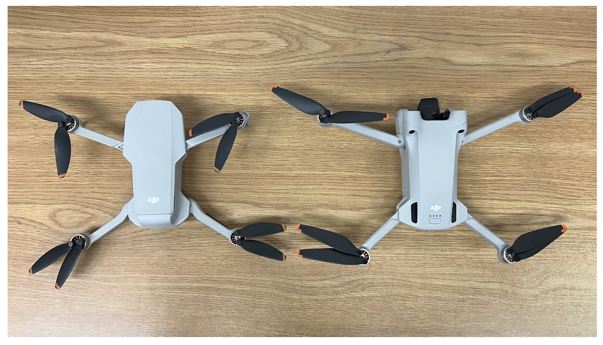
An important aspect of wind turbine fault analysis is the investigation of dataset creation and the inspection method. Due to the height and remote nature of wind turbine farms, drones are often deployed to gather sufficient data for training deep learning models. However, through drone path-planning research, drones possess the capability of autonomously flying to wind turbines to capture images of the blades. In this area, smaller-scale experiments have been conducted to verify the concept and implement the algorithms in a controlled environment [35,36].
Recent works have used drone inspection and machine learning to analyze wind turbine blade damage. Previous approaches to blade fault detection include the use of residual and wavelet-based neural networks, feature detection using Haar-like features, SVM with fuzzy logic, etc. [37,38,39]. In China, an alternate approach to the problem was recently employed via Unmanned Aerial Vehicles (UAVs) to first capture images of wind turbine blades and then use a cascading classifier algorithm to identify and locate wind turbine blade cracks [34,40]. ResNet-50, pretrained with ImageNet weights and with custom fully connected top layers, has been used in other works to provide high test precision and recall on identifying small blade chips and cracks [41].
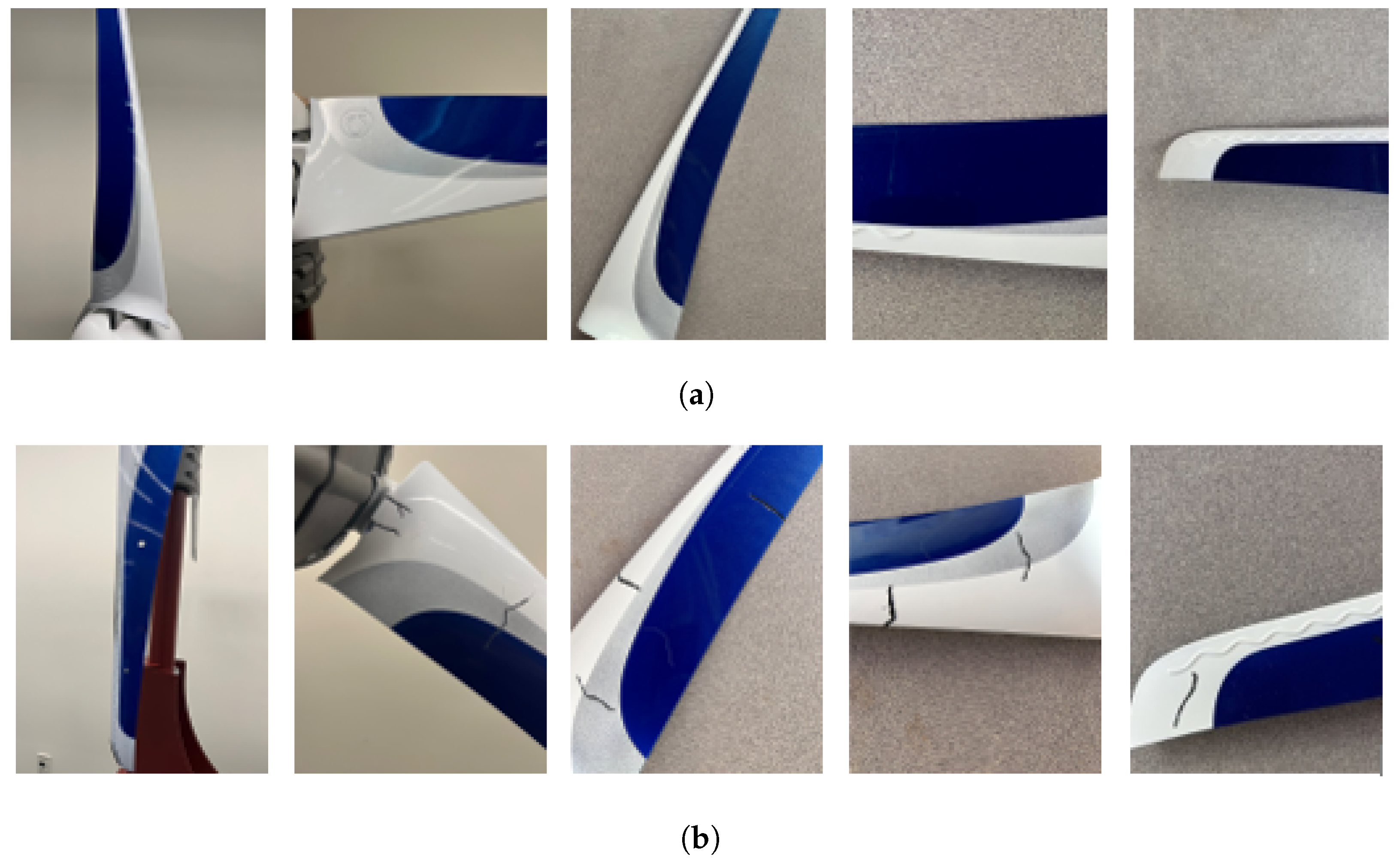
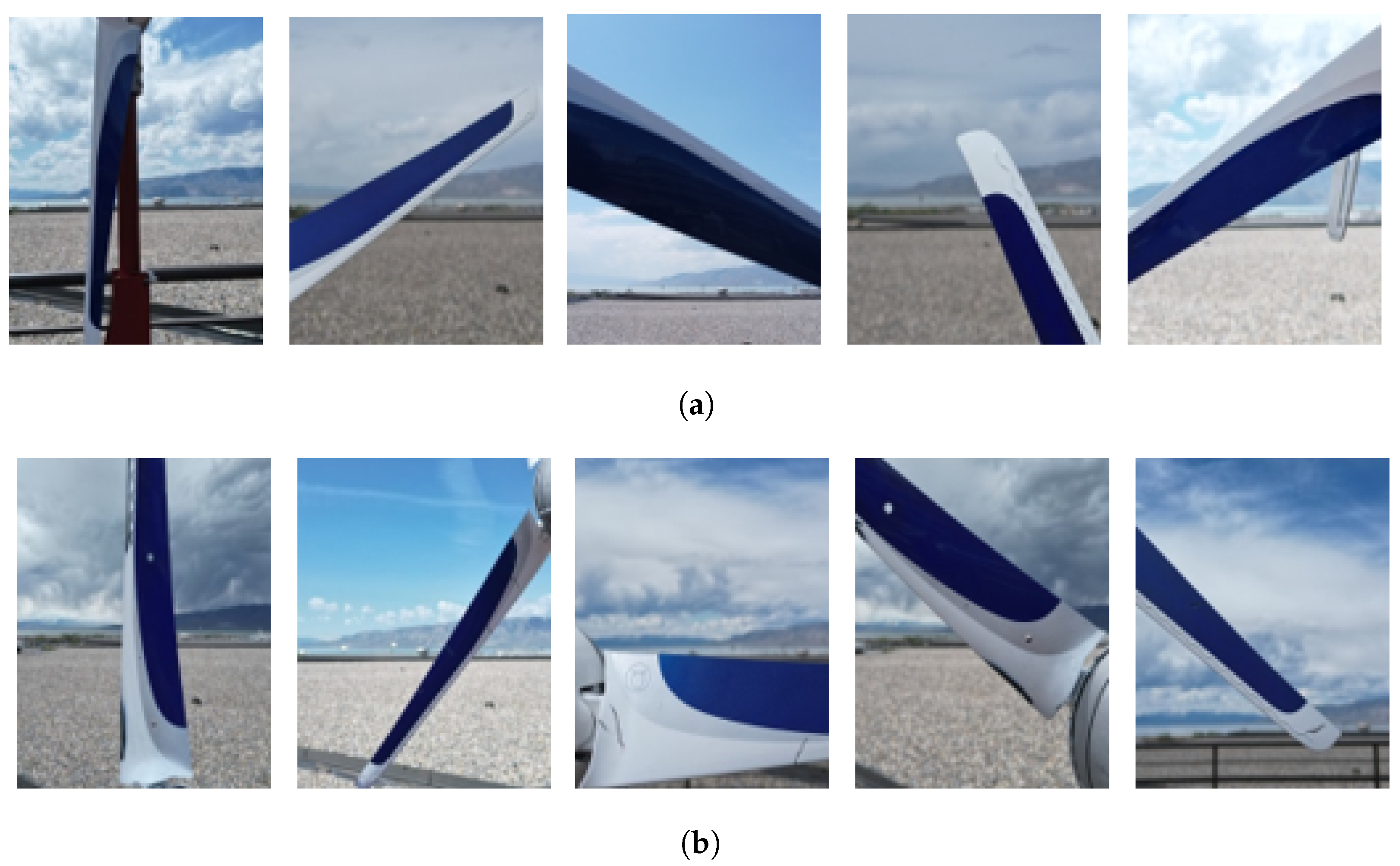
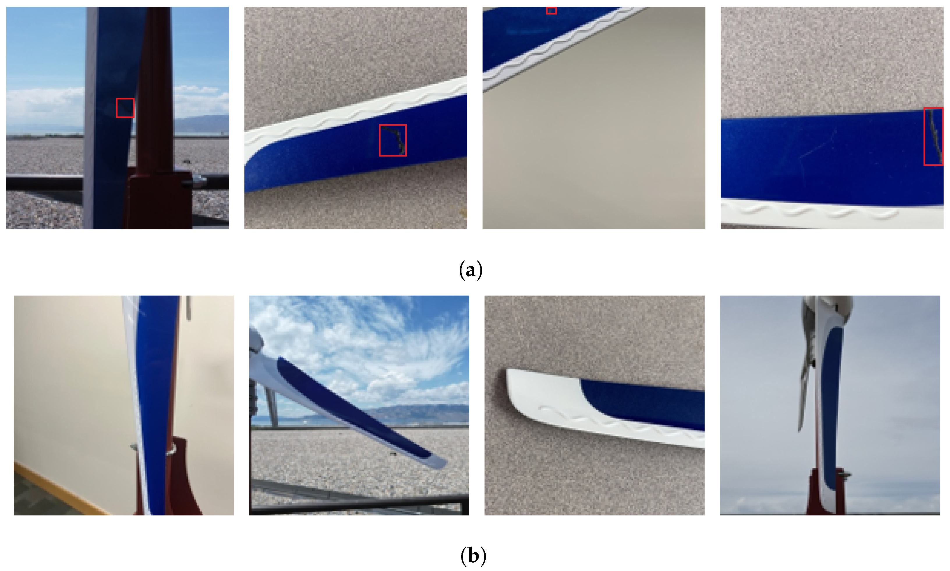
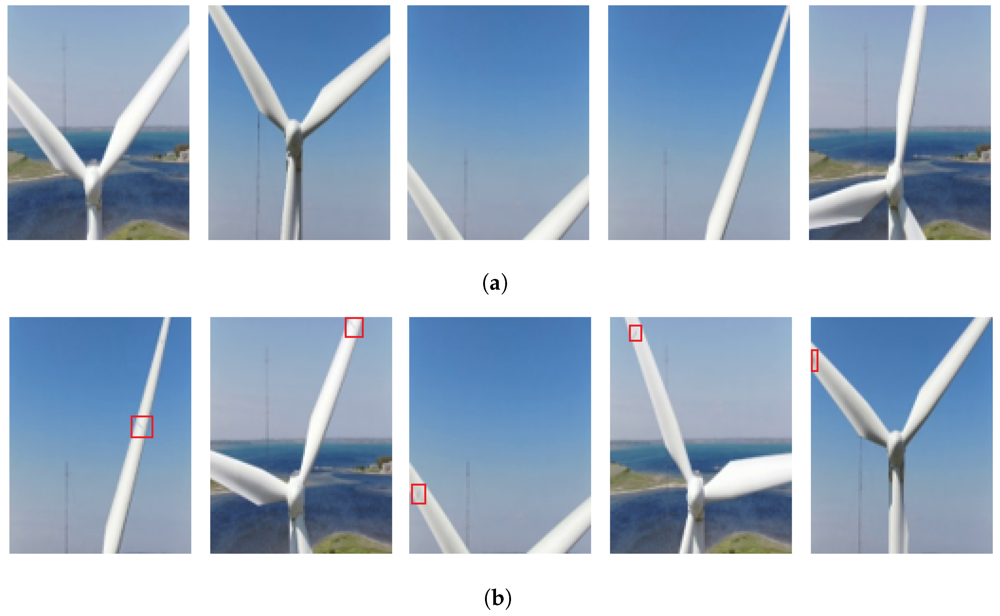
This research investigates the use of CNNs for the detection of faults within small wind turbine blade images. The CNN models are trained on a newly created dataset containing images of small wind turbine blades. This unique dataset contains multicolored images of wind turbine blades of the Primus AirMax turbine, rather than just white, monochromatic blades, and the damage on these blades includes cracks, holes, and edge erosion. The additional faults in the created dataset used here are not included in other datasets utilized in other works in this area.
The main contributions of this research include the following:
  • The creation of a novel fault identification dataset named Combined Aerial and Indoor Small Wind Turbine Blade (CAI-SWTB), utilizing images of healthy and damaged blades on a Primus AirMax wind turbine with a power output range of 0– 0.425 kW.
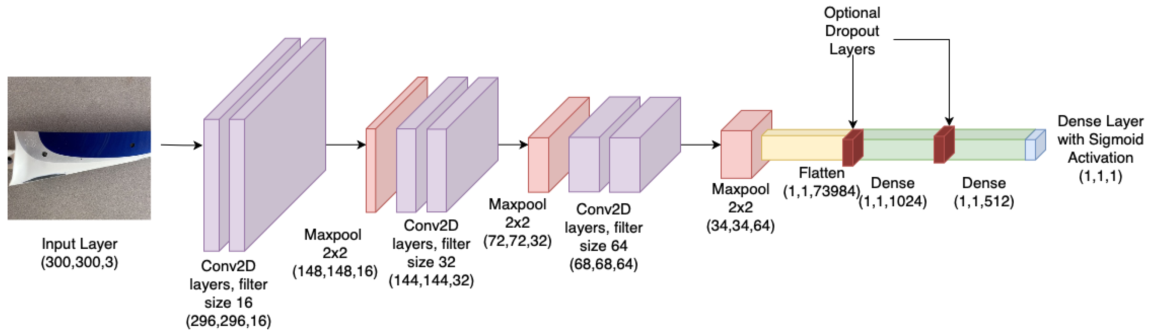
  • The development, training, and testing of a new custom CNN architecture and transfer learning models, making use of pretrained backbone networks to detect anomalies and damage on small wind turbine blades.
  • The investigation of transfer learning techniques in wind turbine fault classification.
  • Hyperparameter tuning and testing for optimal performance on the newly created CAI-SWTB dataset.
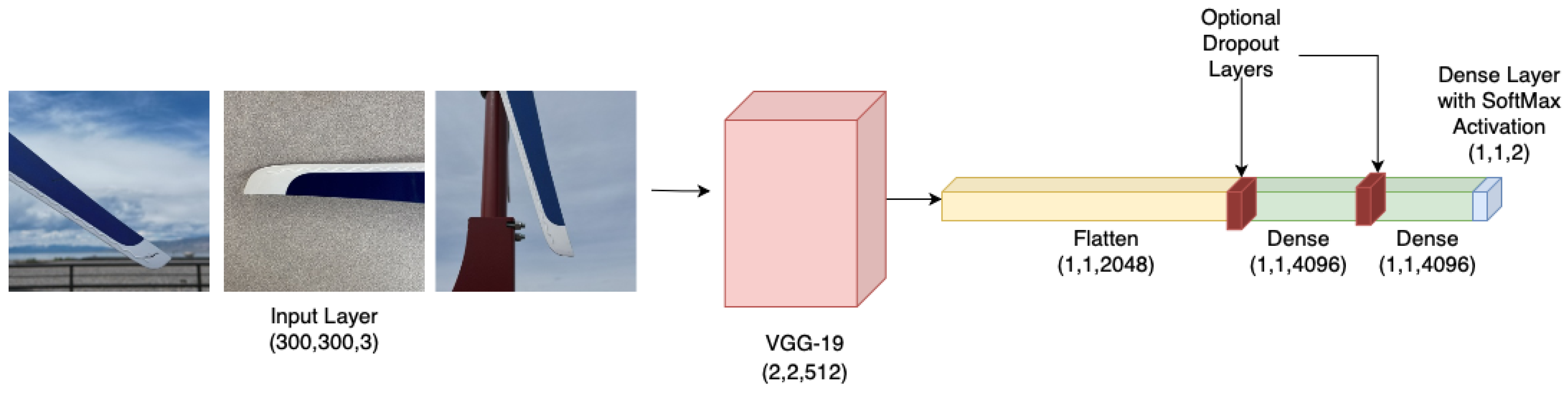
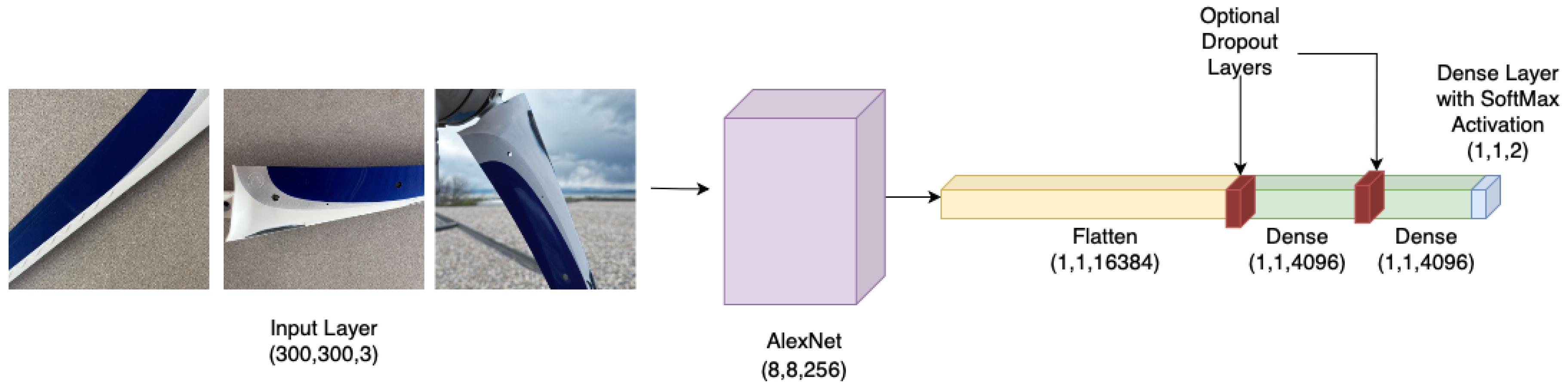
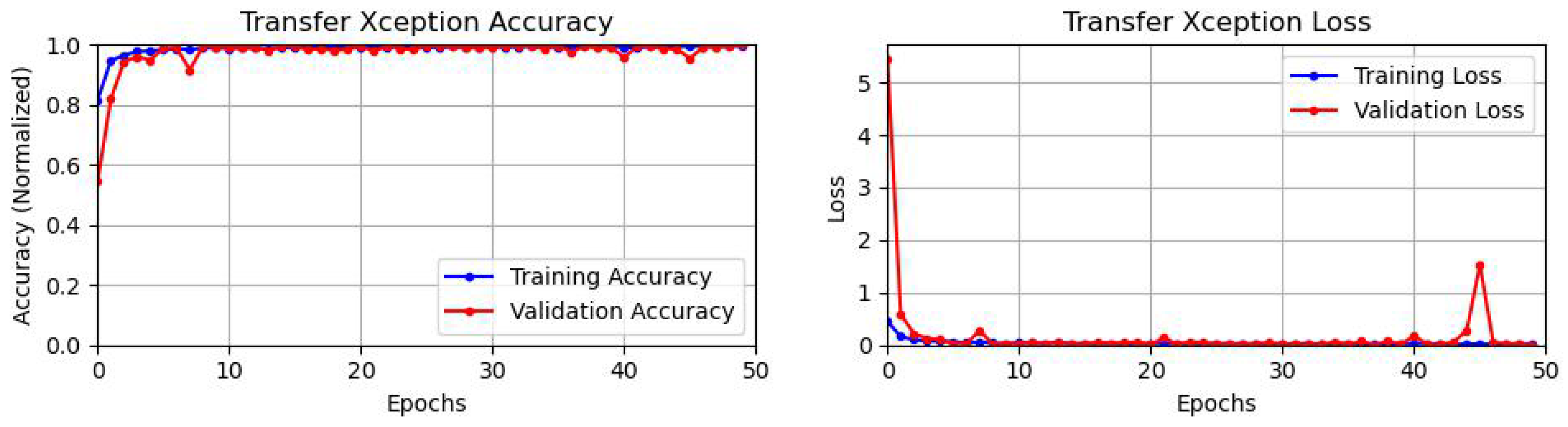
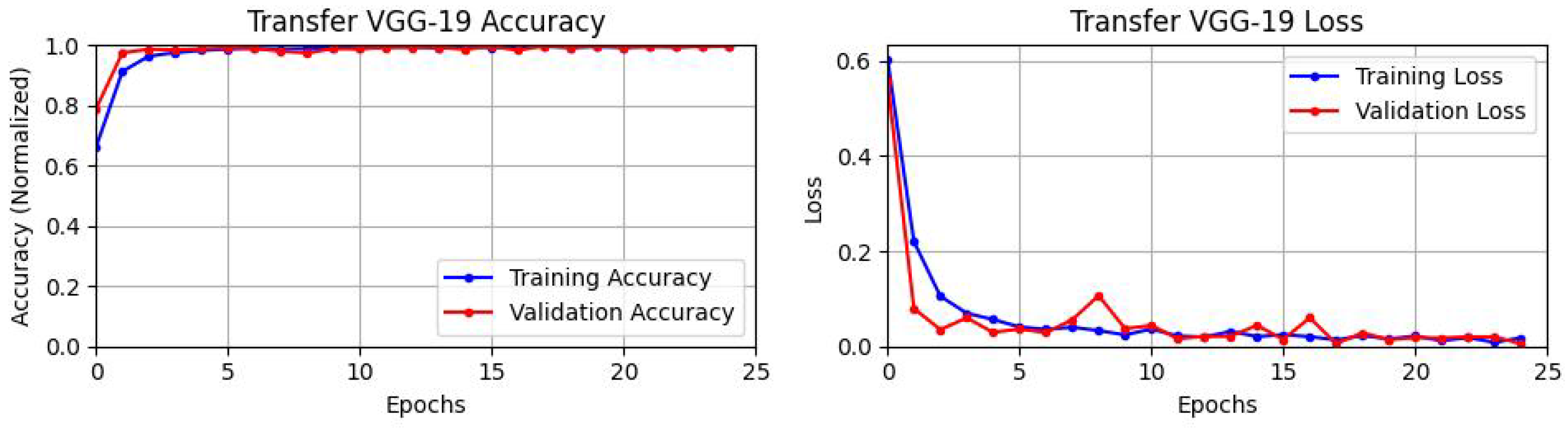
  • A comparison of Xception, ResNet-50, VGG-19, and AlexNet against the custom architecture and proposed transfer learning methods.
The rest of this paper is organized as follows. Section 2 discusses the deep learning architectures deployed in our research of anomaly detection. The newly created dataset, Combined Aerial and Indoor Small Wind Turbine Blade CAI-SWTB, is detailed in Section 4, followed by simulations, results, and a discussion. Finally, some conclusions and suggestions for future work are presented in Section 5.

2. Deep Learning Architecture Overview

The architectures discussed in this research are derived from CNNs. CNNs are a type of neural network that uses kernels of differing sizes to determine the next layer’s connection. This reduces the number of computations compared to a traditional fully connected neural network, vital for large image classification. These kernels are comprised of weights and biases that can be trained through backpropagation to produce regional feature-extracting capabilities. A typical architecture of a CNN is illustrated in Figure 1. Here, the convolutional kernels and final fully connected layer are depicted alongside the pooling layers, which provide downsampling while maintaining important features. A further detailed explanation of CNN architectures and their creation can be found in [42,43].

2.1. Visual Geometry Group-19

Visual Geometry Group (VGG) is a CNN architecture developed in 2014 by Karen Simonyan and Andrew Zisserman [44]. This architecture includes a pattern of convolution and max-pooling blocks followed by fully connected layers at the end of the model. The number after VGG denotes the number of trainable weighted layers in that specific variant. VGG-19 has a total of 16 convolutional layers, 4 max-pool layers, and 3 fully connected layers that are trainable. Figure 2 shows the outputs from each layer.

2.2. Custom Convolutional Neural Network

The second model that is proposed here is a custom CNN network. This architecture replicates the properties of VGG-19. It contains six convolutional layers, three max-pool layers, a dropout layer, varying dense layers, activation functions, and optimization functions. The size of the input image is 300 × 300. Each convolutional layer uses a ReLU activation function and a 3 × 3 kernel size. The first two 2D convolutional layers use a filter size of 16, the next two use a filter size of 32, and the last two use a filter size of 64. This filter is chosen to be smaller in the first convolutional layers so the model can detect simpler/larger features. Once those are detected, the filter size is increased so the model can detect the smaller or more complex features in the images. Each max-pool layer has a size of 2 × 2. The learning rate for this architecture is set to 0.001 to reduce the number of parameters being tuned. The model is illustrated in Figure 3, which depicts how the shape and size of the data change as they progress through each layer.

2.3. Xception

Xception, also known as Extreme Inception, was developed by Google in 2017 [45]. Xception takes the properties of its predecessor, the Inception model, and enhances them significantly, utilizing features such as depthwise separable convolutional layers and skip connections. Depthwise separable convolution reduces processing time and accounts for most input features by first performing convolution on each of the three color channels in an RGB image separately and then concatenating each output [45]. Within each convolutional layer, kernels of varying sizes are used to perform convolution, each followed by a 1 × 1 pointwise convolution. Then, each result is combined through filter concatenation. Using a variety of kernel sizes allows for more features to be extracted from each input. Overall, Xception contains a total of 74 separable convolutional, activation, pooling, and fully connected layers.

2.4. AlexNet

AlexNet was developed by Alex Krizhevsky, Ilya Sutskever, and Geoffrey Hinton in 2012 to participate in the ImageNet competition [46]. The architecture takes a unique approach to CNNs by using unconventional filters and kernel sizes for the convolutional layers. Figure 4 shows the output of each layer in the architecture. AlexNet was chosen to assess how the dataset would perform on an earlier convolutional neural network architecture.

2.5. ResNet-50

ResNet-50 is the 50-layer version of the residual CNNs proposed by He et al. [47]. This family of networks is characterized by skip and residual connections. Skip connections were created to correct the issue of backpropagation loss in deep networks by providing a path for backpropagation to reach earlier layers and eliminate the vanishing gradient problem. Solving this gradient problem allows for more convolutional layers to be processed with less computational time per layer. Residual connections are also used, which allows for the residual function of the input layer to be incorporated.

2.6. Transfer Learning

Transfer learning (TL) is the process of using pretrained neuron weights from one model and applying them to another model to be trained for a different purpose [48]. These pretrained weights are used so that a model has a reasonable starting point for training, rather than starting from scratch with default neuron weights.
One transfer learning approach is to freeze the pretrained feature extraction layers and then only train the remaining top dense layers on the desired dataset. The idea is that the frozen layers will already be trained for general image classification. Thus, only the top layers need to be fine-tuned for the specific purposes of the transfer learning model. Training only the top layers significantly reduces training time. An alternative approach is to use the pretrained layers as a base and further train all layers of the model, including the pretrained layers, on the new desired dataset. Since in this approach, every layer is updated, it takes more time compared to the first approach to reach high test and validation accuracies, but it is still faster than training the model completely from scratch.
For this research, the pretrained Keras ImageNet weights for VGG-19, Xception, and ResNet-50 were applied to each of these architectures. The pretrained layer-freezing approach was implemented for all three models. The second approach, where the pretrained layers were not frozen, was also implemented with various top layers. Each model benefited from the unfrozen pretrained layer approach, which achieved better accuracy and quicker convergence compared to the frozen-only approach.

3. Simulation Results and Discussion

In this section, the simulation environment for the training and comparison of each model is described. The newly created dataset utilized for this research is introduced in detail, and the evaluation results are discussed. Here, the created dataset simulates the damage that can occur in large-scale wind turbine blades, including cracks, holes, and erosion, which are commonly caused by environmental factors such as storm conditions, freezing and thawing, air pollutants, etc. [49]. Lightning strikes can also cause immense damage to wind turbines, leading to holes and scorching of the material [49,50]. Edge erosion, especially that of the leading edge, can cause decreases in energy production performance and a reduction in blade service expectancy [51]. Finally, a large-scale wind turbine dataset is examined to further evaluate the performance of these models in this application [52].

3.1. Hardware Specifications

Four computers were used to run the simulations. The first computer consists of GPU hardware obtained from Google Colaboratory, containing an Intel Xeon CPU and an NVIDIA Tesla T4 GPU. The second computer uses an Intel I9-11900k CPU and an NVIDIA 3070 with 10 GB of VRAM. The third computer contains an Intel I7-12700k CPU paired with an NVIDIA 4070 GPU with 12 GB of VRAM. The fourth computer accessed Center for High-Performance Computing (CHPC) resources from the University of Utah, which utilizes varying GPUs.

3.2. Hyperparameter Tuning

Hyperparameter tuning is the process of changing model parameters to find a combination for optimal performance. This includes the optimization algorithm, number of epochs, dropout layer rates, and optimizer learning rates. Here, hyperparameter tuning was implemented using custom functions during the building of each architecture to incorporate the parameters required for the current model. The parameters considered in our simulations included the epochs, dropout rate, activation function, optimization algorithm, batch size, pooling layer, and learning rate. In each simulation, the loss function was consistent with binary cross-entropy, as was the image size and dataset split, as noted in Table 1. Through exhaustive searching of these different parameters, optimal configurations were found.

3.3. Combined Aerial and Indoor Small Wind Turbine Blade Dataset Results

Due to the unavailability of sufficient public images of damaged commercial-grade large-scale turbine blades, a Primus Air Max wind turbine was deployed to create the small wind turbine dataset used in this research. A total of six blades were used to create a set of healthy blades and a set of faulty blades for the purpose of dataset generation. The faults inflicted on the blades were intended to simulate those that affect commercial-grade turbines, such as cracks, holes, and edge erosion. These anomalies were applied to both the front and back surfaces of the blade. Following the creation of these simulated faults, images were collected to create the dataset.
Simulating a traditional snapshot of damage taken during human inspection, images of the newly created faulty and healthy Primus AirMax wind turbine blades were taken using a smartphone within an indoor environment. In total, 4000 RGB images were collected within this environment, containing a 50% faulty and 50% healthy distribution. Figure 5 illustrates a sample of the images collected in this environment. To introduce more realistic environmental features into our dataset, the small wind turbine was also placed outside on a balcony, and images were taken utilizing DJI Mini 3 Pro and Mini SE drones, as illustrated in Figure 6. This allowed for a more diverse set of features to be present in the dataset, including environmental variables such as clouds and sunlight. Samples from the dataset of these outdoor images are shown in Figure 7. A total of 2000 RGB aerial images were captured, with the fixed distribution of faults being 50%.
By merging both sets, the final dataset comprised 4000 indoor and 2000 outdoor images, yielding a cumulative total of 6000 images, each with a size of 300 × 300 × 3. These images were then divided into faulty or healthy classes to enable binary classification. The name of this dataset is the Combined Aerial and Indoor Small Wind Turbine Blade (CAI-SWTB) dataset. These images were split into 70% for training, 20% for testing, and 10% for validation. The total number of images in each class is detailed in Table 1. To access the created dataset, please see the Data Availability Statement on page 18.
Here, each model outlined in Section 2 is trained and tuned on the CAI-SWTB dataset, followed by a comparison and discussion. To investigate model performance in each environment present in the dataset, the evaluation is performed in three stages. First, each model is trained and evaluated on the full dataset containing indoor and outdoor images. This is followed by an evaluation and discussion of the performance on the indoor test images. Finally, the results of the aerial images are discussed. The metrics utilized in our comparisons include accuracy, precision, recall, and F1-score. These values are obtained by having the model make predictions on each test image in the dataset and comparing them to the actual labels using scikit-learn’s metrics model. In the subsections that follow, the augmentation scheme utilized in the training is discussed, leading to the analysis of the performance on the evaluation set in each respective environment.

3.3.1. Preprocessing and Image Augmentation

To assist with model training and convergence, image augmentation was deployed to increase the number of unique images seen by a model. This process applied different filters to the dataset, such as tilting, zooming, and shearing. Before the images were augmented, they were first normalized by dividing the pixel values by 255. Image augmentation was implemented using Keras’s preprocessing Image Data Generator. Table 2 shows the utilized parameters, including random variations in zoom, shear, rotation, and flipping. Here, the values were chosen conservatively to maintain the fault features of the images. While the number of images in the training set remained fixed, the number of unique image variations seen by the model increased.

3.3.2. Results on the Combined Indoor and Outdoor Images from CAI-SWTB: Full Dataset

The tuning of each model was conducted according to the hyperparameter search space discussed in Section 3.2, with the corresponding results of the tuning illustrated in Table 3. Following training on the CAI-SWTB dataset using the best-found hyperparameters, each model was evaluated on the unseen test set. The performance of each model is presented in Table 4. In this table, it is shown that the transfer learning technique provided consistent improvements over the base variants for each model. The TL-Xception model achieved the highest accuracy of 99.92%. This was followed by TL-VGG-19 and Base Xception, with accuracies of 99.83% and 99.33%, respectively. The custom CNN created in this research achieved an accuracy of 96.67% which is notable considering it is 12 layers deep compared to the larger models of Xception with 71 layers and ResNet-50 with 50 layers.
To further visualize the performance of each model during training, their accuracy and loss values were plotted against the epochs, as shown in Figure 8, Figure 9, Figure 10, Figure 11, Figure 12, Figure 13, Figure 14 and Figure 15. The transfer learning variants achieved the highest accuracy at earlier epochs (see Figure 8) compared to the base architectures. This is due to the leveraged weights providing a better starting point for model convergence on this dataset. Subsequently, each transfer learning model also achieved minimized loss in fewer epochs. The custom CNN model required more epochs to converge (see Figure 14); however, it was similar to the base VGG-19 and AlexNet (see Figure 13 and Figure 15) due to the similar layer size and architectural features. Consequently, the loss value also followed this pattern.
Model size and layer count are important features of CNNs, as smaller models provide quicker inference and training time. However, lower layer counts can reduce the feature extraction capability of the model, leading to lower accuracy. AlexNet contains only 12 layers, including the feature extraction and fully connected layers. Subsequently, AlexNet achieved the worst accuracy among the base architectures with a test accuracy of 95.08%. This was followed by the custom CNN, which achieved an accuracy of 96.67% and had a similar layer count to AlexNet. The trend in our data correlates with the deeper architectures by layer count, achieving higher accuracy in the classification of wind turbine faults. The model with the highest accuracy in our research, TL-Xception, contains 71 layers and is the largest in our research.
In the investigation of commonly miscategorized images, as shown in Figure 16, it was found that the reflective surface of the blade was the primary cause of incorrect categorization. The reflections of the indoor lighting can be seen in Figure 16b and appear similar to the simulated cracks on the blade in shape, size, and placement. This led to an increase in false positives, where the model prediction was faulty and the true label was healthy, in the majority of model predictions. Figure 16a depicts common false negatives, which were predicted healthy when the true label was faulty, from the top-performing architectures. Similar to the indoor reflections, the sun reflections in the outdoor images obscured the faults in a manner that led the architectures to perceive them as healthy. Another factor included dark cracks, which blended in with the dark-blue portion of the turbine blade. The theorized cause for this is the difference in the lighting conditions for the indoor vs. outdoor images. When the blade was not illuminated, the cracks became difficult to discern in the blue region of the blade. This is an important factor in the adoption of the proposed fault analysis method and can be solved in the following ways. Most wind turbine blades are a solid white color rather than the multicolored one in our dataset, so images like the ones shown in Figure 16 would be less often mislabeled as healthy in commercial applications.

3.3.3. Results on Indoor Images from CAI-SWTB Dataset

For further analysis of the trained models, here, we study how they performed on just the indoor portion of the dataset. It is important to note that these models were trained on the combination of indoor and outdoor images together prior to being evaluated on the test data from the indoor subsection, totaling 800 images, as seen in Table 1. The model performance on the indoor test images is shown in Table 5. The results show that the TL-Xception model exhibited the highest accuracy, achieving 100% accuracy on the indoor image test set. This was followed by TL-VGG-19 and the base Xception, with accuracies of 99.88 % and 99.5%, respectively. The proposed custom CNN also exhibited notable performance on this set of data, achieving 98.62% accuracy. Each model achieved above 90% accuracy on this subset of data, showing promise for synthesizing faults.

3.3.4. Results on Outdoor Aerial Images from CAI-SWTB Dataset

Following the evaluation of the indoor test data, the impact of the environmental features introduced in the outdoor aerial image portion of the dataset was investigated. The total test allocation of the aerial images included 200 healthy and 200 faulty images. The performance on the aerial image subset of the test data is illustrated in Table 6. Here, it can be seen that the highest accuracy of 99.75% was achieved by both TL-Xception and TL-VGG-19. This was followed by the base Xception and base ResNet-50, both achieving 99% accuracy on this set. The custom CNN’s performance dropped on the outdoor data; however, it still achieved 95% accuracy. Overall, each model achieved above 90% accuracy, showing a promising trend in the ability to determine faults in the domain of wind turbine blades.

3.4. Performance on Large-Scale Wind Turbine Dataset

To further compare model performance and gauge performance on large-scale turbines, the Drone-Based Optical and Thermal Videos of Rotor Blades Taken in Normal Wind Turbine Operation dataset was utilized [53]. This dataset contains images of faulty and healthy turbine blades in a variety of formats, including thermal, RGB, and low light, taken with DJI drones. For a fair comparison between our dataset and this dataset, the daytime RGB images from this dataset were selected for analysis. To preserve model input size and overall parameters, the images were also downscaled from their original size of 853 × 480 to 300 × 300 , allowing the data to match the size of the data in the CAI-SWTB dataset. Additionally, to address the imbalance in representation between faulty and healthy turbine blades in this dataset, a random selection was made to ensure an equal split of faulty and healthy images. This resulted in a total of 516 images, with 258 images in each class, representing both faulty and healthy turbine blades. These images were then randomly split into training, validation, and test sets, using the same split used for the CAI-SWTB dataset: 70% training, 20% testing, and 10% validation. These split totals are shown in Table 7. Samples from this dataset are shown in Figure 17, with the healthy blades shown in Figure 17a, and the faulty blades shown in Figure 17b. Here, the positions of the faults are highlighted with a box. The faults included in this dataset consist of cracks at various positions in the blade lengths, captured through drone aerial imagery.
To ensure a fair comparison, each model underwent hyperparameter tuning on this new dataset, consistent with the simulations conducted on the CAI-SWTB dataset, using the search space defined in Section 3.2. The resulting tuned hyperparameters are illustrated in Table 8. Since many of the cracks in these images appear near the image border, the image augmentation parameters for the models using this dataset had to be modified for the augmented images to ensure the existence of blade cracks. For example, if an image contained a crack near the edge and the image was stretched, zoomed, and/or rotated, the crack in the image would likely be moved out of the image window. However, horizontal flipping maintained the image contents while providing more variations to help reduce overfitting and result in better generalization. Thus, in order to maintain the intended features of the dataset, the augmentation parameters described in Table 9 were applied.
The evaluation of the performance of the investigated models on this dataset is illustrated in Table 10 and Figure 18, Figure 19, Figure 20, Figure 21 and Figure 22. Here, the best accuracy achieved was 100% by the transfer learning-based Xception model. This was followed by the other two transfer learning variants in our study, (TL)-VGG-19 and (TL)-ResNet50, achieving accuracies of 98.08% and 93.27%, respectively. Among the non-transfer learning models, the custom CNN achieved the highest accuracy of 80.77%. Here, the smaller dataset and limited features represented proved to be beneficial for the lower layer count. Similarly, AlexNet outperformed the larger non-transfer learning models, achieving 78.85% accuracy. The other models in our study, the base ResNet50, base Xception, and base VGG-19, were omitted due to poor performance on this dataset. The limited number of images and inability to apply image augmentation caused these deeper models to overfit quickly and fail to generalize the fault features. This overfitting trend can also be seen in the loss vs. epoch plots for the custom CNN (see Figure 21) and AlexNet (see Figure 22). Here, the validation loss became divergent while the training loss continued a downward trend, indicating poor generalization on unseen data. To address this issue, more images would be required to bolster the image count for the dataset while introducing variance to the representation presented to the model. However, with the inherent challenges of this limited dataset, the performance of the transfer learning architectures showed promising results. Leveraging pretrained model weights with additional fine-tuning allowed for convergence and provided exceptional accuracy on this dataset.

4. Conclusions

This study conducted binary fault classification of small wind turbine blades using a newly created dataset of 6000 RGB images. The created dataset included simulated faults of cracks, holes, and edge erosion in varying environments. A custom convolutional neural network was investigated, along with four existing architectures. Leveraging these four architectures as the feature extraction backbone, three transfer learning approaches were also developed and compared. Through an exhaustive search of hyperparameters, an optimal set was found for each architecture on the created CAI-SWTB dataset, providing the best accuracy. Here, it was shown that the proposed transfer learning Xception architecture outperformed other architectures, achieving 99.92% accuracy. This was followed by the transfer learning-based VGG-19 and base Xception models, with accuracies of 99.83% and 99.33%, respectively. An additional study, utilizing a dataset containing faulty and healthy large-scale wind turbine blades, was also conducted to compare model performance. While limited in scope and size, this dataset allowed for the testing of the investigated models on large-scale commercial turbines. This dataset was created using an autonomous drone. Our results on this limited data showed that the transfer learning-based Xception model achieved the highest accuracy of 100%.

5. Future Work

Our results show that deep learning is a promising technology for classifying and identifying faults on wind turbine blades for preventative maintenance. However, further study is required to improve performance and expand the information extracted from these images. Our future research will include the investigation of fault localization and fault size estimation, utilizing object detection architectures and feature detection techniques to allow more detailed information to be provided to maintenance engineers. Furthermore, this work mostly focused on stationary wind turbines, which requires halting the turbine, leading to losses in energy production and output. To address this concern, our future work will also explore de-blurring the aerial images taken of rotating blades. Thus, inspections can be performed on turbines in active operation with moderate wind speed. Additionally, to address the inspection needs of large-scale commercial turbines and their inherent environmental condition challenges, the deployment of larger industrial-grade drones will be utilized. In this case, our future work will focus on autonomous inspections, utilizing vision-based path planning, and inspections using a DJI Matrice 300 RTK. This drone provides stability in wind speeds of up to 15 m/s, allowing usage in these high-wind environments.

Author Contributions

Conceptualization, M.S.; methodology, B.A., E.N. and M.D.; software, B.A., E.N. and M.D.; validation, B.A., E.N. and M.D.; formal analysis, B.A., E.N., M.D., M.S. and T.K.M.; investigation, B.A., E.N. and M.D.; resources, M.S. and M.A.S.M.; data curation, M.S. and E.N.; writing—original draft preparation, B.A., E.N. and M.D.; writing—review and editing, B.A., E.N., M.D., M.S., T.K.M. and M.A.S.M.; visualization, B.A., E.N. and M.D.; supervision, M.S. and T.K.M.; project administration, M.S.; funding acquisition, M.S. and M.A.S.M. All authors have read and agreed to the published version of the manuscript.

Funding

This research was funded by the Office of the Commissioner of Utah System of Higher Education (USHE)—Deep Technology Initiative Grant 20210016UT.

Data Availability Statement

The created Combined Indoor and Outdoor Small Wind Turbine (CAI-SWTB) dataset can be accessed at the following link: https://www.kaggle.com/datasets/mohammadshekaramiz/small-wind-turbine-blade-dataset-cai-swtb (accessed on 1 February 2024).

Acknowledgments

The authors would like to thank UVU students Vicky Odhiambo, Joshua Zander, and Jeremiah Engel for their contributions to the creation of the CAI-SWTB dataset.

Conflicts of Interest

The authors declare no conflicts of interest.

Abbreviations

The following abbreviations are used in this manuscript:
AFActivation Function
CAI-SWTB datasetCombined Aerial and Indoor Small Wind Turbine Blade dataset
CHPCCenter for High-Performance Computing
CNNConvolutional Neural Network
EACEnhanced Asymmetric Convolutional
LRLearning Rate
PCAPrincipal Component Analysis
ResNetResidual Network
SCADASupervisory Control and Data Acquisition
SVMSupport Vector Machine
TLTransfer Learning
UAVUnmanned Ariel Vehicle
VGGVisual Geometry Group
XceptionExtreme Inception
YOLOYou Only Look Once

References

  1. Samour, A.; Mehmood, U.; Radulescu, M.; Budu, R.A.; Nitu, R.M. Examining the role of renewable energy, technological innovation, and the insurance market in environmental sustainability in the United States: A step toward COP26 targets. Energies 2023, 16, 6138. [Google Scholar] [CrossRef]
  2. Energy Facts Explained—Consumption and Production—U.S. Energy Information Administration (EIA). Available online: https://www.eia.gov/energyexplained/us-energy-facts/ (accessed on 15 January 2023).
  3. Xu, X.; Wei, Z.; Ji, Q.; Wang, C.; Gao, G. Global renewable energy development: Influencing factors, trend predictions and countermeasures. Resour. Policy 2019, 63, 101470. [Google Scholar] [CrossRef]
  4. Kim, S.K.; Park, S. Impacts of renewable energy on climate vulnerability: A global perspective for energy transition in a climate adaptation framework. Sci. Total Environ. 2023, 859, 160175. [Google Scholar] [CrossRef]
  5. Hawkins Kreps, B. The rising costs of fossil-fuel extraction: An energy crisis that will not go away. Am. J. Econ. Sociol. 2020, 79, 695–717. [Google Scholar] [CrossRef]
  6. Fernández, L. Share of Electricity Generation from Wind Energy Sources Worldwide from 2010 to 2022. 2023. Available online: https://www.statista.com/statistics/1302053/global-wind-energy-share-electricity-mix/ (accessed on 18 August 2023).
  7. International Energy Agency. Tracking Wind Electricity. Available online: https://www.iea.org/energy-system/renewables/wind (accessed on 18 August 2023).
  8. Zou, L.; Cheng, H.; Sun, Q. Surface damage identification of wind turbine blade based on improved lightweight asymmetric convolutional neural network. Appl. Sci. 2023, 13, 6330. [Google Scholar] [CrossRef]
  9. Katsaprakakis, D.A.; Papadakis, N.; Ntintakis, I. A comprehensive analysis of wind turbine blade damage. Energies 2021, 14, 5974. [Google Scholar] [CrossRef]
  10. U.S. Energy Information Administration. Wind Turbine Heights and Capacities Have Increased over the Past Decade. 2017. Available online: https://www.eia.gov/todayinenergy/detail.php?id=33912 (accessed on 18 August 2023).
  11. Scheu, M.; Matha, D.; Schwarzkopf, M.A.; Kolios, A. Human exposure to motion during maintenance on floating offshore wind turbines. Ocean Eng. 2018, 165, 293–306. [Google Scholar] [CrossRef]
  12. Dimitrova, M.; Aminzadeh, A.; Meiabadi, M.S.; Sattarpanah Karganroudi, S.; Taheri, H.; Ibrahim, H. A survey on non-destructive smart inspection of wind turbine blades based on industry 4.0 strategy. Appl. Mech. 2022, 3, 1299–1326. [Google Scholar] [CrossRef]
  13. Liu, Y.; Wu, Z.; Wang, X. Research on fault diagnosis of wind turbine based on SCADA data. IEEE Access 2020, 8, 185557–185569. [Google Scholar] [CrossRef]
  14. Waqas Khan, P.; Byun, Y.C. Multi-fault detection and classification of wind turbines using stacking classifier. Sensors 2022, 22, 6955. [Google Scholar]
  15. Ng, E.Y.K.; Lim, J.T. Machine learning on fault diagnosis in wind turbines. Fluids 2022, 7, 371. [Google Scholar] [CrossRef]
  16. Cui, Y.; Bangalore, P.; Tjernberg, L.B. An Anomaly Detection Approach Based on Machine Learning and SCADA Data for Condition Monitoring of Wind Turbines. In Proceedings of the IEEE International Conference on Probabilistic Methods Applied to Power Systems (PMAPS), Boise, ID, USA, 24–28 June 2018; pp. 1–6. [Google Scholar]
  17. Velandia-Cardenas, C.; Vidal, Y.; Pozo, F. Wind turbine fault detection using highly imbalanced real SCADA data. Energies 2021, 14, 1728. [Google Scholar] [CrossRef]
  18. Ker, J.; Wang, L.; Rao, J.; Lim, T. Deep learning applications in medical image analysis. IEEE Access 2017, 6, 9375–9389. [Google Scholar] [CrossRef]
  19. Singh, P.; Singh, S.; Paprzycki, M. Optimised context encoder-based fusion approach with deep learning and nonlinear least square method for pan-sharpening. Int. J. Bio-Inspired Comput. 2024, 23, 53–67. [Google Scholar] [CrossRef]
  20. Cha, Y.J.; Choi, W.; Büyüköztürk, O. Deep learning-based crack damage detection using convolutional neural networks. Comput.-Aided Civ. Infrastruct. Eng. 2017, 32, 361–378. [Google Scholar] [CrossRef]
  21. Deng, L.; Li, J.; Huang, J.T.; Yao, K.; Yu, D.; Seide, F.; Seltzer, M.; Zweig, G.; He, X.; Williams, J.; et al. Recent advances in deep learning for speech research at Microsoft. In Proceedings of the 2013 IEEE International Conference on Acoustics, Speech and Signal Processing, Vancouver, BC, Canada, 26–31 May 2013; pp. 8604–8608. [Google Scholar]
  22. Rababaah, A.R. Machine learning comparative study for human posture classification using wearable sensors. Int. J. Comput. Sci. Math. 2023, 18, 54–69. [Google Scholar] [CrossRef]
  23. Liu, X.; Lu, S.; Ren, Y.; Wu, Z. Wind turbine anomaly detection based on SCADA data mining. Electronics 2020, 9, 751. [Google Scholar] [CrossRef]
  24. Xiao, C.; Liu, Z.; Zhang, T.; Zhang, X. Deep learning method for fault detection of wind turbine converter. Appl. Sci. 2021, 11, 1280. [Google Scholar] [CrossRef]
  25. Murgia, A.; Verbeke, R.; Tsiporkova, E.; Terzi, L.; Astolfi, D. Discussion on the suitability of SCADA-based condition monitoring for wind turbine fault diagnosis through temperature data analysis. Energies 2023, 16, 620. [Google Scholar] [CrossRef]
  26. Yu, Y.; Cao, H.; Liu, S.; Yang, S.; Bai, R. Image-Based Damage Recognition of Wind Turbine Blades. In Proceedings of the 2nd International Conference on Advanced Robotics and Mechatronics (ICARM), Hefei and Tai’an, China, 27 August 2017; pp. 161–166. [Google Scholar]
  27. Moreno, S.; Peña, M.; Toledo, A.; Treviño, R.; Ponce, H. A New Vision-based Method Using Deep Learning for Damage Inspection in Wind Turbine Blades. In Proceedings of the 15th International Conference on Electrical Engineering, Computing Science and Automatic Control (CCE), Mexico City, Mexico, 5 September 2018; pp. 1–5. [Google Scholar]
  28. Chen, Q.; Liu, Z.H.; Lv, M.Y. Attention Mechanism-based CNN for Surface Damage Detection of Wind Turbine Blades. In Proceedings of the 2022 International Conference on Machine Learning, Cloud Computing and Intelligent Mining (MLCCIM), Xiamen, China, 5 August 2022; pp. 313–319. [Google Scholar]
  29. Zou, L.; Cheng, H. Research on wind turbine blade surface damage identification based on improved convolution neural network. Appl. Sci. 2022, 12, 9338. [Google Scholar] [CrossRef]
  30. Memari, M.; Shekaramiz, M.; Masoum, M.A.; Seibi, A.C. Data Fusion and Ensemble Learning for Advanced Anomaly Detection Using Multi-Spectral RGB and Thermal Imaging of Small Wind Turbine Blades. Energies 2024, 17, 673. [Google Scholar] [CrossRef]
  31. Ran, X.; Zhang, S.; Wang, H.; Zhang, Z. An improved algorithm for wind turbine blade defect detection. IEEE Access 2022, 10, 122171–122181. [Google Scholar] [CrossRef]
  32. Zhang, C.; Yang, T.; Yang, J. Image recognition of wind turbine blade defects using attention-based MobileNetv1-YOLOv4 and transfer learning. Sensors 2022, 22, 6009. [Google Scholar] [CrossRef]
  33. Everingham, M.; Van Gool, L.; Williams, C.K.I.; Winn, J.; Zisserman, A. The Pascal visual object classes (VOC) challenge. Int. J. Comput. Vis. 2010, 88, 303–338. [Google Scholar] [CrossRef]
  34. Wang, L.; Zhang, Z.; Luo, X. A two-stage data-driven approach for image-based wind turbine blade crack inspections. IEEE/ASME Trans. Mechatron. 2019, 24, 1271–1281. [Google Scholar] [CrossRef]
  35. Pinney, B.; Stockett, B.; Shekaramiz, M.; Masoum, M.A.; Seibi, A.; Rodriguez, A. Exploration and Object Detection via Low-Cost Autonomous Drone. In Proceedings of the 2023 Intermountain Engineering, Technology and Computing (IETC), Provo, UT, USA, 12 May 2023; pp. 49–54. [Google Scholar]
  36. Pinney, B.; Duncan, S.; Shekaramiz, M.; Masoum, M.A. Drone Path Planning and Object Detection via QR Codes; A Surrogate Case Study for Wind Turbine Inspection. In Proceedings of the 2022 Intermountain Engineering, Technology and Computing (IETC), Orem, UT, USA, 13 May 2022; pp. 1–6. [Google Scholar]
  37. Seibi, C.; Ward, Z.; Masoum, M.A.; Shekaramiz, M. Locating and Extracting Wind Turbine Blade Cracks Using Haar-like Features and Clustering. In Proceedings of the 2022 Intermountain Engineering, Technology and Computing (IETC), Orem, UT, USA, 13 May 2022; pp. 1–5. [Google Scholar]
  38. N’Diaye, L.M.; Phillips, A.; Masoum, M.A.; Shekaramiz, M. Residual and Wavelet based Neural Network for the Fault Detection of Wind Turbine Blades. In Proceedings of the 2022 Intermountain Engineering, Technology and Computing (IETC), Orem, UT, USA, 13 May 2022; pp. 1–5. [Google Scholar]
  39. Seegmiller, C.; Chamberlain, B.; Miller, J.; Masoum, M.A.; Shekaramiz, M. Wind Turbine Fault Classification Using Support Vector Machines with Fuzzy Logic. In Proceedings of the 2022 Intermountain Engineering, Technology and Computing (IETC), Orem, UT, USA, 13 May 2022; pp. 1–5. [Google Scholar]
  40. Wang, L.; Zhang, Z. Automatic detection of wind turbine blade surface cracks based on UAV-taken images. IEEE Trans. Ind. Electron. 2017, 64, 7293–7303. [Google Scholar] [CrossRef]
  41. Iyer, A.; Nguyen, L.; Khushu, S. Learning to identify cracks on wind turbine blade surfaces using drone-based inspection images. arXiv 2022, arXiv:2207.11186. [Google Scholar]
  42. O’Shea, K.; Nash, R. An introduction to convolutional neural networks. arXiv 2015, arXiv:1511.08458. [Google Scholar]
  43. Albelwi, S.; Mahmood, A. A framework for designing the architectures of deep convolutional neural networks. Entropy 2017, 19, 242. [Google Scholar] [CrossRef]
  44. Simonyan, K.; Zisserman, A. Very deep convolutional networks for large-scale image recognition. arXiv 2015, arXiv:1409.1556. [Google Scholar]
  45. Chollet, F. Xception: Deep Learning with Depthwise Separable Convolutions. In Proceedings of the IEEE Conference on Computer Vision and Pattern Recognition (CVPR), Honolulu, HI, USA, 21–26 July 2017; pp. 1800–1807. [Google Scholar]
  46. Krizhevsky, A.; Sutskever, I.; Hinton, G.E. ImageNet Classification with Deep Convolutional Neural Networks. In Proceedings of the Advances in Neural Information Processing Systems, Lake Tahoe, CA, USA, 3–6 December 2012; Volume 25, pp. 1–9. [Google Scholar]
  47. He, K.; Zhang, X.; Ren, S.; Sun, J. Deep Residual Learning for Image Recognition. In Proceedings of the IEEE Conference on Computer Vision and Pattern Recognition (CVPR), Las Vegas, NV, USA, 27–30 June 2016; pp. 770–778. [Google Scholar]
  48. Mihalkova, L.; Mooney, R.J. Transfer Learning from Minimal Target Data by Mapping across Relational Domains. In Proceedings of the 21st International Joint Conference on Artificial Intelligence (IJCAI), Pasadena, CA, USA, 11–17 July 2009; Volume 9, pp. 1163–1168. [Google Scholar]
  49. Wang, W.; Xue, Y.; He, C.; Zhao, Y. Review of the typical damage and damage-detection methods of large wind turbine blades. Energies 2022, 15, 5672. [Google Scholar] [CrossRef]
  50. Garolera, A.C.; Madsen, S.F.; Nissim, M.; Myers, J.D.; Holboell, J. Lightning damage to wind turbine blades from wind farms in the US. IEEE Trans. Power Deliv. 2014, 31, 1043–1049. [Google Scholar] [CrossRef]
  51. Hasager, C.B.; Vejen, F.; Skrzypiński, W.R.; Tilg, A.M. Rain erosion load and its effect on leading-edge lifetime and potential of erosion-safe mode at wind turbines in the north sea and baltic sea. Energies 2021, 14, 1959. [Google Scholar] [CrossRef]
  52. Shihavuddin, A.; Chen, X.; Fedorov, V.; Nymark Christensen, A.; Andre Brogaard Riis, N.; Branner, K.; Bjorholm Dahl, A.; Reinhold Paulsen, R. Wind turbine surface damage detection by deep learning aided drone inspection analysis. Energies 2019, 12, 676. [Google Scholar] [CrossRef]
  53. Chen, X. Drone-based Optical and Thermal Videos of Rotor Blades Taken in Normal Wind Turbine Operation. IEEE Data Port 2023. [Google Scholar] [CrossRef]
Figure 1. Structure of a CNN [43].
Energies 17 00982 g001
Figure 2. VGG-19 model.
Energies 17 00982 g002
Figure 3. Custom CNN model.
Energies 17 00982 g003
Figure 4. AlexNet model.
Energies 17 00982 g004
Figure 5. Sample blade images from the created dataset (CAI-SWTB) taken in an indoor environment. (a) Sample images of healthy blades in an indoor environment. (b) Sample images of damaged (faulty) blades in an indoor environment.
Energies 17 00982 g005
Figure 6. Drones used for aerial imaging. From left to right: DJI Mini SE and DJI Mini 3 Pro.
Energies 17 00982 g006
Figure 7. Sample blade images from the created dataset (CAI-SWTB) taken in an outdoor environment. (a) Sample images of healthy blades in an outdoor environment. (b) Sample images of damaged (faulty) blades in an outdoor environment.
Energies 17 00982 g007
Figure 8. Best run results from the proposed transfer learning-based Xception, i.e., (TL)-Xception.
Energies 17 00982 g008
Figure 9. Best run results from the proposed transfer learning-based VGG-19, i.e., (TL)-VGG-19.
Energies 17 00982 g009
Figure 10. Best run results from base Xception.
Energies 17 00982 g010
Figure 11. Best run results from the proposed transfer learning-based ResNet-50, i.e., (TL)-ResNet-50.
Energies 17 00982 g011
Figure 12. Best run results from base ResNet-50.
Energies 17 00982 g012
Figure 13. Best run results from base VGG-19.
Energies 17 00982 g013
Figure 14. Best run results from custom CNN.
Energies 17 00982 g014
Figure 15. Best run results from base AlexNet.
Energies 17 00982 g015
Figure 16. Samples of commonly misclassified images using the implemented deep learning architectures. (a) Samples of false-negative images. Boxes indicate fault locations in the images. (b) Samples of false-positive images.
Energies 17 00982 g016
Figure 17. Sample blade images from the large-scale wind turbine dataset [53]. (a) Sample images of healthy blades on a large wind turbine. (b) Sample images of faulty blades on a large wind turbine. Boxes indicate fault locations in the images.
Energies 17 00982 g017
Figure 18. Best run results from the proposed transfer learning-based Xception, i.e., (TL)-Xception, on large-scale turbine data.
Energies 17 00982 g018
Figure 19. Best run results from the proposed transfer learning-based VGG-19, i.e., (TL)-VGG-19, on large-scale turbine data.
Energies 17 00982 g019
Figure 20. Best run results from the proposed transfer learning-based ResNet-50, i.e., (TL)-ResNet-50, on large-scale turbine data.
Energies 17 00982 g020
Figure 21. Best run results from custom CNN on large-scale turbine data.
Energies 17 00982 g021
Figure 22. Best run results from base AlexNet on large-scale turbine data.
Energies 17 00982 g022
Table 1. Small wind turbine dataset split (CAI-WTB).
Image LabelTraining SetValidation SetTest SetTotal Number of Images
Indoor Faulty14002004002000
Indoor Healthy14002004002000
Outdoor Faulty7001002001000
Outdoor Healthy7001002001000
Total420060012006000
Table 2. Image augmentation parameters.
Augmentation ParameterSetting
Shear range0.0–0.2
Zoom range0.0–0.2
Rotation range0.0–0.4
Horizontal flipTrue
Fill modeNearest
Table 3. Best model parameters. AF and LR denote the activation function and learning rate, respectively.
ArchitectureEpochsBatch SizeOptimizerAFLRDropoutPooling
(TL)-Xception5032RMSpropSigmoid0.0010.6Avg
(TL)-VGG-192520AdamaxSoftmax0.00010.0-
Base Xception10020AdamSigmoid0.0015--
(TL)-ResNet-505032RMSpropSigmoid0.0010.6Avg
Base ResNet-5010020RMSpropSigmoid0.00020.0-
Base VGG-197520AdamaxSoftmax0.00010.2-
Custom CNN500AdamSigmoid0.0010.0Max
AlexNet7520AdamSoftmax0.00010.0-
- Not added to the model.
Table 4. Comparison of model performance on combined indoor and outdoor test data.
ArchitectureTest AccuracyTest PrecisionTest RecallF1-Score
(TL)-Xception0.99920.99831.00000.9983
(TL)-VGG-190.99830.99830.99830.9983
Base Xception0.99330.99660.99000.9933
(TL)-ResNet-500.98670.99500.97870.9868
Base ResNet-500.98410.98410.97830.9841
Base VGG-190.97420.97660.96170.9741
Custom CNN0.96670.96000.97300.9664
AlexNet0.95080.94560.95670.9511
Table 5. Comparison of model performance on indoor test data.
ArchitectureTest AccuracyTest PrecisionTest RecallF1-Score
(TL)-Xception1.0001.0001.0001.000
(TL)-VGG-190.99880.99751.00000.9988
Base Xception0.99500.99500.99500.9950
Custom CNN0.98620.99740.97500.9861
(TL)-ResNet-500.98620.99740.97500.9861
Base ResNet-500.98130.98110.97250.9898
Base VGG-190.97000.96770.97250.9701
AlexNet0.93630.93090.94250.9366
Table 6. Comparison of model performance on outdoor test data.
ArchitectureTest AccuracyTest PrecisionTest RecallF1-Score
(TL)-Xception0.99750.99501.00000.9975
(TL)-VGG-190.99751.00000.99500.9975
Base Xception0.99001.00000.98000.9899
Base ResNet-500.99000.99000.99000.9900
(TL)-ResNet-500.98750.98990.98500.9875
Base VGG-190.98250.98010.98500.9825
AlexNet0.98000.97520.98500.9801
Custom CNN0.95000.93270.97000.9510
Table 7. Split for Drone-Based Optical and Thermal Videos of Rotor Blades Taken in Normal Wind Turbine Operation dataset [53].
Image LabelTraining SetValidation SetTest SetTotal Number of Images
Faulty1812552258
Healthy1812552258
Total36250104516
Table 8. Best model parameters on large-scale turbine data. AF and LR denote the activation function and learning rate, respectively.
ArchitectureEpochsBatch SizeOptimizerAFLRDropoutPooling
(TL)-Xception5032RMSpropSigmoid0.0010.6Avg
(TL)-VGG-19258AdagradSigmoid0.0010.0-
(TL)-ResNet505016AdamSigmoid0.0010.2Avg
Custom CNN10016NadamSigmoid0.0010.2Max
AlexNet10020NadamSoftmax0.00010.2-
- Not added to the model.
Table 9. Image augmentation parameters on large-scale turbine data.
Augmentation ParameterSetting
Shear range0.0
Zoom range0.0
Rotation range0.0
Horizontal flipTrue
Fill mode-
- Not added to the model.
Table 10. Comparison of model performance on large-scale turbine data.
ArchitectureTest AccuracyTest PrecisionTest RecallF1-Score
(TL)-Xception1.00001.00001.00001.0000
(TL)-VGG-190.98080.96301.00000.9811
(TL)-ResNet-500.93270.88141.00000.9369
Custom CNN0.80770.82000.78850.8039
AlexNet0.78850.78850.78850.7885
Disclaimer/Publisher’s Note: The statements, opinions and data contained in all publications are solely those of the individual author(s) and contributor(s) and not of MDPI and/or the editor(s). MDPI and/or the editor(s) disclaim responsibility for any injury to people or property resulting from any ideas, methods, instructions or products referred to in the content.

