Integrated Demand Response for Micro-Energy Grid Accounting for Dispatchable Loads

Abstract

Micro-energy networks are the smallest element of integrated energy systems, and tapping into the integrated demand response potential of micro-energy networks is conducive to improving energy use efficiency and promoting the development of new energy sources on a large scale. This paper proposes a day-ahead integrated demand response strategy for micro-energy grid that takes into account the dispatchable loads. Considering the gradient use of thermal energy, a typical micro-energy grid structure including electricity, gas, medium-grade heat, low-grade heat, and cold energy is constructed, a comprehensive energy equipment model is established, and the refined scheduling models of the dispatchable loads are given. On this basis, with the operating economy of the micro-energy grid as the optimization objective, the integrated demand response strategies of tariff-type and incentive-type are proposed. Through case study analysis, it is verified that the proposed strategy can optimize the energy consumption structure of the micro-energy grid under the guidance of time-of-use tariffs, reducing the operating costs. The proposed strategy fully exploits the demand response potential of the micro-energy grid through the dispatchable loads and the multi-energy complementarity of electricity, heat, and cold, realizes the comprehensive coordination and optimization of source-network-load-storage, provides a larger peak-regulating capacity, and exhibits practical applicability in engineering.

1. Introduction

Energy is crucial for economic and social development. Promoting efficient energy use and improving new energy consumption capacity is key to achieving clean and low-carbon electric energy transformation [1]. Integrated energy systems (IES) are widely considered an important way to improve social energy efficiency and promote large-scale new energy development [2,3,4]. “Integrated energy system” refers to a regional, integrated energy production, supply, and marketing system based on advanced physical information technology in a certain region; it contains two or more types of energy, including electricity, gas, heat, and cold, and multiple energy sources coupled with each other, and achieves high efficiency, clean, low-carbon use of energy through the coordinated optimization, multi-energy complementation, and gradient utilization of the energy production, transmission, conversion, storage, and use of the energy [5,6]. Under the conditions of an integrated energy system with multi-energy coupling, traditional electric power demand response (DR) has been expanded to integrated demand response (IDR) [7].

Demand response (DR) is a smart grid technology that targets the demand-side active response support capability in the context of insufficient grid peaking capacity. It helps the grid to cut peaks and fill valleys, ensuring stable operation through optimal allocation of load-side resources [8]. Currently, China does not have a fully developed electricity market. The method of integrated demand response, which involves guiding load participation in the scheduling plan, can be divided into two types: tariff-based and incentive-based [9]. The tariff type helps users optimize their energy use by setting appropriate power price signals, such as time of use (TOU), real-time pricing (RTP), and critical peak pricing (CPP). The incentive type is achieved through the signing of a demand response contract between the power company and the user, as well as through measures such as direct financial compensation and penalties for breach of contract. Through the demand response contract, the power company incentivizes users to support the power grid by providing direct economic compensation and default penalties. This approach aims to guide users towards supporting the power grid.

Traditional demand response only considers the reduction or transfer of electric energy on a limited time scale, which can result in economic losses and discomfort for users in their daily lives. As a result, it has significant limitations and cannot fully explore or mobilize the potential of load-side response [7]. Integrated demand response (IDR) is the expansion of demand response in the context of integrated energy development. It makes full use of the multi-energy coupling and complementary characteristics of the integrated electricity–gas–heat–cooling energy system. IDR considers not only the reduction or transfer of electricity–gas–heat–cooling loads in the time scale but also the transformation of loads in the scale of the type of energy consumed, further improving the demand-side flexibility [10]. The authors of [11] address the uncertainty of IDR and propose a two-layer planning model that considers the optimal allocation of equipment and operation strategy to enhance the effect of source-load interaction. The authors of [12] establish an IDR integrated energy efficiency model and propose a multi-objective integrated energy system scheduling method that considers integrated energy efficiency. The authors of [13] propose a distributed IDR strategy that considers the thermal delay effect for an industrial park with CHP units and heat accumulators. IDR can enhance demand-side flexibility by switching the type of energy use while ensuring customer comfort and economy [14,15].

The micro-energy grid is the smallest component of the integrated energy system and is a crucial element [16]. Currently, there are more studies on the participation of micro-energy grids in integrated demand response [17,18,19]. The authors of [20] present a price-based integrated demand response (P-IDR) method for micro-energy systems, enhancing optimization potential through energy balance equation modelling, multi-energy substitution effects consideration, and application of price elasticity theory and discrete choice theory; they indicate improved renewable energy accommodation, reduced peak/off-peak energy load differences, and cost savings through energy substitution characteristics consideration. The authors of [21] present an IDR model to enhance operational flexibility while considering customer satisfaction and investigate the coordinated scheduling and optimal operation strategy of a coupled heat–power–gas microgrid. Case studies demonstrate the effectiveness of the proposed strategies across various energy dispatching scenarios. However, these studies are still dominated by electric power demand response, with less consideration given to the integrated energy system’s multi-energy coupling and complementation.

According to the way in which customer loads participate in integrated demand response, they can be divided into three groups: curtailable loads, convertible loads, and transferable loads. These are collectively referred to as dispatchable loads [14]. Curtailable load refers to loads that can reduce or increase part or all of their energy consumption during peak hours to participate in demand response; of these, interruptible load (IL) is widely adopted as a key peaking resource both domestically and internationally [22,23]. Transferable loads are loads that can be shifted in time to regulate the behaviour of energy use, where the total energy consumption remains approximately constant, including electric vehicles, energy storage devices, and certain processes [24]. The authors of [25] present a novel robust decentralized charging strategy for large-scale EV fleets, which relies on uncertainty set-based robust optimization and employs an extended Jacobi proximal alternating direction method of multipliers algorithm; they demonstrate cost reduction and solution robustness in the simulations, benefiting EV users and the power grid. Convertible loads optimize energy use by altering the energy supply structure of the loads, without requiring load reduction or regulation in real time [26]. However, studies often consider simple and homogeneous energy devices, storage types, and dispatchable loads, which fail to fully exploit the integrated demand response potential of micro-energy grids.

In this regard, this paper proposes a comprehensive demand response strategy for micro-energy networks, taking into account dispatchable loads; in the context of the increasing coupling of electricity–gas–heat–cold multiple energy sources and the rapid growth of new energy penetration, we take the micro-energy network as a typical research object for comprehensive demand response within the integrated energy system. Thus, we present an in-depth study of the comprehensive demand response strategy for the key issues. Section 2 takes into account the graded and gradient utilization of thermal energy, constructing a typical micro-energy grid structure, including electricity, gas, medium-grade heat, low-grade heat, and cold energy. Here, we establish a more comprehensive energy equipment model, and give a refined scheduling model for curtailable loads, transferrable loads, and convertible loads; additionally, an energy balance model for a micro-energy grid that takes into account a variety of storage and dispatchable loads on the basis of the model is established. Section 3 takes the operation economy of a micro-energy grid as the optimization goal, and proposes a micro-energy grid participation price model that takes into account the dispatchable loads. In Section 3, the optimal operation method of micro-energy grid participating in price-type integrated demand response and incentive-type integrated demand response, taking into account dispatchable loads, is proposed. Here, we have the optimization objective of a micro-energy grid operation economy. In Section 4, an example analysis is carried out. In Section 5, a summary of the research content and results of this paper is presented.

2. Micro-Energy Grid Energy Supply Structure and Modelling

2.1. Energy Supply Structure of Micro-Energy Grid

A micro-energy grid is the smallest cell of the integrated energy system, and is an important part of the regional integrated energy system. A micro-energy grid can be involved in community, factory, building, and other user energy systems. It is a micro integrated energy interconnection system centred on the electric power system, that is closely coupled with the electric power system, the natural gas system, the heating system, and the cooling system. It horizontally realizes the multi-energy complementarity of electricity, gas, cooling, heat, and vertically realizes the high degree of coordination of the links of “source, grid, load, and storage”. The micro-energy interconnection system is a highly coordinated system of “source, grid, load and storage” in the vertical direction [27]. The typical structure of a micro-energy grid is shown in Figure 1 below, which includes a variety of energy loads, abundant energy equipment, and the coupling and conversion of multiple energy sources such as cold, heat, electricity, and gas.

Figure 1 shows that the micro-energy grid is connected to the grid, gas network, and heat network of the regional integrated energy system. The micro-energy grid has the ability to purchase electricity, natural gas, and medium-grade heat (170 °C~550 °C) steam from the regional integrated energy system. The micro-energy grid comprises interconnected electricity, medium-grade heat, low-grade heat (room temperature ~170 degrees Celsius), and cold multiple energy supply grids, along with their related energy loads. The main sources of electrical energy are the external grid, the gas turbines, and the photovoltaics, including battery storage. The primary sources of medium-grade heat are external heat networks and waste heat boilers. The primary sources of low-grade heat include waste heat boilers, heat exchangers, electric boilers, and heat storage. Cooling energy is mainly derived from absorption chillers, electric refrigeration air conditioners, and ice storage equipment.

2.2. Modelling of Energy Plant Operation

2.2.1. Gas Turbine

Gas turbines (GTs) produce electricity by consuming natural gas, and their energy conversion is modelled as follows:

$$P_{\mathrm{GT}}(t)={\eta }_{\mathrm{GT}.\mathrm{e}}{\lambda }_{\mathrm{gas}}{G}_{\mathrm{GT}}(t)$$

(1)

where P_GT(t) and G_GT(t) are the output electric power and input natural gas flow rate of the gas turbine at time period t, respectively; λ_gas is the calorific value of natural gas; and η_GT.e is the power generation efficiency of the gas turbine.

2.2.2. Waste Heat Boiler

Waste heat boilers (WHBs) can recover the high-temperature hot steam produced by gas turbines while generating electricity and converting it into medium-grade and low-grade hot steam to supply the related energy conversion equipment and heat load. Its energy conversion model is as follows:

$$\begin{array}{c}{H}_{\mathrm{M}\_\mathrm{WHB}}(t)={\eta }_{\mathrm{M}\_\mathrm{WHB}}(1-{\eta }_{\mathrm{GT}.\mathrm{e}}){\lambda }_{\mathrm{gas}}{G}_{\mathrm{GT}}(t)\\ H_{\mathrm{L}\_\mathrm{WHB}}(t)={\eta }_{\mathrm{L}\_\mathrm{WHB}}(1-{\eta }_{\mathrm{GT}.\mathrm{e}}){\lambda }_{\mathrm{gas}}{G}_{\mathrm{GT}}(t)\end{array}$$

(2)

where H_{M_WHB}(t) and H_{L_WHB}(t) are the output medium-grade and low-grade heat power of the waste heat boiler at time period t, respectively; η_{M_WHB} and η_{L_WHB} are the medium-grade heat and low-grade heat recovery efficiency of the waste heat boiler, respectively.

2.2.3. Heat Exchanger

Heat exchangers (HEs) can transfer heat from fluid with high temperature to fluid with low temperature, and their energy conversion model is:

$$H_{\mathrm{L}\_\mathrm{HE}}(t)={\eta }_{\mathrm{HE}}{H}_{\mathrm{M}\_\mathrm{HE}}(t)$$

(3)

where H_{M_HE}(t) and H_{L_HE}(t) are the input medium-grade heat power and output low-grade heat power of the heat exchanger, respectively; η_HE is the low-grade heat recovery efficiency of the heat exchanger.

2.2.4. Electric Boiler

Electric boilers (EBs) convert electric energy into low-grade heat, and their energy conversion model is as follows:

$$H_{\mathrm{L}\_\mathrm{EB}}(t)={\eta }_{\mathrm{EB}}{P}_{\mathrm{EB}}(t)$$

(4)

where H_{L_EB}(t) is the output low-grade heat power of electric boiler at time period t; P_EB(t) is the consumed electric power; η_EB is the heat production efficiency of electric boiler.

2.2.5. Electric Refrigeration Air Conditioner

Electrically refrigeration air conditioners (ACs) are commonly used room-temperature-regulating equipment with the following energy conversion model:

$$H_{\mathrm{C}\_\mathrm{AC}}(t)={\eta }_{\mathrm{AC}}{P}_{\mathrm{AC}}(t)$$

(5)

where H_{C_AC}(t) is the cold power output of electric refrigeration air conditioner in time period t; P_AC(t) is the consumed electric power; η_AC is the refrigeration efficiency of electric refrigeration air conditioner.

2.2.6. Absorption Chiller

Absorption chillers (ACs) can absorb the waste heat generated in the process of energy production and conversion into cold energy output, and their energy conversion model is as follows:

$$H_{\mathrm{C}\_\mathrm{AB}}(t)={\eta }_{\mathrm{AB}}{H}_{\mathrm{L}\_\mathrm{AB}}(t)$$

(6)

where H_{C_AB}(t) is the cold power output of the absorption chiller at time period t; H_{L_AB}(t) is the low-grade heat power consumed; η_AB is the conversion efficiency of the absorption chiller.

2.2.7. Battery Energy Storage System

Battery energy storage systems (BESSs) are common electrical energy storage devices; they commonly use lead–acid batteries, lithium batteries, etc., which have charging, discharging, and standby states. The energy relationship between the amount of power stored in the battery and its charging and discharging power is as follows:

$$S_{\mathrm{BS}}(t+1)=(1-{\sigma }_{\mathrm{BS}})S_{\mathrm{BS}}(t)+({\eta }_{\mathrm{BS},\mathrm{c}}{P}_{\mathrm{BS},\mathrm{c}}(t)-\frac{P_{\mathrm{BS},\mathrm{d}}}{{\eta }_{\mathrm{BS},\mathrm{d}}}(t))\Delta t$$

(7)

where S_BS(t) is the amount of power stored in the battery storage at time t; P_BS,c(t) and P_BS,d(t) are the charging and discharging power of the battery at time t, respectively; σ_BS is the self-depletion coefficient of the battery storage; η_BS,c and η_BS,d are the charging and discharging efficiencies of the battery storage, respectively; and Δt is the length of the unit time period.

2.2.8. Ice Storage Air Conditioning

Ice storage air conditioners (ISACs) consist of an electric refrigeration unit and an ice storage tank, which can use low valley electricity to make water into ice and store it in the ice storage tank, and then release the cold energy by melting ice in the peak power period. ISACs have a variety of operating modes, and this paper considers that they can make ice while supplying cooling, and can release cold simultaneously by both chiller and ice melting. The energy conversion model of this ice storage air conditioner is as follows:

$$H_{\mathrm{C}\_\mathrm{IS}}(t)=H_{\mathrm{C}\_\mathrm{FRG}}(t)+H_{\mathrm{C}\_\mathrm{TK}}(t)$$

(8)

$$H_{\mathrm{C}\_\mathrm{FRG}}(t)={\eta }_{\mathrm{FRG}}{P}_{\mathrm{FRG}}(t)$$

(9)

$$S_{\mathrm{TK}}(t+1)=(1-{\sigma }_{\mathrm{TK}})S_{\mathrm{TK}}(t)+({\eta }_{\mathrm{TK},\mathrm{c}}{P}_{\mathrm{TK}}(t)-\frac{H_{\mathrm{C}\_\mathrm{TK}}}{{\eta }_{\mathrm{TK},\mathrm{d}}}(t))\Delta t$$

(10)

$$P_{\mathrm{IS}}(t)=P_{\mathrm{FRG}}(t)+P_{\mathrm{TK}}(t)$$

(11)

Equation (8) indicates that the cold power H_{C_IS}(t) provided by the ice storage air conditioner at moment t is the sum of the cold power H_{C_FRG}(t) generated by the electric refrigeration unit and the cold power H_{C_TK}(t) generated by melting ice in the ice storage tank. Equation (9) indicates that the cold power generated H_{C_FRG}(t) needs to consume the electric power of P_FRG(t); η_FRG is the refrigeration efficiency of refrigeration unit in ice storage air conditioner. Equation (10) is the relationship between the ice storage volume in the ice storage tank and the ice-making power and ice-melting power; S_TK(t) is the ice storage volume in the ice storage tank at time t; P_TK(t) is the electric power consumed by the ice making in the ice storage tank; η_TK,c is the energy efficiency ratio of the ice making in the ice storage tank; η_TK,d is the ice melting efficiency in the ice storage tank; and σ_TK is the self-depletion coefficient of the ice storage tank. In Equation (11), P_IS(t) is the total electric power consumed by the ice storage air conditioner at the moment t.

2.2.9. Phase Change Heat Storage

Phase change heat storage (PCHS) is a device that stores and releases heat through phase change materials. In this paper, phase change heat storage is mainly used to store low-grade heat, and the relationship between the stored heat, the heat storage power, and the heat release power is as follows:

$$S_{\mathrm{HS}}(t+1)=(1-{\sigma }_{\mathrm{HS}})S_{\mathrm{HS}}(t)+({\eta }_{\mathrm{HS},\mathrm{c}}{H}_{\mathrm{L}\_\mathrm{HS},\mathrm{c}}(t)-\frac{H_{\mathrm{L}\_\mathrm{HS},\mathrm{d}}}{{\eta }_{\mathrm{HS},\mathrm{d}}}(t))\Delta t$$

(12)

where S_HS(t) is the amount of heat stored in the heat storage in time period t; H_{L_HS,c}(t) and H_{L_HS,d}(t) are the heat storage and exothermic power of the heat storage in time period t, respectively; η_HS,c and η_HS,d are the heat storage and exothermic efficiencies of the heat storage, respectively; and σ_HS is the self-loss coefficient of the heat storage.

2.3. Dispatchable Load Model

According to the way in which customer loads participate in the integrated demand response, they can be divided into three categories: curtailable loads, transferable loads, and convertible loads. These are collectively referred to as dispatchable loads [3].

2.3.1. Curtailable Loads

Curtailable loads are loads that can reduce or increase part or all of their energy consumption during peak hours to participate in demand response. In this paper, curtailable loads include electric loads, medium-grade heat loads, low-grade heat loads, and cooling loads, and their unified models are as follows:

$$L_{\mathrm{cut}}(t)={\displaystyle \sum _{i=1}^{n_{\mathrm{cut}}}\left[(1-u_{\mathrm{cut},i}(t){\mu }_{\mathrm{cut},i}(t))L_{\mathrm{cut},i}^{\max }(t)\right]}$$

(13)

where i indicates the i-th curtailable load; n_cut is the number of curtailable loads; L_cut(t) is the actual power of the curtailable load in time period t; $L_{\mathrm{cut},i}^{\max }(t)$ indicates the maximum power of the curtailable load i in time period t; u_cut,i(t) is a 0/1 state parameter, which indicates that the curtailable load i has been curtailed when it is 1, and indicates that it is not curtailed when it is 0; the curtailment ratio μ_cut,i(t) of the curtailable load i takes values in the range [0, 1] and indicates complete curtailment of load i during time period t when it is 1.

The operating constraints of the curtailable load include the total curtailment duration constraint (Equation (14)), and the single curtailment duration limit (Equation (15)):

$${\displaystyle \sum _{t=1}^T{u}_{\mathrm{cut},i}(t)}\le N_{\mathrm{cut},i}^{\max }$$

(14)

$$\begin{array}{ll}{\displaystyle \prod _{t=\tau }^{\tau +T_{\mathrm{cut},i}^{\min }-1}{u}_{\mathrm{cut},i}(t)=1}\hfill & \tau \in [1,T-T_{\mathrm{cut},i}^{\min }]\hfill \\ {\displaystyle \sum _{t=\tau }^{\tau +T_{\mathrm{cut},i}^{\max }}(1-u_{\mathrm{cut},i}(t)})\ge 1\hfill & \tau \in [1,T-T_{\mathrm{cut},i}^{\max }]\hfill \end{array}$$

(15)

where $N_{\mathrm{cut},i}^{\max }$ is the maximum number of cuttable time slots for cuttable load i in a dispatch cycle T; τ is the start time of cut; $T_{\mathrm{cut},i}^{\min }$ and $T_{\mathrm{cut},i}^{\max }$ are the single minimum and maximum duration of cut for cuttable load i, respectively.

2.3.2. Transferable Load

Transferable loads are loads that can be shifted in time to regulate the behaviour of energy use, where the total energy consumption remains approximately constant, including electric vehicles, energy storage devices, and certain processes. Generally transferable loads (except for levelling loads) do not have continuity and timing requirements, and only need to satisfy the load power limitation, transfer time constraints, and constant energy consumption constraints, which are modelled as follows:

$$u_{\mathrm{trf},i}(t)L_{\mathrm{trf},i}^{\min }\le L_{\mathrm{trf},i}(t)\le u_{\mathrm{trf},i}(t)L_{\mathrm{trf},i}^{\max }$$

(16)

$$\begin{array}{cc}{u}_{\mathrm{trf},i}(t)=0,& t\notin [t_{\mathrm{trf},i}^{\min },t_{\mathrm{trf},i}^{\max }]\end{array}$$

(17)

$${\displaystyle \sum _{t=1}^T{L}_{\mathrm{trf},i}(t)}\Delta t={\displaystyle \sum _{t=1}^T{L}_{\mathrm{trf},i,\mathrm{o}}(t)}\Delta t$$

(18)

where L_trf,i,o(t) and L_trf,i(t) are the power magnitude of the transferable load i before and after the transfer at time t, respectively; u_trf,i is the 0/1 state parameter of the transferable load, which indicates that the load is being transferred when the value is 1, and that it is not transferred when the value is 0; $L_{\mathrm{trf},i}^{\min }$ and $L_{\mathrm{trf},i}^{\max }$ are the upper and lower limits of the operating power of the transferable load, respectively; $[t_{\mathrm{trf},i}^{\min },t_{\mathrm{trf},i}^{\max }]$ are the upper and lower limits of the operating power of the transferable load, respectively.

One type of transferable load is the shifter load, which includes household appliances such as rice cookers and washing machines. The shifter load is a special case of the transferable load, which is constrained by the production process and can only be shifted as a whole on a time scale, and is modelled as follows:

$$L_{\mathrm{shift},i}(t)=u_{\mathrm{shift},i}{L}_{\mathrm{shift},i}(t+v_{\mathrm{shift},i})+(1-u_{\mathrm{shift},i})L_{\mathrm{shift},i}(t)$$

(19)

where L_shift,i(t) is the power size of the shifter load i at time t; u_shift,i is the 0/1 state parameter of the shifter load, when its value is 1 it means that in the load is shifted, and when its value is 0 it means that it has not been shifted; and v_shift,i is the shifting time of the shifter load i.

Assuming that the allowable running time period of the shifter load i is [$t_{\mathrm{shift},i}^{\min }$,$t_{\mathrm{shift},i}^{\max }$], the start running time of the shifter load is τ_i, and the duration running time is ω_i, the shift time v_shift,i needs to satisfy

$$t_{\mathrm{shift},i}^{\min }-{\tau }_i\le v_{\mathrm{shift},i}\le t_{\mathrm{shift},i}^{\max }-{\tau }_i$$

(20)

2.3.3. Convertible Load

Convertible load is the unique dispatchable load in the integrated energy system due to the complementary nature of multi-energy coupling. Convertible loads optimize energy use by altering the energy supply structure of the loads, without requiring load reduction or regulation in real time; thus, they have no impact on user comfort. Convertible loads are loads with multiple energy supply modes in the integrated energy system that can be independently switched by the user to choose the energy supply mode. This term does not refer to a specific device but rather to a certain kind of energy demand. In the micro-energy grid system shown in Figure 1, without considering energy storage, the user’s cold demand can be satisfied by two types of energy conversion equipment, namely electric refrigeration and absorption refrigeration, and its energy conversion model is as follows:

$$L_{\mathrm{c}}(t)={\alpha }_{\mathrm{e}2\mathrm{c}}{\eta }_{\mathrm{e}2\mathrm{c}}{P}_{\mathrm{change}}(t)+{\alpha }_{\mathrm{l}2\mathrm{c}}{\eta }_{\mathrm{l}2\mathrm{c}}{H}_{\mathrm{L},\mathrm{change}}(t)$$

(21)

where L_c(t) is the size of the cold load at time t; P_change(t) and H_L,change(t) are the size of the consumed electric power and low-grade thermal power at time t, respectively; η_e2c and η_l2c represent the efficiency of the electric cooling conversion and the efficiency of the heat and cooling conversion, respectively; α_e2c and α_l2c represent the ratio of the energy consumption of the electric cooling conversion and the heat and cooling conversion, respectively; the energy conversion strategy within the micro-energy grid can be changed to obtain the energy conversion strategy, without considering the energy storage. The energy conversion strategy within the energy network is used to obtain different energy supply structures.

3. Integrated Demand Response Strategies for Micro-Energy Grids Accounting for Dispatchable Loads

3.1. Objective Function

The main appeal of micro-energy grids to participate in integrated demand response is to reduce operating costs and obtain greater economic benefits. The objective function of micro-energy grid participation in tariff-based integrated demand response is as follows:

$$\min C_{\mathrm{day}}=C_{\mathrm{e}}+C_{\mathrm{g}}+C_{\mathrm{h}}+C_{\mathrm{GT}}+C_{\mathrm{cut}}+C_{\mathrm{trf}}+C_{\mathrm{shift}}+C_{\mathrm{om}}+C_{\mathrm{se}}+C_{\mathrm{depre}}$$

(22)

$$C_{\mathrm{e}}={\displaystyle \sum _{t=1}^T{c}_{\mathrm{e}}(t)P_{\mathrm{buy}}}(t)\Delta t$$

(23)

$$C_{\mathrm{g}}=c_{\mathrm{g}}{\displaystyle \sum _{t=1}^T{G}_{\mathrm{buy}}}(t)\Delta t$$

(24)

$$C_{\mathrm{h}}=c_{\mathrm{h}}{\displaystyle \sum _{t=1}^T{H}_{\mathrm{buy}}}(t)\Delta t$$

(25)

$$C_{\mathrm{GT}}={\displaystyle \sum _{i=1}^{n_{\mathrm{GT}}}(a_{\mathrm{GT},i}{P}_{\mathrm{GT},i}{(t)}^2+b_{\mathrm{GT},i}{P}_{\mathrm{GT},i}(t)+c_{\mathrm{GT},i})}$$

(26)

$$C_{\mathrm{cut}}={\displaystyle \sum _{i=1}^{n_{\mathrm{cut}}}{\displaystyle \sum _{t=1}^T\left[{(c_{\mathrm{cuta},i}{\mu }_{\mathrm{cut},i}(t)L_{\mathrm{cut},i}(t)\Delta t)}^2+c_{\mathrm{cutb},i}{\mu }_{\mathrm{cut},i}(t)L_{\mathrm{cut},i}(t)\Delta t\right]}}$$

(27)

$$C_{\mathrm{trf}}={\displaystyle \sum _{i=1}^{n_{\mathrm{trf}}}{\displaystyle \sum _{t=1}^T{c}_{\mathrm{trf},i}{u}_{\mathrm{trf},i}{L}_{\mathrm{trf},i}(t)\Delta t}}$$

(28)

$$C_{\mathrm{shift}}={\displaystyle \sum _{i=1}^{n_{\mathrm{shift}}}{\displaystyle \sum _{t=1}^T{c}_{\mathrm{shift}1,i}{L}_{\mathrm{shift},i}(t)\Delta t}}+c_{\mathrm{shift}2,i}{v}_{\mathrm{shift},i}$$

(29)

$$C_{\mathrm{om}}={\displaystyle \sum _{i=1}^{n_{\mathrm{equip}}}{\displaystyle \sum _{t=1}^T{c}_{\mathrm{om},i}{P}_{\mathrm{equip},i}(t)\Delta t}}$$

(30)

$$C_{\mathrm{se}}={\displaystyle \sum _{i=1}^{n_{\mathrm{equip}}}{\displaystyle \sum _{t=1}^T{c}_{\mathrm{se},i}|u_i(t)-u_i(t-1)|}}$$

(31)

$$C_{\mathrm{depre}}={\displaystyle \sum _{t=1}^T\frac{P_{\mathrm{BS},\mathrm{d}}^{\mathrm{e}}{q}_{\mathrm{BS},\mathrm{d}}(t)}{D_{\mathrm{BS}}^{\mathrm{e}}{S}_{\mathrm{BS}}^{\mathrm{e}}{p}_{\mathrm{BS},\mathrm{d}}(t){\delta }_1{D}_{\mathrm{BS}}{(t)}^{-{\delta }_2}}{C}_{\mathrm{BS}\_\mathrm{buy}}}$$

(32)

where C_e is the daily cost of electricity purchased in the micro-energy grid; C_g is the daily cost of gas purchased in the micro-energy grid; C_h is the daily cost of heat purchased in the micro-energy grid; C_GT is the cost of gas turbine power generation in the micro-energy grid; C_cut is the cost of curtailable load response in the micro-energy grid; C_trf is the cost of shifting load response in the micro-energy grid; C_shift is the cost of levelling load response in the micro-energy grid, measured in terms of the time of levelling and the amount of levelling of the load volume to measure the levelisable load response cost; C_om is the equivalent daily operation and maintenance cost of energy equipment in the micro-energy grid; C_se is the start–stop cost of energy equipment in the micro-energy grid; C_depre is the equivalent daily charging and discharging depreciation cost of battery storage; c_e(t) is the time-of-day tariff; P_buy(t) is the micro-energy grid power purchased in time period t; c_g is the price of natural gas; G_buy(t) is the t the gas flow rate purchased by the micro-energy grid in time period t; c_h is the price of thermal steam; H_buy(t) is the thermal power purchased by the micro-energy grid in time period t; n_GT is the number of gas turbines in the micro-energy grid; a_GT,i, b_GT,I, and c_GT,i are the generation cost factors of common generating units; c_cuta,I and c_cutb,i are the cost factors of curtailable load i when it participates in demand response; c_trf,i is the cost factor of the cost coefficient per unit shifted power when shifted load i participates in demand response; c_shift1,i and c_shift2,i are the cost coefficients when levelling load i participates in demand response; c_om,i is the equivalent daily operation and maintenance cost per unit of output power of equipment i; P_equip,i(t) is the output power of equipment i in time period t; n_equip is the number of equipment devices; c_se,i is the single start–stop cost of device i; u_i(t) is the operation 0/1 state parameter of device i in time period t. When its value is 1, it means that the device is running, and when its value is 0, it means that the device stops running. $P_{\mathrm{BS},\mathrm{d}}^{\mathrm{e}}$, $D_{\mathrm{BS}}^{\mathrm{e}}$ and $S_{\mathrm{BS}}^{\mathrm{e}}$ are the rated discharge power, the rated depth of discharge, and the rated capacity, respectively, of the battery storage energy; p_BS,d(t) and q_BS,d(t) are the actual discharge power and actual discharge capacity of the battery storage energy in time period t; D_BS(t) is the actual discharge depth of the battery storage energy in time period t; C_{BS_buy} is the purchase cost of the battery storage energy; δ₁ and δ₂ are the coefficients between the relationship between the number of battery cyclic charging and discharging times and the discharge depth.

When the micro-energy grid responds to the higher-level peak regulation demand, that is, participates in the incentivized comprehensive demand response, the net cost of the optimized operation of the micro-energy grid needs to be subtracted from the peak shaving subsidy income. This is obtained by participating in the incentivized demand response on the basis of Equation (22), and the objective function model is as follows:

$$\min C_{\mathrm{day}}=C_{\mathrm{e}}+C_{\mathrm{g}}+C_{\mathrm{h}}+C_{\mathrm{cut}}+C_{\mathrm{trf}}+C_{\mathrm{shift}}+C_{\mathrm{om}}+C_{\mathrm{ss}}+C_{\mathrm{depre}}-I_{\mathrm{IDR}}$$

(33)

where the calculation formula of the peak shaving compensation I_IDR obtained by the micro-energy grid is as follows:

$$I_{\mathrm{IDR}}=c_{\mathrm{IDR}}{\displaystyle \sum _{t=t_{\mathrm{IDR},\mathrm{s}}}^{t_{\mathrm{IDR},\mathrm{e}}}(P_{\mathrm{buy},\mathrm{o}}(t)-P_{\mathrm{buy}}(t))\Delta t}$$

(34)

where c_IDR is the compensation price for peak shaving, t_IDR,s and t_IDR,e are the start and end times of peak shaving, and P_buy,o(t) and P_buy(t) are the power purchase power before and after the participation of the micro-energy grid in the incentive comprehensive demand response, respectively.

3.2. Constraints

(1) Power supply and demand balance constraints.

Electrical power balance constraint:

$$\begin{array}{l}{L}_{\mathrm{e}}(t)+L_{\mathrm{e},\mathrm{cut}}(t)+L_{\mathrm{e},\mathrm{trf}}(t)+L_{\mathrm{e},\mathrm{shift}}(t)\\ =P_{\mathrm{buy}}(t)+P_{\mathrm{GT}}(t)+P_{\mathrm{PV}}(t)+P_{\mathrm{BS},\mathrm{d}}(t)-P_{\mathrm{BS},\mathrm{c}}(t)-P_{\mathrm{IS}}(t)-P_{\mathrm{change}1}(t)-P_{\mathrm{change}2}(t)\end{array}$$

(35)

Medium-grade thermal power balance constraint:

$$L_{\mathrm{M}}(t)+L_{\mathrm{M},\mathrm{cut}}(t)+L_{\mathrm{M},\mathrm{trf}}(t)+L_{\mathrm{M},\mathrm{shift}}(t)=H_{\mathrm{M}\_\mathrm{buy}}(t)+H_{\mathrm{M}\_\mathrm{WHB}}(t)-H_{\mathrm{M},\mathrm{change}}(t)$$

(36)

Low-grade thermal power balance constraint:

$$\begin{array}{l}{L}_{\mathrm{L}}(t)+L_{\mathrm{L},\mathrm{cut}}(t)+L_{\mathrm{L},\mathrm{trf}}(t)+L_{\mathrm{L},\mathrm{shift}}(t)\\ ={\alpha }_{\mathrm{e}}{\eta }_{\mathrm{e}2\mathrm{L}}{P}_{\mathrm{change}1}(t)+{\eta }_{\mathrm{M}2\mathrm{L}}{H}_{\mathrm{M},\mathrm{change}}(t)+H_{\mathrm{L}\_\mathrm{HS},\mathrm{d}}(t)-H_{\mathrm{L}\_\mathrm{HS},\mathrm{c}}(t)-H_{\mathrm{L},\mathrm{change}}(t)\end{array}$$

(37)

Cold power balance constraint:

$$L_{\mathrm{C}}(t)+L_{\mathrm{C},\mathrm{cut}}(t)+L_{\mathrm{C},\mathrm{trf}}(t)+L_{\mathrm{C},\mathrm{shift}}(t)=(1-{\alpha }_{\mathrm{e}}){\eta }_{\mathrm{e}2\mathrm{C}}{P}_{\mathrm{change}2}(t)+{\eta }_{\mathrm{L}2\mathrm{C}}{H}_{\mathrm{L},\mathrm{change}}(t)+H_{\mathrm{C}\_\mathrm{IS}}(t)$$

(38)

where L_e(t), L_M(t), L_L(t), and L_C(t) are the predicted values of the non-adjustable electric load, medium-grade heat load, low-grade heat load, and cooling load in the micro-energy grid in the t period, respectively. P_buy(t) is the input power of the micro-energy gateway interface, P_GT(t) is the output power of the gas turbine, and P_PV(t) is the value of the photovoltaic output in the micro-energy grid. P_change1(t), P_change2(t), H_M,change(t), and H_L,change(t) are the input power of the energy conversion equipment corresponding to the convertible loads, respectively; H_{M_buy}(t) is the thermal power purchased from outside the micro-energy grid in time period t; η_M2L, η_e2C, and η_M2C are the energy conversion efficiency of electric heating, heat exchange, electric refrigeration, and absorption refrigeration of the convertible equipment corresponding to the convertible load in the micro-energy grid, respectively [0, 1].

(2) Equipment operation constraints.

The operational constraints of gas turbines include the upper and lower limits of output power (Equation (39)) and the maximum climbing rate constraints (Equation (40)).

$$P_{\mathrm{GT}}^{\min }\le P_{\mathrm{GT}}(t)\le P_{\mathrm{GT}}^{\max }$$

(39)

$$\left|P_{\mathrm{GT}}(t+1)-P_{\mathrm{GT}}(t)\right|\le r_{\mathrm{GT}}^{\max }$$

(40)

where $P_{\mathrm{GT}}^{\min }$ and $P_{\mathrm{GT}}^{\max }$ are the upper and lower limits of the output power of the gas turbine, respectively, and $r_{\mathrm{GT}}^{\max }$ is the maximum ramp rate of the gas turbine.

The operational constraints of battery energy storage include SOC constraints (Equation (41)), power constraints (Equation (42)), operating state constraints (Equation (43)), and ramp-up constraints (Equation (44)).

$${\mathrm{SOC}}^{\min }\le \mathrm{SOC}(t)\le {\mathrm{SOC}}^{\max }$$

(41)

$$\begin{array}{l}{u}_{\mathrm{c}}(t)P_{\mathrm{BS},\mathrm{c}}^{\min }\le P_{\mathrm{BS},\mathrm{c}}(t)\le u_{\mathrm{c}}(t)P_{\mathrm{BS},\mathrm{c}}^{\max }\\ u_{\mathrm{d}}(t)P_{\mathrm{BS},\mathrm{d}}^{\min }\le P_{\mathrm{BS},\mathrm{d}}(t)\le u_{\mathrm{d}}(t)P_{\mathrm{BS},\mathrm{d}}^{\max }\end{array}$$

(42)

$$u_{\mathrm{c}}(t)+u_{\mathrm{d}}(t)\le 1$$

(43)

$$\left|P_{\mathrm{BS}}(t+1)-P_{\mathrm{BS}}(t)\right|\le r_{\mathrm{BS}\_\max }\Delta t$$

(44)

where SOC(t) is the ratio of the battery storage power to the rated capacity at time t; SOC^max and SOC^min are the upper and lower limits of the battery running SOC; $P_{\mathrm{BS},\mathrm{c}}^{\max }$ and $P_{\mathrm{BS},\mathrm{c}}^{\min }$ are the upper and lower limits of the battery charging power; $P_{\mathrm{BS},\mathrm{d}}^{\max }$ and $P_{\mathrm{BS},\mathrm{d}}^{\min }$ are the upper and lower limits of battery charging power, respectively; u_c(t) and u_d(t) are the state parameters of charge and discharge 0/1, respectively. When u_c = 1, it means that the battery is charged; when u_d = 1, the battery is discharged; $r_{\mathrm{BS}}^{\max }$ is the maximum ramp-up rate of battery energy storage.

The operational constraints of ice storage air conditioning include ice storage capacity constraints (Equation (45)), power constraints (Equation (46)), operating state constraints (Equation (47)), and ramp-up rate constraints (Equation (48)).

$$S_{\mathrm{TK}}^{\min }\le S_{\mathrm{TK}}(t)\le S_{\mathrm{TK}}^{\max }$$

(45)

$$\begin{array}{c}{P}_{\mathrm{FRG}}(t)+P_{\mathrm{TK}}(t)\le (u_{\mathrm{e}1}(t)+u_{\mathrm{e}2}(t))P_{\mathrm{IS}}^{\max }\\ H_{\mathrm{C}\_\mathrm{TK}}(t)\le u_{\mathrm{s}}(t)H_{\mathrm{C}\_\mathrm{TK}}^{\max }\end{array}$$

(46)

$$u_{\mathrm{e}2}(t)+u_{\mathrm{s}}(t)\le 1$$

(47)

$$|S_{\mathrm{TK}}(t+1)-S_{\mathrm{TK}}(t)|\le r_{\mathrm{TK}}^{\max }\Delta t$$

(48)

where $S_{\mathrm{TK}}^{\max }$ and $S_{\mathrm{TK}}^{\min }$ are the upper and lower limits of the ice storage capacity of the ice storage tank, respectively; $P_{\mathrm{IS}}^{\max }$ is the maximum power consumption of the ice storage air conditioner; $H_{\mathrm{C}\_\mathrm{TK}}^{\max }$ is the maximum cooling power generated by ice melting in the ice tank; u_e1(t), u_e2(t), and u_s(t) are 0/1 state parameters of ice storage air conditioning refrigeration mechanism cooling, ice storage tank ice making, and ice melting in ice storage tank; when it is equal to 1, it is the running state, and when it is equal to 0, it is the stop state; $r_{\mathrm{TK}}^{\max }$ is the maximum climb rate of the ice tank.

The operational constraints of a phase change accumulator include heat storage constraints (Equation (49)), power constraints (Equation (50)), operating state constraints (Equation (51)), and ramp-up rate constraints (Equation (52)).

$$S_{\mathrm{HS}}^{\min }\le S_{\mathrm{HS}}(t)\le S_{\mathrm{HS}}^{\max }$$

(49)

$$\begin{array}{l}{u}_{\mathrm{hc}}(t)H_{\mathrm{L}\_\mathrm{HS},\mathrm{c}}^{\min }\le H_{\mathrm{L}\_\mathrm{HS},\mathrm{c}}(t)\le u_{\mathrm{hc}}(t)H_{\mathrm{L}\_\mathrm{HS},\mathrm{c}}^{\max }\\ u_{\mathrm{hd}}(t)H_{\mathrm{L}\_\mathrm{HS},\mathrm{d}}^{\min }\le H_{\mathrm{L}\_\mathrm{HS},\mathrm{d}}(t)\le u_{\mathrm{hd}}(t)H_{\mathrm{L}\_\mathrm{HS},\mathrm{d}}^{\max }\end{array}$$

(50)

$$u_{\mathrm{hc}}(t)+u_{\mathrm{hd}}(t)\le 1$$

(51)

$$\left|H_{\mathrm{L}\_\mathrm{HS}}(t+1)-H_{\mathrm{L}\_\mathrm{HS}}(t)\right|\le r_{\mathrm{HS}}^{\max }\Delta t$$

(52)

where $S_{\mathrm{HS}}^{\min }$ and $S_{\mathrm{HS}}^{\max }$ are the lower and upper limits of heat storage capacity of the accumulator, respectively; $H_{\mathrm{L}\_\mathrm{HS},\mathrm{c}}^{\max }$ and $H_{\mathrm{L}\_\mathrm{HS},\mathrm{c}}^{\min }$ are the upper and lower limits of heat storage power, respectively; $H_{\mathrm{L}\_\mathrm{HS},\mathrm{d}}^{\min }$ and $H_{\mathrm{L}\_\mathrm{HS},\mathrm{d}}^{\max }$ are the upper and lower limits of the exothermic power, respectively; u_hc(t) and u_hd(t) are the state parameters of 0/1 for heat storage and exothermic heat storage, respectively; when u_hc = 1, this represents the heat storage of the accumulator; when u_hd = 1, the accumulator is exothermic. Equation (52) indicates that the accumulator cannot store and operate exothermically at the same time; $r_{\mathrm{HS}}^{\max }$ is the maximum creep rate of the accumulator.

(3) Dispatchable load scheduling constraints.

The dispatchable load scheduling constraints are shown in Equations (14)–(20).

(4) Photovoltaic consumption constraints.

$$0\le P_{\mathrm{PV}}(t)\le {P_{\mathrm{PV}}}^{\ast }(t)$$

(53)

where ${P_{\mathrm{PV}}}^{\ast }(t)$ is the predicted value of PV at moment t.

Considering the prediction error of the renewable energy, ${P_{\mathrm{PV}}}^{\ast }(t)$ can be expressed as the interval form. Then, (53) can be expressed as:

$$0\le P_{\mathrm{PV}}(t)\le [{P_{\mathrm{PV}}}^{*\min }(t),{P_{\mathrm{PV}}}^{*\max }(t)]$$

(54)

Equation (54) is a constraint with interval number, which can be converted into a general real constraint by introducing a confidence level c, see (56) for details [21].

$$0\le P_{\mathrm{PV}}(t)\le c{P_{\mathrm{PV}}}^{*\min }(t)+(1-c){P_{\mathrm{PV}}}^{*\max }(t) c\in [0,1]$$

(55)

In (55), the confidence level c characterizes the satisfaction of interval constraints, that is, the probability of interval constraint (54).

(5) Constraints on the transmission power of the gateway contact line.

$$0\le P_{\mathrm{buy}}(t)\le P_{\mathrm{buy}}^{\max }$$

(56)

where $P_{\mathrm{buy}}^{\max }$ is the upper limit of the transmission power of the micro-energy gateway port.

(6) Incentive-based comprehensive demand response peak shaving power constraints.

$$P_{\mathrm{buy},\mathrm{o}}(t)-P_{\mathrm{buy}}(t)=p_{\mathrm{IDR}}(t)$$

(57)

where p_IDR(t) is the peak shaving power requirement issued by the superior.

3.3. Model Solving

This paper presents an MINLP problem, where the model includes control variables that consist of both continuous variables—P_PV(t), P_buy(t), P_GT(t), P_BS,c(t), P_BS,d(t), SOC(t), H_{M_buy}(t). H_{M_WHB}(t), H_{L_WHB}(t), H_{M_HE}(t), H_{L_HE}(t), H_{L_EB}(t), P_AC(t), H_{C_AB}(t), P_IS(t), S_TK(t), H_{C_TK}(t), S_HS(t), H_{L_HS,c}(t), H_{L_HS,d}(t), L_cut(t), and L_trf,i(t)—and discrete variables: u_c(t), u_d(t), u_e1(t), u_e2(t), u_s(t), u_hc(t), u_hd(t), u_cut,i(t), and u_trf,i(t). The continuous variables P_PV(t) have an upper limit of ${P_{\mathrm{PV}}}^{\ast }(t)$; and P_buy(t) have an upper limit of $P_{\mathrm{buy}}^{\max }$; P_GT(t) has an upper and lower limit of $P_{\mathrm{GT}}^{\max }$ and $P_{\mathrm{GT}}^{\min }$; P_BS,c(t) has an upper and lower limit of $P_{\mathrm{BS},\mathrm{c}}^{\max }$ and $P_{\mathrm{BS},\mathrm{c}}^{\min }$; P_BS,d(t) has an upper and lower limit of $P_{\mathrm{BS},\mathrm{d}}^{\max }$ and $P_{\mathrm{BS},\mathrm{d}}^{\min }$; SOC(t) has an upper and lower limit of SOC^max and SOC^min; H_{M_buy}(t) has an upper limit of $H_{\mathrm{M}\_\mathrm{buy}}^{\max }$; H_{M_WHB}(t) has an upper limit of $H_{\mathrm{M}\_\mathrm{WHB}}^{\max }$; H_{L_WHB}(t) has an upper and lower limit of $H_{\mathrm{L}\_\mathrm{WHB}}^{\max }$; and H_{L_HE}(t) has an upper limit of $H_{\mathrm{L}\_\mathrm{HE}}^{\max }$; H_{L_EB}(t) has an upper limit of $H_{\mathrm{L}\_\mathrm{EB}}^{\max }$; P_AC(t) has an upper limit of $P_{\mathrm{AC}}^{\max }$; H_{C_AB}(t) has an upper limit of $H_{\mathrm{L}\_\mathrm{AB}}^{\max }$; P_IS(t) has an upper limit of $P_{\mathrm{IS}}^{\max }$; S_TK(t) has an upper and lower limit of $S_{\mathrm{TK}}^{\max }$ and $S_{\mathrm{TK}}^{\min }$; H_{C_TK}(t) has an upper limit of $H_{\mathrm{C}\_\mathrm{TK}}^{\max }$; S_HS(t) has an upper and lower limit of $S_{\mathrm{HS}}^{\min }$ and $S_{\mathrm{HS}}^{\max }$; H_{L_HS,c}(t) has an upper and lower limit of $H_{\mathrm{L}\_\mathrm{HS},\mathrm{c}}^{\max }$ and $H_{\mathrm{L}\_\mathrm{HS},\mathrm{c}}^{\min }$; H_{L_HS,d}(t) has an upper and lower limit of $H_{\mathrm{L}\_\mathrm{HS},\mathrm{d}}^{\max }$ and $H_{\mathrm{L}\_\mathrm{HS},\mathrm{d}}^{\min }$; L_cut(t) has an upper limit of $L_{\mathrm{cut},i}^{\max }(t)$; L_trf,i(t) has an upper and lower limit of $L_{\mathrm{trf},i}^{\min }$ and $L_{\mathrm{trf},i}^{\max }$. The discrete variables u_c(t) and u_d(t) are the state parameters of charge and discharge 0/1, respectively, which represent battery charging when u_c = 1, and battery discharging when u_d = 1; u_e1(t), u_e2(t), and u_s(t) represent the 0/1 state parameters for the ice storage air conditioner chiller refrigeration, ice production in the ice storage tank, and ice melting in the ice storage tank, respectively. A value of 1 indicates a running state, while a value of 0 indicates a stopping state. u_hc(t) and u_hd(t) are parameters that represent heat storage and exothermic 0/1 states of the phase change heat storage, respectively. When u_hc(t) = 1, it represents heat storage in the accumulator; when u_hd(t) = 1, the accumulator is exothermic; u_cut,i(t) is a 0/1 state parameter, which when it is 1, this indicates that the curtailable loadiis curtailed; when it is 0, this indicates that it is not curtailed. u_trf,i(t) is a 0/1 state parameter. When it is 1, this indicates that the curtailable load is curtailed; when it is 0, this indicates that it is not curtailed.

MATLAB was used to build the model for this paper. The CPLEX solver was called in MATLAB to solve the problem and obtain the distribution of equipment power in each time period of the scheduling study. This was performed using the PV prediction value, load power, equipment parameters, and other relevant data.

4. Case Analysis

4.1. Case Overview

An industrial park micro-energy network is used as an example to validate the integrated demand response strategy for micro-energy networks, taking into account the dispatchable loads proposed in this paper. The optimization calculations were performed using MATLAB R2019b, CPLEX 12.8 optimizer running on a 64 bit windows 10 operating system, with an Intel Core i7-6500U CPU (manufactured by Intel, headquartered in Santa Clara, CA, USA) model running at 2.50 GHz and 4 GB of RAM.

The energy supply structure of the micro-energy grid is shown in Figure 1, and it considers the dispatchable load.

Table 1. The micro-energy grid contains the device and its parameters.

Equipment	Parameter	Parameter Value	Equipment	Parameter	Parameter Value
Gas turbine	ηGT.e	0.33	Absorption chillers	ηAB	0.85
	$P_{\mathrm{GT}}^{\max }$ (kW).	1000		$H_{\mathrm{L}\_\mathrm{AB}}^{\max }$	850
	$P_{\mathrm{GT}}^{\min }$ (kW)	50	Electric refrigeration and air conditioning	ηAC	3.8
	$r_{\mathrm{GT}}^{\max }$ (kW/min)	60		$P_{\mathrm{AC}}^{\max }$ (kW)	1500
	cse (yuan)	150		com (CNY/kW)	0.006
	com (yuan/kW)	0.057	Ice storage air conditioner	σTK	0.001
Waste heat boilers	ηM_WHB	0.6
	ηL_WHB	0.4		ηFRG	3.5
	$H_{\mathrm{M}\_\mathrm{WHB}}^{\max }$ (kW)	1500		ηTK,c	3.0
	$H_{\mathrm{L}\_\mathrm{WHB}}^{\max }$ (kW).	1000		ηTK,d	0.85
	com (yuan/kW)	0.020		$S_{\mathrm{TK}}^{\min }$	100
Heat exchanger	ηHE	0.9		$S_{\mathrm{TK}}^{\max }$	920
	$H_{\mathrm{L}\_\mathrm{HE}}^{\max }$	2500		$P_{\mathrm{IS}}^{\max }$	500
	com	0.0003		$H_{\mathrm{C}\_\mathrm{TK}}^{\max }$	500
Phase change heat storage	ηEB	0.8		com (yuan/kW)	0.008
	$H_{\mathrm{L}\_\mathrm{EB}}^{\max }$ (kW)	3000	Battery energy storage	$S_{\mathrm{BS}}^{\mathrm{e}}$ (kWh)	8000
	com (yuan/kW).	0.02		$D_{\mathrm{BS}}^{\mathrm{e}}$	0.8
	ηHS,c/ηHS,d	0.98		ηBS,c/ηBS,d	0.95
	σHS	0.02		σBS	0.0025
	$S_{\mathrm{HS}}^{\min }$	100		SOCmin	0.1
	$S_{\mathrm{HS}}^{\max }$	800		SOCmax	0.9
	$H_{\mathrm{L}\_\mathrm{HS},\mathrm{c}}^{\max }$/$H_{\mathrm{L}\_\mathrm{HS},\mathrm{c}}^{\min }$	250		$P_{\mathrm{BS},\mathrm{d}}^{\max }$$/P_{\mathrm{BS},\mathrm{c}}^{\max }$ (kW)	800
	com (yuan/kW).	0.01		com (CNY/kW).	0.03

displays the energy equipment featured in the micro-energy network along with their respective parameters.

Table 2. Types of dispatchable loads of micro-energy grid and their performance and price parameters.

The Type of Dispatchable Loads	Type of Energy	The Size of the Dispatchable Loads	Price Parameters
Curtailable loads	Electricity	900 kW	a = 6.1 × 10−4 b = 2.23
Curtailable loads	Cold	500 kW	a = 3.5 × 10−5 b = 8.16
Transferable load	Electricity	450 kW 15:00–18:00	c =1.38
Shifter load	Medium-grade heat	200 kW 15:00–16:00	c =4.64

presents the types of dispatchable loads included in the micro-energy network, along with their performance and price parameters. Figure 2 illustrates the photovoltaic output, as well as the electricity, medium-grade heat, low-grade heat, and cooling loads of the micro-energy grid.

Additionally,

Table 3. Time-sharing tariff.

Peak-To-Valley Hours	Time	Electricity Price (yuan/kWh)
Trough	0:00–8:00	0.3343
	11:00–13:00
	22:00–24:00
Peak	8:00–9:00	0.8373
	17:00–22:00
Peak	9:00–11:00	1.1303
	13:00–17:00

shows the adjusted time-of-use electricity price for Zhejiang Province (China) starting from 15 October 2021. Furthermore, the cost of medium-grade hot steam is CNY 0.465 per kilowatt-hour, while the cost of natural gas is CNY 2.5 per cubic meter, which is equivalent to CNY 0.349 per kilowatt-hour. The subsidy for grid demand response peak shaving is a power subsidy priced at CNY 4 per kilowatt-hour; the valley filling compensation is a capacity subsidy priced at CNY 5 per kilowatt-day.

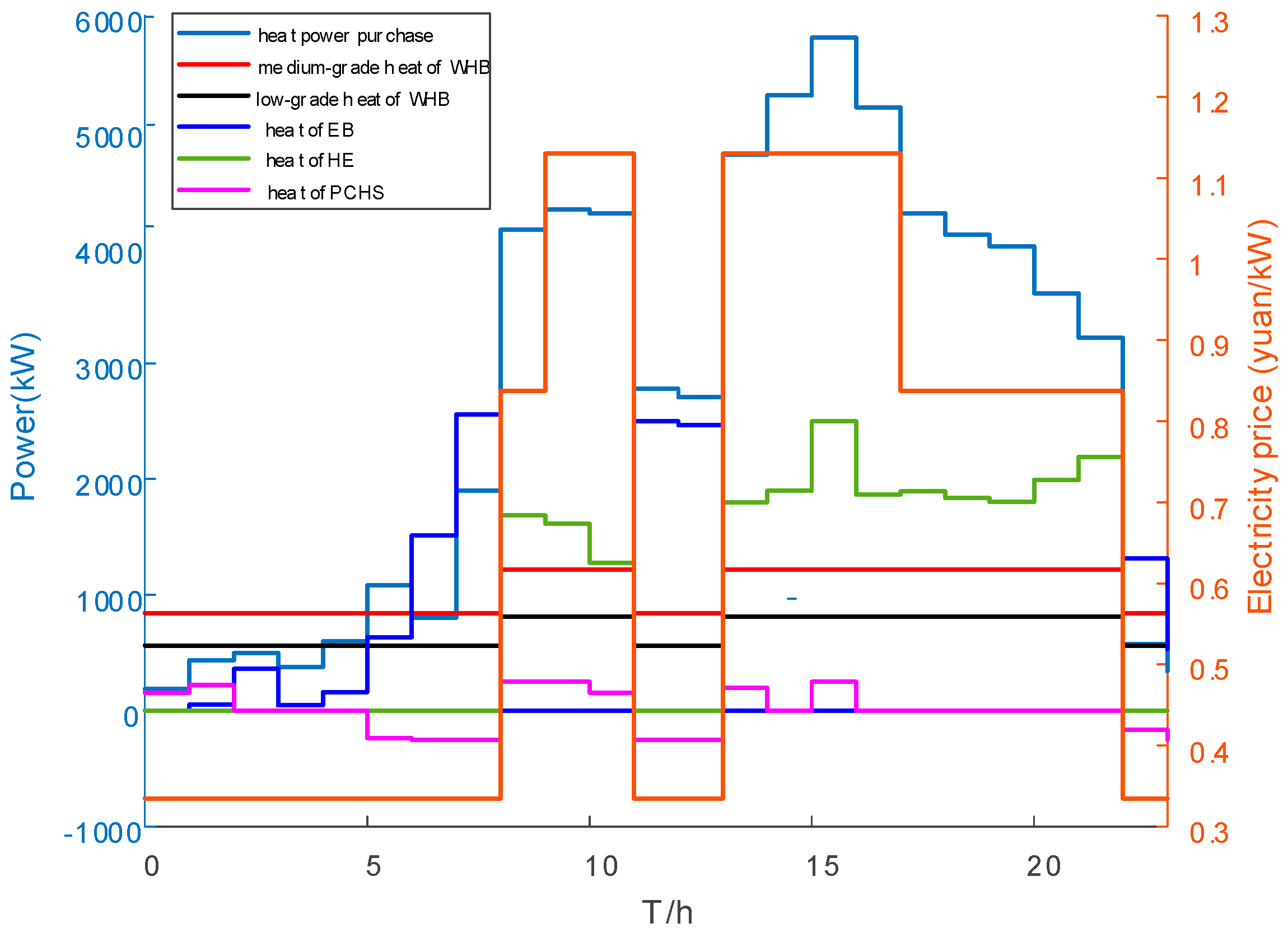
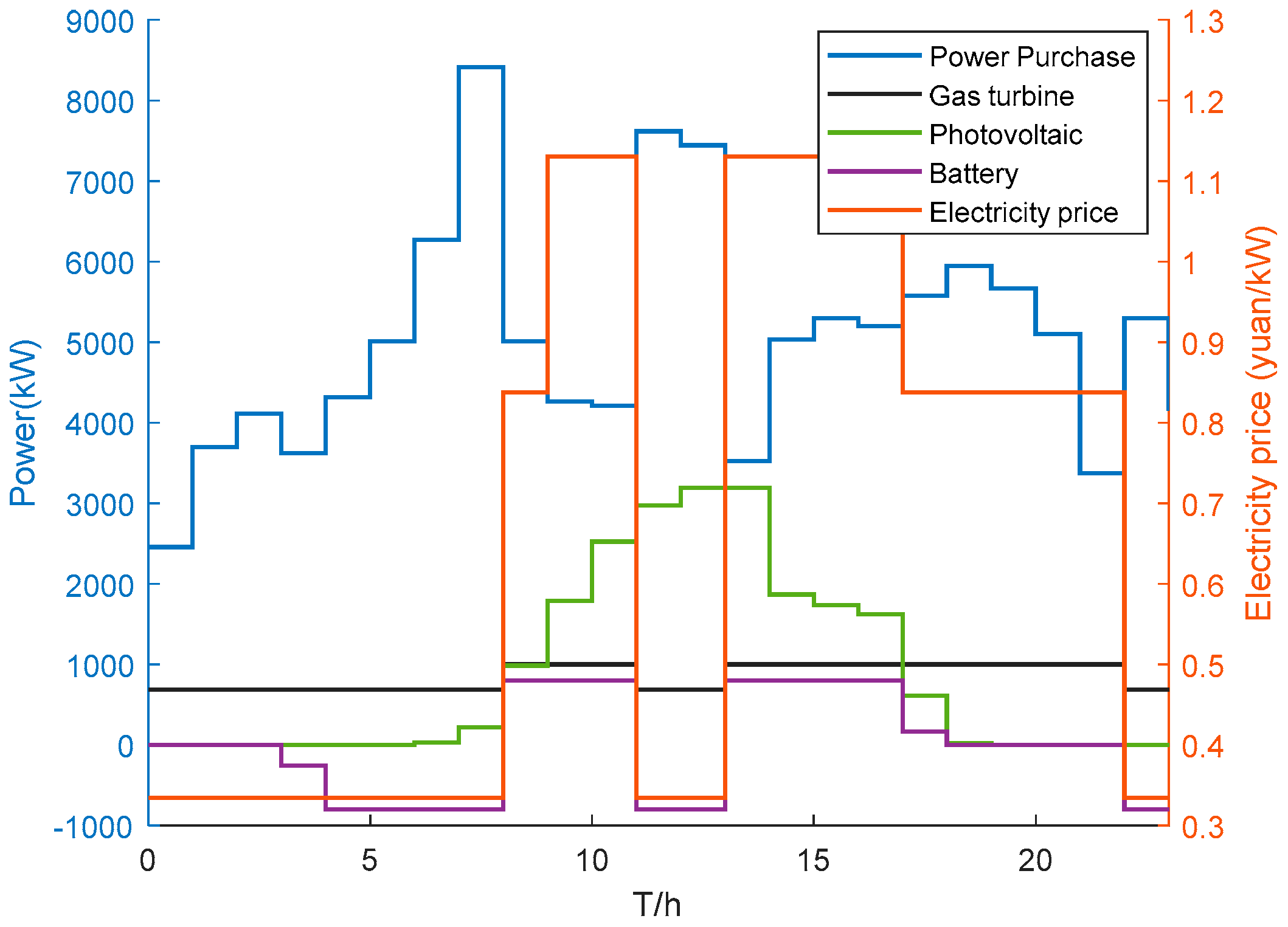
4.2. Price-Based Comprehensive Demand Response Results

The CPLEX12.8 optimization software was used to solve the results of the time-of-use electricity price optimization operation of the micro-energy grid’s participation in the price-based comprehensive demand response. Figure 3 shows the optimal operation results of the power supply system of the micro-energy grid, where time 1 corresponds to 0:00. It can be seen from the figure that photovoltaic power generation is 100% consumed, and the gas turbine is in the trough electricity price period from 22:00 to 8:00 the next day. From 11:00 to 13:00, the power generation is 691.75 kW, and the full power generation is 1000 kW during peak and peak hours. This is because the power generation cost of gas turbines is higher than the time-of-use electricity price during valley hours. Additionally, battery energy storage is charged at 3:00–8:00 and 11:00–13:00 during the trough hours, and at 22:00, during peak electricity prices, and discharged at peak 8:00–11:00, with 13:00–17:00, through the electricity price peak-to-valley arbitrage to further reduce the operating cost of the micro-energy grid in the peak. At the peak hours of electricity prices, the overall power purchase of the micro-energy grid decreases.

Figure 4 displays the optimal operational results of the micro-energy grid heating system. The medium-grade and low-grade thermal power output by the waste heat boiler primarily depend on the electrical power output by the gas turbine. The heat accumulator stores heat during the trough period of electricity price, releasing it from 8:00 to 11:00 during peak hours and from 13:00 to 14:00. The electric boiler operates during peak hours of electricity price from 8:00 to 11:00 and from 13:00 to 21:00. Heat exchangers do not produce low-grade heat. Instead, they only produce heat during peak and off-peak hours of electricity prices. This is because electric heating is more expensive during peak hours than the cost of using medium-grade heat exchange. Conversely, during off-peak hours, electric heating is cheaper than the cost of using medium-grade heat exchange. By using this complementary approach, the operating cost of the micro-energy grid can be further reduced.

When comparing the results of the micro-energy grid with and without ice storage air conditioner participation, the daily operating cost was CNY 133,439.05 and CNY 133,452.61, respectively, after the price-based integrated demand response. Ice storage air conditioners generally have a lifespan of over 15 years. It has been determined that their lifespan is specifically 15 years, resulting in a time-sharing tariff arbitrage of CNY 74,241. Additionally, participating in peak demand response can reduce the peak by 130 kW, 30 times a year, resulting in a peak subsidy of CNY 234,000. The total estimated gain is CNY 308,241. Equipping the micro-energy grid with an ice storage air-conditioner costing CNY 200,000 can recover the investment cost and generate revenue.

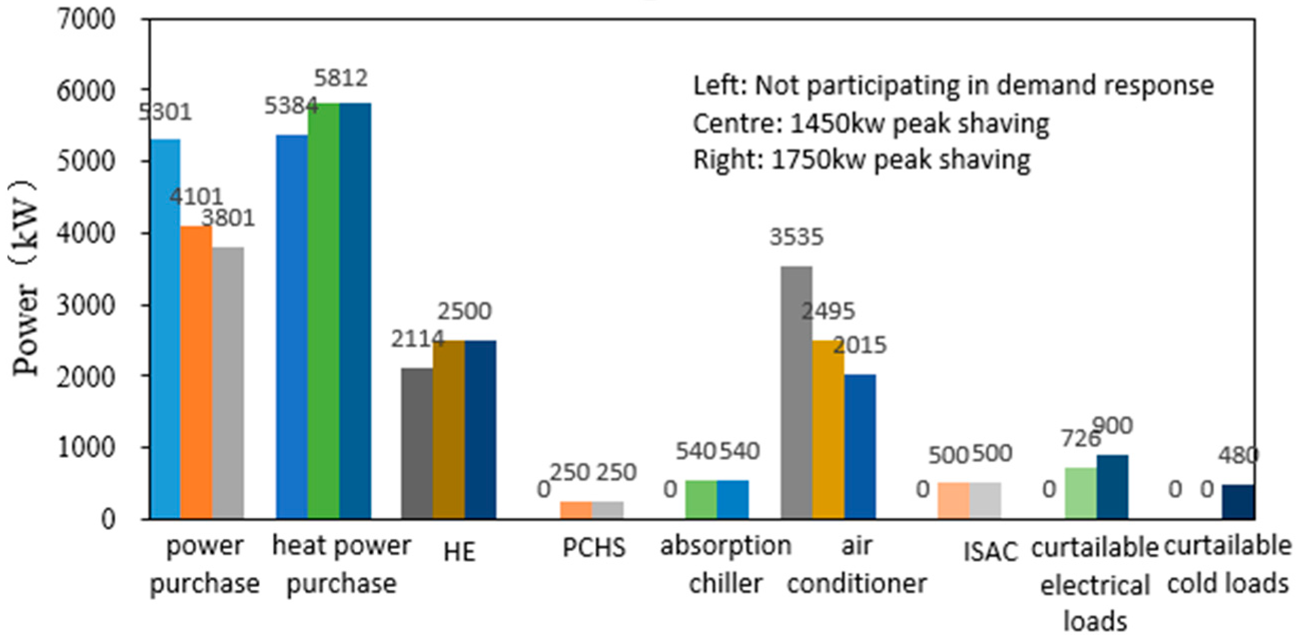
4.3. Incentivized Comprehensive Demand Response Results

Considering the two types of peak shaving demand issued by the power grid: peak shaving of 1200 kW during the 15:00–16:00 period and peak shaving of 1500 kW during the 15:00–16:00 period, the comparison of the operation of the micro-energy grid before and after participating in the incentive demand response is shown in Figure 5 below.

Figure 5 shows three bars for each item, representing the relevant equipment within the micro-energy network before participating in incentivized demand response, peak shaving of 1450 kW, and peak shaving of 1750 kW. It is evident that the electric refrigeration air conditioner generates significantly less cooling power after participating in the incentive-based integrated demand response. Additionally, peak shaving of 1750 kW results in a greater reduction in output power compared to peak shaving of 1450 kW, which effectively reduces power consumption. The decrease in cooling power of the electric refrigeration air conditioner is compensated for by the ice storage air conditioner and the absorption chiller. These systems melt and cool the ice at their maximum output power. The absorption chiller starts from its original shutdown cooling at full output power using low-grade heat. As a result, the purchased heat demand of the micro-energy network increases, the heat converted by the heat exchanger increases, and the heat accumulators release heat at maximum power. In regard to dispatchable loads, the cost of peak shaving for the electrically transferable load is CNY 1.38, with the lowest response cost. During the 15:00–16:00 period, 450 kW of electric load is transferred to the 0:00–1:00 tariff trough period, and the thermally levelling load does not contribute to peak shaving and does not respond to it. The electrically curtailable load is reduced by 726 kW during peak shaving of 1450 kW and by 900 kW during peak shaving of 1750 kW. The cold curtailable load has a higher response cost than the electric curtailable load and exceeds the peaking subsidy, so it is not curtailed at a peak shaving of 1450 kW. However, it is curtailed by 480 kW at a peak shaving of 1750 kW.

Based on the analysis above, it can be concluded that the micro-energy network described in this paper effectively utilizes its demand response potential through various energy storage methods, dispatchable loads, and multi-energy complementarity of electricity, heat, and cold. Additionally, it can reduce energy costs by participating in incentive-based demand response programs.

5. Conclusions

In this paper, we propose a comprehensive demand response optimization strategy for micro-energy grids considering the dispatchable load. Considering the cascade utilization of thermal energy, a typical micro-energy grid structure including electricity, gas, medium-grade heat, low-grade heat, and cold energy is constructed. A comprehensive energy equipment model is established, including a variety of energy storage models: battery energy storage, phase change heat storage, ice-cold storage device, and a refined scheduling model that can reduce load and transfer load, and a convert load is given. On this basis, taking the operation economy of the micro-energy grid as the optimization goal, considering the constraints of new energy consumption rate and energy supply reliability, a comprehensive demand response strategy of the micro-energy grid participating in the electricity price type and incentive type is proposed.

Through the analysis of the examples, the following conclusions can be obtained:

(1)

The price-based comprehensive demand response strategy of micro-energy grid proposed in this paper can optimize the energy consumption structure of a micro-energy grid under the guidance of time-of-use electricity price, reduce operating costs, and ensure the consumption of new energy. For the power grid, the peak-to-valley difference can be reduced to achieve a win–win situation.

(2)

The incentive-based comprehensive demand response strategy of the micro-energy grid proposed in this paper enables the micro-energy grid to minimize its own costs while responding to the peak regulation demand of the upper level and obtain the peak shaving subsidy to further reduce its own operating cost. The proposed strategy fully excavates the demand response potential of the micro-energy grid through dispatchable load; the complementarity of electricity, heat, and cold realizes the comprehensive coordination and optimization of source–grid–load–storage, provides greater peak regulation capacity, and obtains greater benefits when participating in the incentive-based comprehensive demand response. Thus, it provides theoretical reference and support for the majority of multi-energy users to participate in the comprehensive demand response.

(3)

The method proposed in this paper can estimate whether the investment cost can be recovered by the micro-energy grid during the life cycle of the phase change heat accumulator and ice-cold storage device; additionally, it can provide a reference for the energy storage planning of the micro-energy grid. For the case of the micro-energy grid in this example, compared with the case of only electrochemical energy storage, the economic benefit and lower net cost of the micro-energy grid participating in the comprehensive demand response with the configuration of ice storage device are greater.

This paper deeply explores the integrated demand response potential of micro-energy networks and proposes a method with good engineering practicality. However, the paper acknowledges that the method still has deficiencies. The paper presents an MINLP problem model that is challenging to solve. It can be applied to solve small-scale micro-energy network systems. However, as the system scale expands and equipment increases, the algorithm’s complexity, computational resources, and required time also increase significantly. Therefore, when calculating demand response solutions for larger energy networks, we propose that one tries to consider the micro-energy network as a whole and establish a centralized–distributed mechanism. This will allow for joint optimization of the regional integrated energy system through participation with multiple micro-energy networks in incentive-based demand response.

References

1. Xue, Y.; Yu, X. Beyond smart grid cyber physical social system in energy future. Proc. IEEE 2017, 105, 2290. [Google Scholar] [CrossRef]
2. Yong, L.; Yao, Z.; Yi, T.; Cao, Y.; Bu, F. Optimal stochastic operation of integrated low carbon electric power, natural gas and heat delivery system. IEEE Trans. Sustain. Energy 2018, 9, 273–283. [Google Scholar]
3. Chen, X.; Wang, C.; Wu, Q.; Dong, X.; Yang, M.; He, S.; Liang, J. Optimal operation of integrated energy system considering dynamic heat-gas characteristics and uncertain wind power. Energy 2020, 198, 117270. [Google Scholar] [CrossRef]
4. Jia, H.J.; Wang, D.X. Research on Some Key Problems Related to Integrated Energy Systems. Autom. Electr. Power Syst. 2015, 39, 198–207. [Google Scholar]
5. Wang, J. Planning and Optimal Operation of Regional Integrated Energy System. Master’s Thesis, Southeast University, Nanjing, China, 2017. [Google Scholar]
6. Lv, J.W.; Zhang, S.X.; Cheng, H.Z. A review of regional integrated energy system planning research considering interconnection and interaction. Proc. CSEE 2021, 41, 4001–4021. [Google Scholar]
7. Xu, Z.; Sun, H.B.; Guo, Q.L. Review and Prospect of Integrated Demand Response. Proc. CSEE 2018, 38, 7194–7205+7446. [Google Scholar]
8. Palensky, P.; Dietrich, D. Demand side management: Demand response, intelligent energy systems, and smart loads. IEEE Trans. Ind. Inform. 2011, 7, 381–388. [Google Scholar] [CrossRef]
9. Tian, S.; Wang, B.; Zhang, J. Key technologies for demand response under smart grid conditions. Proc. CSEE 2014, 34, 3576–3589. [Google Scholar]
10. Sheikhi, A.; Bahrami, S.; Ranjbar, A.M. An autonomous demand response program for electricity and natural gas networks in smart energy hubs. Energy 2015, 89, 490–499. [Google Scholar] [CrossRef]
11. Sun, Y.J.; Wang, Y.; Wang, B.B. Multi-time scale decision method for source-load interaction considering demand response uncertainty. Autom. Electr. Power Syst. 2018, 42, 106–113, 159. (In Chinese) [Google Scholar]
12. Ding, Y.R.; Chen, H.K.; Wu, J. Multi-objective optimal dispatch of electricity-gas-heat integrated energy system considering comprehensive energy efficiency. Autom. Electr. Power Syst. 2021, 45, 64–73. (In Chinese) [Google Scholar]
13. Wei, J.D.; Zhang, Y.; Wang, J.X. Decentralized demand management based on alternating direction method of multipliers algorithm for industrial park with CHP units and thermal storage. J. Mod. Power Syst. Clean Energy 2022, 10, 120–130. [Google Scholar] [CrossRef]
14. Xu, H.; Dong, S.F.; He, Z.X. Electro-thermal comprehensive demand response based on multi-energy complementarity. Power Syst. Technol. 2019, 43, 480–487. [Google Scholar] [CrossRef]
15. Zhang, D.; Zhu, H.; Zhang, H. Multi-objective optimization for smart integrated energy system considering demand responses and dynamic prices. IEEE Trans. Smart Grid 2022, 13, 1100–1112. [Google Scholar] [CrossRef]
16. Tian, S.M.; Luan, W.P.; Zhang, D.X. Energy Internet Technology Form and Key Technologies. Proc. CSEE 2015, 35, 3482–3494. [Google Scholar]
17. Yang, H.H.; Shi, B.W.; Huang, W.T. Optimal Scheduling Method for Micro Energy Grids Based on Integrated Demand Response. Electr. Power Constr. 2021, 42, 11–19. [Google Scholar]
18. Zhu, L.; Niu, P.Y.; Tang, L.J. Robust optimization operation of micro-energy network considering the uncertainty of direct load control. Power Syst. Technol. 2020, 44, 1400–1413. [Google Scholar]
19. Huang, C.; Zhang, H.; Song, Y.; Wang, L.; Ahmad, T.; Luo, X. Demand response for industrial micro-grid considering photovoltaic power uncertainty and battery operational cost. IEEE Trans. Smart Grid 2021, 12, 3043–3055. [Google Scholar] [CrossRef]
20. Chen, Z.; Zhang, Y.; Tang, W. Generic modelling and optimal day-ahead dispatch of micro-energy system considering the price-based integrated demand response. Energy 2019, 176, 171–183. [Google Scholar] [CrossRef]
21. Chen, J.; Qi, B.; Rong, Z.; Peng, K.; Zhao, Y.; Zhang, X. Multi-energy coordinated microgrid scheduling with integrated demand response for flexibility improvement. Energy 2021, 217, 119387. [Google Scholar] [CrossRef]
22. Sheikhahmadi, P.; Bahramara, S.; Mazza, A.; Chicco, G.; Shafie-Khah, M.; Catalão, J.P.S. Multi-Microgrids Operation with Interruptible Loads in Local Energy and Reserve Markets. IEEE Syst. J. 2023, 17, 1292–1303. [Google Scholar] [CrossRef]
23. Bahramara, S.; Mazza, A.; Chicco, G.; Shafie-Khah, M.; Catalão, J.P. Comprehensive review on the decision-making frameworks referring to the distribution network operation problem in the presence of distributed energy resources and microgrids. Int. J. Elect. Power Energy Syst. 2020, 115, 105466. [Google Scholar] [CrossRef]
24. Sun, C.H.; Wang, L.J.; Xu, H.L. User interaction load modelling and its application to microgrid day-ahead economic dispatch. Power Syst. Technol. 2016, 40, 2009–2016. [Google Scholar]
25. Hosseini, S.M.; Carli, R.; Parisio, A.; Dotoli, M. Robust Decentralized Charge Control of Electric Vehicles under Uncertainty on Inelastic Demand and Energy Pricing. In Proceedings of the 2020 IEEE International Conference on Systems, Man, and Cybernetics (SMC), Toronto, ON, Canada, 11–14 October 2020; pp. 1834–1839. [Google Scholar] [CrossRef]
26. Xu, Y.; Peng, S.; Liao, Q.; Yang, Z.; Liu, D.C.; Zou, H. Two-stage short-term optimal dispatch of MEP considering CAUR and HTTD. Electr. Power Autom. Equip. 2017, 37, 152–163. [Google Scholar]
27. Ma, T.F.; Wu, J.; Hao, L.L. Energy Flow Modeling and Optimal Operation Analysis of Micro Energy Grid Based on Energy Hub. Power Syst. Technol. 2018, 42, 179–186. [Google Scholar] [CrossRef]
Figure 1. Micro-energy grid energy supply structure.
Energies 17 01255 g001
Figure 2. Micro-energy grid PV output and load forecast results before the day.
Energies 17 01255 g002
Figure 3. The optimization operation results of power supply system.
Energies 17 01255 g003
Figure 4. The optimization operation results of heating system.
Energies 17 01255 g004
Figure 5. Comparison chart of the operation of the micro-energy grid before and after participating in the incentivized comprehensive demand response.
Energies 17 01255 g005