Abstract
Efficient management of renewable energy resources is imperative for promoting environmental sustainability and optimizing the utilization of clean energy sources. This paper presents a pioneering European-scale study on energy management within renewable energy communities (RECs). With a primary focus on enhancing the social welfare of the community, we introduce a reinforcement learning (RL) controller designed to strategically manage Battery Energy Storage Systems (BESSs) and orchestrate energy flows. This research transcends geographical boundaries by conducting an extended analysis of various energy communities and diverse energy markets across Europe, encompassing different regions of Italy. Our methodology involves the implementation of an RL controller, leveraging optimal control theory for training and utilizing only real-time data available at the current time step during the test phase. Through simulations conducted in diverse contexts, we demonstrate the superior performance of our RL agent compared to a state-of-the-art rule-based controller. The agent exhibits remarkable adaptability to various scenarios, consistently surpassing existing rule-based controllers. Notably, we illustrate that our approach aligns with the intricate patterns observed in both Italian and European energy markets, achieving performance levels comparable to an optimal controller assuming perfect theoretical knowledge of future data.
1. Introduction
In recent times, renewable energy sources have gained attention as a sustainable alternative to traditional fossil fuels. Fueled by goals outlined for ecological transition, such as those outlined in the European Agenda 2030 [1], there is a growing focus on renewable resources. The rise of communities dedicated to sustainable energy, often portrayed as agents of change with significant benefits for participants [2], has prompted the need for a carefully structured framework to facilitate the integration of these sources into the power grid. As delineated in [3], renewable energy communities (RECs) are coalitions of individuals and entities collaborating to advocate and employ renewable energy sources, encompassing solar, wind, and hydroelectric power. This collective effort promotes the adoption and utilization of environmentally friendly energy alternatives. These entities exist in various forms, from small clusters of residents collectively funding solar panel installations to large-scale organizations driving communal renewable energy initiatives. The primary goal of RECs is to enhance the overall social welfare of the community (refer to the formal explanation below). This encompasses managing the expenses and income associated with energy transactions within the community and with the broader grid. A crucial component of the necessary infrastructure is the Battery Energy Storage System (BESS), which plays a vital role in balancing energy supply and demand.
Addressing this challenge has seen the application of diverse techniques such as traditional optimization methods, heuristic algorithms, and rule-based controllers [4,5]. Notably, the mixed-integer linear programming (MILP) solution has demonstrated considerable success in energy management applications. In [6], the authors addressed the problem of managing an energy community hosting a fleet of electric vehicles for rent. The request-to-vehicle assignment requires the solution of a mixed-integer linear program. In [7], the authors presented an optimized MILP approach specifically aimed at improving the social welfare of a REC, a parameter that embraces revenues from the energy sold to the grid, costs for energy bought from the grid, costs for battery usage, and potential incentives for self-consumption. However, effectively scheduling BESS charging/discharging policies encounters a critical hurdle due to the pronounced intermittency and stochastic nature of renewable generation and electricity demand [8]. Accurately predicting these uncertain variables proves to be a formidable task, and this is where machine learning-based strategies come into play [9,10]. Alternatively, to address this issue, uncertainty-aware optimization techniques have been developed, such as stochastic programming (SP) and robust optimization (RO) [11]. SP employs a probabilistic framework but requires a priori knowledge of the probability distribution to model the uncertainties, whereas RO focuses on the worst-case scenario and, therefore, requires the known bounds of the uncertainties, leading to far more conservative performance. On the flip side, an alternative strategy for real-time scheduling, such as model predictive control (MPC), introduced in [12], has emerged. MPC continuously recalibrates its solution in a rolling-horizon fashion. Although beneficial, the effectiveness of the MPC solution is contingent upon the precision of forecasts [13]. Moreover, the substantial online computational load of long-horizon MPC in extensive systems poses a potential hurdle for real-time execution. Hence, there is a notable shift in focus toward methodologies rooted in deep reinforcement learning (DRL). In recent years, DRL has gained substantial relevance in diverse energy management applications [14,15,16]. Addressing the distinctive constraints inherent in power scheduling poses a significant challenge for DRL approaches. An uncomplicated strategy involves integrating constraints into the reward function as soft constraints [17]. To tackle this issue, approaches based on imitation learning (IM) have been suggested. In [18], the agent learns directly from the trajectories of an expert (specifically, an MILP solver). Despite the commendable outcomes, these approaches often overlook the incentive for virtual self-consumption proposed in the Italian framework. In [19], an interactive framework for benchmarking DRL algorithms was presented; however, it is not reflective of REC behavior and incentive schemes. Furthermore, the primary objective typically revolves around flattening consumption curves (benefiting energy suppliers), as observed in [14], rather than maximizing the social welfare of the community.
In our previous work [20], we introduced a novel DRL strategy for managing energy in renewable energy communities. This strategy introduces an intelligent agent designed to maximize social welfare through real-time decision making, relying only on currently available data, thus eliminating the necessity for generation and demand forecasts. To enhance the agent’s training effectiveness, we leverage the MILP approach outlined in [7] by directly incorporating optimal control policies within an asymmetric actor–critic framework. Through diverse simulations across various REC setups, we demonstrate that our methodology surpasses a state-of-the-art rule-based controller. Additionally, it yields BESS control policies with performance closely matching the optimally computed ones using MILP. In this study, we have expanded our research scope to encompass a broader framework that addresses the entire European landscape. By doing so, we aim to shed light on the advantages of our study in a more comprehensive context. This extended perspective allows us to offer insights into the applicability and benefits of our innovative DRL approach not only within individual RECs but also on a larger scale, contributing to a more sustainable and efficient energy landscape across Europe.
1.1. Hypothesis of This Study
This study focuses on efficiently managing renewable energy resources to promote sustainability and optimize clean energy usage. Our primary hypothesis centers on the potential for RL controllers to significantly enhance energy management within RECs. Specifically, we posit that the strategic utilization of RL, particularly in the orchestration of BESSs, can lead to substantial improvements in social welfare within these communities. By transcending geographical boundaries and conducting a comprehensive examination of various energy communities and markets across Europe, we aim to test the hypothesis that RL controllers, grounded in optimal control theory and utilizing real-time data, can outperform existing rule-based controllers. Through extensive simulations in diverse contexts, we seek to demonstrate the adaptability of our proposed RL agent to various scenarios and its ability to achieve performance levels comparable to an optimal controller with perfect theoretical knowledge of future data. This hypothesis forms the basis of our investigation into advancing sustainable energy management strategies across European regions.
1.2. Enhancing Novelty: Methodological Advancements and Unexplored Territories
This study unfolds with a distinctive focus on augmenting the novelty of our research methodologies and delving into previously unexplored territories within the realm of renewable energy management. This study employs sophisticated simulation frameworks, specifically designed within the OpenAI Gym, to replicate real-world REC dynamics. Additionally, this study broadens its geographical scope to encompass diverse energy communities and markets across Italy and Europe, providing insights into regional variations and unexplored complexities. The methodological innovations and exploration of uncharted territories in this study establish a strong foundation for future research efforts. By pushing the boundaries of current understanding in the field, this study sets a precedent for integrating cutting-edge methodologies into renewable energy studies.
1.3. Regional Variations in Energy Dynamics: Insights from Italian Regions and beyond
Understanding REC dynamics requires analyzing regional variations in energy dynamics. The inclusion of various regions within Italy serves as a crucial aspect of our study, providing insights into the specific challenges and opportunities within the Italian energy landscape. Italy’s diverse geographical and socio-economic characteristics necessitate a tailored approach to energy management, making it an ideal testing ground for our proposed reinforcement learning (RL) controller. On the other hand, extending our analysis to countries beyond Italy, such as France, Switzerland, Slovenia, and Greece, adds a transnational dimension to our research. The selection of these specific countries is grounded in their diverse energy market structures, regulatory frameworks, and renewable energy adoption rates. France, with its nuclear-heavy energy mix, offers a contrasting scenario to Italy’s reliance on renewables. Switzerland, a country known for its hydropower capacity, provides insights into decentralized energy systems. Slovenia and Greece, with their unique geographical characteristics, contribute to a more comprehensive understanding of REC dynamics in southern Europe. By incorporating this diverse set of countries, we aim to capture a broad spectrum of challenges and opportunities faced by different European regions. This comparative analysis enhances the generalizability of our findings, allowing us to extrapolate insights that are not only relevant to Italy but also applicable to a broader European context. The careful selection of these countries aligns with our goal of providing a holistic perspective on the application of RL controllers in optimizing energy management across diverse geographical and regulatory landscapes.
This work proceeds as follows. Section 2 encompasses a review of the relevant literature. Section 3 formalizes the task and introduces our methodology. Section 4 delineates the simulations and illustrates the numerical outcomes. Finally, Section 5 concludes the discussion, delving into potential future advancements.
2. Related Works
Given our interest in the European perspective and the aim to compare various countries, we examine energy communities operating under an incentive framework akin to the one embraced in Italy. Within this context, the Italian government ensures incentives for virtual self-consumption within a renewable energy community, as described in [21,22,23]. Virtual self-consumption is defined as “the minimum, in each hourly period, between the electricity produced and fed into the network by renewable energy plants and electricity taken from all final customers associates”.
Most research efforts focus on managing shared energy among community members and optimizing economic outcomes. This includes analyzing storage system scheduling and maximizing incentives. For example, the framework presented in [24] delved into a scenario featuring a photovoltaic (PV) generation facility, a BESS, and a central user entity representing all community consumers connected to the public grid. This configuration allows for a streamlined analysis, focusing on the aggregate community virtual self-consumption rather than individual instances, with the incentives attained subsequently calculated retrospectively. Another contribution can be found in [25], where the authors proposed a model considering various generators and consumers, with a central BESS acting as a community member. In the community framework examined in [8], there are exclusive consumers alongside a single prosumer equipped with a PV installation and a BESS. Strict limitations are enforced to ensure the BESS charges solely from the PV system and to prevent simultaneous charging and discharging (utilizing binary variables), thereby avoiding arbitrage situations resulting from self-consumption incentives.
Paper’s Contributions
This paper explores the application of reinforcement learning to renewable energy communities within an incentive framework. In this context, community members maintain their contracts with energy providers and buyers and receive incentives for the virtual self-consumption achieved at the community level. A centralized scheme is considered, where entities share consumption and generation information to maximize overall community welfare, including the incentive. This analysis extends beyond Italy, encompassing various European states to provide a comparative perspective and account for diverse situations. The significance of this study lies in its broad examination of RECs across European states, offering insights into reinforcement learning’s applicability in diverse regulatory environments. The collaborative, centralized approach enhances energy management efficiency, optimizes community welfare, and promotes sustainability. The focus on community-level incentives adds realism, addressing the interconnected nature of REC operations.
This paper builds upon a conference paper [20]. Here, we provide more details regarding the adopted methodology and extend the validation to new datasets from several European countries.
3. Methods
In this section, we outline the problem formulation, control techniques employed, designed architecture, optimization procedure, and simulated environment used.
3.1. Problem Formulation
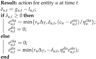
Suppose an energy community consists of U entities, each including a load, a generator, and a Battery Energy Storage System (BESS). A centralized energy controller is responsible for computing the scheduling of the BESS. At each time step t, the controller chooses an action for the BESS of each entity u. These actions, denoted by values in the range of [−1, 1], represent the fraction of the rated power for charging or discharging the BESS.
The amounts of energy charged to and discharged from the battery of entity u at time t are computed as follows:
To account for physical constraints, actions at each time step are bounded as follows:
Consequently, the action space of the controller is continuous and within the range of [, ], where positive values indicate BESS charging and negative values indicate discharging.
The energy controller’s objective is to select actions that maximize the daily social welfare of the community. This welfare is defined by the following equation:
This equation encompasses the revenues from energy sold to the grid, costs for energy bought from the grid, costs for battery usage, and incentives for virtual self-consumption. Notice that the min term in (5) represents the virtual community self-consumption, as defined in [21].
The objective is to maximize (5) with respect to feasible actions while adhering to constraints like BESS dynamics, energy balance, and complementarity constraints, ensuring non-simultaneous export to and import from the grid for each entity. For more details, interested readers can refer to [7,26]. To ensure that the community’s operation is decoupled on different days, an additional constraint is imposed: the BESSs must be fully discharged at the beginning and end of each day.
3.2. Optimal Control Policy
As discussed in [7], the optimization problem in Section 3.1 is non-convex due to complementarity constraints of the type:
These constraints enforce that there is no simultaneous import and export with the grid for each entity of the community at each time period. To address this issue, an equivalent MILP formulation was proposed in [7]. The formulation requires binary variables for each entity and for each time step to determine the direction of the energy exchange with the grid. It is stressed that when the demand and generation profiles are the true ones, the MILP provides the optimal BESS control policy. While assuming to have an oracle is not realistic in practice, in this paper, we make a twofold use of the optimal BESS control policy computed with the MILP: first, to aid in agent training within an actor–critic structure, and second, to assess the performance of the proposed DRL approach on fresh data not used for training.
3.3. Reinforcement Learning Approach
The MILP formulation presented in Section 3.2 necessitates the solution of daily demand and generation profiles (or their forecasts). In this section, we introduce a deep reinforcement learning (DRL) approach that determines the next actions based solely on the currently available information.
To achieve this, the problem described in Section 3.1 is cast as a classical reinforcement learning (RL) problem. RL is an agent-based algorithm that learns through interaction with the environment it controls [27,28] (see Figure 1).
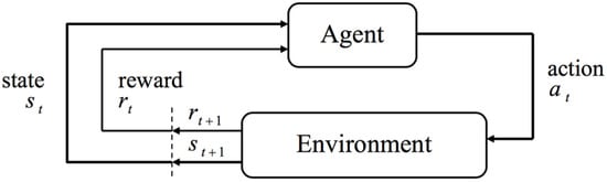
Figure 1.
Agent–environment interaction in RL framework.
The objective of the agent (referred to as the energy controller) is to maximize the expected cumulative sum of discounted rewards over time. RL is formalized using a Markov Decision Process (MDP), represented by a tuple , where P is a state transition probability matrix, denoting the probability that action a in state s at time t leads to state at time :
R is a reward function expressing the expected reward received after transitioning from state s to state with action a:
and [0, 1] is a discount factor for future rewards. The policy represents a mapping between states and actions, , describing the behavior of an agent.
RL is further formalized using a Markov Decision Process (MDP), which includes the sets of states S and actions A, a reward function , and transition probabilities between states ∈ [0, 1]. The policy represents a mapping between states and actions, , and the value function is the expected return for the agent starting in state s and following policy , i.e.,
where , denoted as r(s,a), is the reward obtained after taking action , transitioning from the current state s to the next state s′, and [0, 1] is a discount factor for future rewards.
We designate the energy controller as the typical reinforcement learning (RL) agent, which, by iteratively engaging with an environment E across independent episodes and discrete-time steps, receives input observations and rewards and generates actions . As previously stated, the agent’s objective is to maximize the daily welfare of the community by taking actions every hour. The agent operates without relying on forecasting data, as it only has access to current time-step information. In our context, captures only a portion of the true hidden state of the problem, i.e., the data for the entire day. Consequently, the environment E is characterized as a Partially Observable Markov Decision Process (POMDP). The classical RL paradigm is impractical for this scenario because modeling the action space would necessitate computing all possible state–action combinations.
To address these challenges, we leverage Deep Neural Network (DNN) approximators and adopt the actor–critic formulation. Specifically, our goal is to learn an actor model that provides the optimal policy for the given task and a critic model responsible for evaluating such a policy. Both the actor and the critic are implemented using two distinct DNNs: a Policy-DNN (the actor network) and a Value-DNN (the critic network). The latter is active only during the training phase, whereas the Policy-DNN is the actual model used during testing to determine actions. Instead of employing traditional symmetric actor–critic implementations, where the two DNNs share the same inputs, we adopt an asymmetric structure. Inputs to the Policy-DNN are segregated into global data, common to all entities, and individual data from each entity. Prior to being fed into the network, the inputs undergo preprocessing. Table 1 summarizes the data constituting the state of the Policy-DNN.

Table 1.
Policy-DNN state.
Since the critic operates exclusively during the training phase, the structure of the asymmetric actor–critic offers an opportunity to impart additional supervised information, which is more challenging to acquire during testing, to the critic network. Specifically, in addition to the inputs presented to the actor, we furnish the Value-DNN with the optimal action computed for the load and generation data corresponding to that precise time step. Assuming no stochasticity in the training data for the agent (as actions impact only a portion of the state, i.e., the state of charge of the batteries), this information is readily derived for the training data through the optimal control optimization procedure detailed in Section 3.2. By incorporating this information about the optimal action achievable at that time step into the network, we empower the critic to more effectively evaluate the actions undertaken by the actor.
3.4. Actor–Critic Architecture
The Policy-DNN, as illustrated in Figure 2, processes the preprocessed data (referred to as the actor’s state) outlined in Table 1. This neural network employs five fully connected layers, and each layer undergoes layer normalization over a mini-batch of inputs, following the approach detailed in [29]. The U outputs produced by the final layer correspond to the actions for the U entities. All layers, excluding the output layer, incorporate ReLu activation. The number of neurons in each layer is depicted in Figure 2.
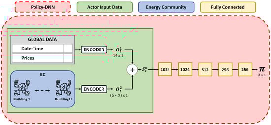
Figure 2.
Illustration of the architecture of the Policy-DNN utilized in this study, showcasing the input sizes derived from both global and individual data after preprocessing. The Policy-DNN consists of approximately 1.8 million parameters, which may vary based on the community’s size. The preprocessing step, critical for model preparation, is visually represented in the figure, with the green block indicating the current state and refined input sizes fed into the fully connected layers for decision making.
In contrast, in addition to receiving the same actor data, the Value-DNN (see Figure 3) is supplemented with the U optimal actions for the current time step. These optimal actions are computed for the entire day’s generation and consumption data using the optimal control algorithm outlined in Section 3.2. Similar to the Policy-DNN, the Value-DNN comprises five fully connected layers, incorporating ReLu activation and layer normalization. The final layer of the Value-DNN outputs the scalar value .
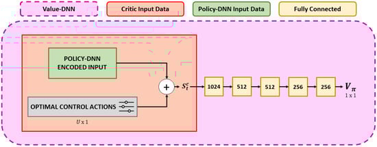
Figure 3.
The visual representation within the red block provides an insightful overview of the architecture of the Value-DNN. This model receives the same inputs as the Policy-DNN and additionally receives optimal actions computed beforehand using the MILP algorithm for the current time step. The optimal actions do not require additional encoding, as they are naturally bounded within the interval [−1, 1]. The state depicted in the red box undergoes processing by a sequence of fully connected layers to calculate the value function.
3.5. Optimization Procedure
In our scenario, the objective is to train a centralized deep reinforcement learning (DRL) agent with the capability to manage the scheduling of Battery Energy Storage Systems (BESSs) in an effort to maximize the daily social welfare (5) within the energy community. To accomplish this goal, our algorithm incorporates the following two primary features:
- Exploitation of optimal control actions: During the training phase, we have access to optimal actions computed using the MILP algorithm outlined in Section 3.2. We leverage this information to enhance our agent’s training. By feeding the optimal actions as input to the Value-DNN, we aim to improve the critic’s ability to evaluate the actions taken by the actor.
- Reward penalties for constraint violations: At each time step, the Policy-DNN of the agent generates U actions, each corresponding to a specific entity. As the training objective is to maximize social welfare, we utilize the social welfare for that time step as the reward signal for the actor’s actions. The Policy-DNN’s output actions are in the range of [−1, 1]. Each action is then scaled by the rated power (i.e., ) of the BESS of the corresponding entity to determine the actual power for charging/discharging the storage systems. Each action is then multiplied by the rated power (i.e., ) of the BESS of the corresponding entity to obtain the actual power for charging/discharging the storage systems. However, the actor’s actions may violate feasibility constraints. In such cases, actions that do not comply with the constraints are replaced with physically feasible actions, and a penalty is computed for the constraint violation for each action () using (10):The resulting total penalty is the average of the individual penalties:This overall penalty is subtracted from the reward, resulting in the following reward signal, which is used to train the agent:where is the social welfare (5) computed for the current time step and is a training hyperparameter. By providing - and as inputs to the networks and using such a reward signal, our agent is capable of both maximizing social welfare and learning actions that do not violate physical constraints. It is indeed not uncommon to use DRL algorithms to train a single model to solve different tasks in parallel.
The models undergo optimization using the well-known Soft Actor–Critic (SAC) algorithm [30]. As a method operating off-policy, SAC effectively utilizes a replay buffer [31] to recycle experiences and derive insights from a reduced sample pool. SAC is built upon three fundamental features: an actor–critic architecture, off-policy updates, and entropy maximization. The algorithm learns three distinct functions: the actor (policy), the critic (soft Q-function), and the value function V defined as:
where is the Shannon entropy of the policy . In the context of state , this entropy is the probability distribution of all possible actions available to the agent. A policy with zero entropy is deterministic, implying that all actions, except the optimal one , have zero probability = 1. Policies with non-zero entropy enable more randomized action selection, enhancing exploration and avoiding premature convergence to suboptimal policies. The SAC agent’s objective is to learn the optimal stochastic policy , given by:
The deterministic nature of the final optimal policy is achieved by simply choosing the expected action of the policy (mean of the distribution) as the action of choice, as performed in the evaluation of our agents after training. Here, represents a state–action pair sampled from the agent’s policy and is the reward for that particular state–action pair. Due to the inclusion of the entropy term, the agent endeavors to maximize returns while exhibiting behavior that is as random as possible. The critic network’s parameters undergo updates by minimizing the expected error between the predicted Q-values and those calculated through iteration, expressed as:
In Equations (13) and (14), the hyperparameter is denoted as the temperature. This parameter plays a pivotal role in influencing the significance of the entropy term and, consequently, the stochasticity of the learned policy. Specifically, setting would emphasize behaving as stochastically as possible, potentially resulting in uniformly random behavior. Conversely, when , the entropy is disregarded, directing the agent to prioritize maximizing the return without exploration, thereby leading to an almost deterministic policy. For a more comprehensive understanding of the Soft Actor–Critic (SAC) algorithm, we direct interested readers to the relevant literature [30]. It is noteworthy that the parameters for the policy and the value function differ due to the utilization of an asymmetric actor–critic paradigm.
3.6. Simulation Environment
Throughout our investigation, the development of a simulated environment emerged as a critical component tailored specifically to facilitate the training of our intelligent agent. This simulation tool, meticulously crafted in accordance with the recognized standards of OpenAI Gym [32], stands as a sophisticated platform designed to emulate the intricate dynamics inherent to a renewable energy community operating within an incentive framework. Within this simulated REC environment, we considered a variable number of entities denoted by U, with each entity potentially equipped with solar panels for energy generation and an associated electrical storage system. The flexibility of our simulation setup is a noteworthy feature, allowing for the granular customization of the REC’s configuration. Parameters such as the number of entities, power output of the solar panels, and capacity of the Battery Energy Storage Systems (BESSs) are all user-defined, facilitating a diverse range of scenarios for the agent to navigate and learn from. As depicted in Figure 4, the simulated environment operates on a discrete-time basis, reflecting the temporal dynamics of real-world REC dynamics. At each discrete-time step, the environment receives a set of actions computed by our DRL agent. These actions, which dictate the charging or discharging power for each individual BESS within the community, are integral to steering the energy flows and optimizing overall system performance. The simulation process then unfolds as the environment responds to these actions by updating its state information, encapsulating the current energy status of each entity and the community as a whole. Additionally, a reward signal is generated at each time step, as defined by Equation (12). This reward signal encapsulates the feedback mechanism for the DRL agent, serving as a quantitative measure of the efficacy of its actions in alignment with the overarching goal of optimizing social welfare within the REC. This dynamic feedback loop encapsulates the iterative learning process of the DRL agent, allowing it to continually adapt and optimize its decision-making strategies over successive time steps. The incorporation of this carefully crafted simulated environment ensures a controlled yet realistic setting for training the agent, enabling a robust evaluation of its performance under diverse and dynamically evolving scenarios. The versatility and fidelity of our simulation design contribute to the reliability and generalizability of the insights gained from the subsequent analysis of the agent’s performance.
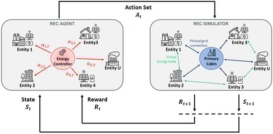
Figure 4.
In the framework, the agent–environment interaction occurs in multiple steps. Initially, the agent calculates actions based on the current state, denoted as , for each building. These actions reflect the agent’s decisions. Subsequently, the Gym environment checks whether the actions comply with the constraints. Any violations result in penalties, which are factored into the overall reward signal. The environment then computes the community’s social welfare, a key component of the reward signal, reflecting the societal impact of the agent’s decisions. Thus, the reward signal includes penalties for constraint violations and the calculated social welfare, serving as a quantitative feedback mechanism. Finally, the environment provides the agent with the calculated reward and the new state calculated from the current state and the agent’s actions.
3.7. Reinforcement Learning Logic Concept
In this section, we present an overview of the reinforcement learning logic concept. For this purpose, we present a graphical representation (see Figure 5) illustrating the approach used to train our RL agent and highlighting the various components detailed in the previous sections.
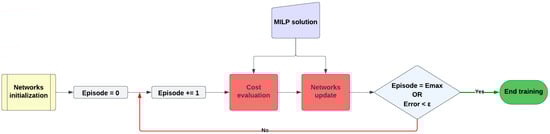
Figure 5.
Flowchart illustrating the training logic of the reinforcement learning agent.
The training phase commences with the initialization of the neural networks within the RL agent, specifically the Policy-DNN and Value-DNN detailed in Section 3.4. Subsequently, the training loop is initiated, operating episodically, with each iteration incrementing the episode counter. Within each episode, two primary operations occur: cost evaluation, assessing the agent’s capacity to maximize social welfare, and neural network updates. Interacting with the virtual environment outlined in Section 3.6, the agent receives a reward signal based on its policy-driven actions. As shown in Equation (12), the reward is inclusive of social welfare, which is used precisely as a cost function to evaluate the agent’s performance. Throughout training, the optimal MILP solution, computed a priori with perfect knowledge of future data, serves a dual purpose. Firstly, it assesses cost by comparing the RL agent’s performance against the MILP approach’s optimal performance, setting an upper bound. Secondly, the neural network update phase is performed using the SAC algorithm, as described in Section 3.5. In this phase, MILP solutions are used in the Value-DNN to train the critic. A double condition is checked at the end of each iteration. Training is terminated either when the episode count reaches the maximum limit or when the discrepancy between the costs obtained with the RL agent and those from MILP falls below a predefined threshold (a training parameter).
4. Results
Our simulations were designed to evaluate the agent’s ability to optimize social welfare, as expressed by Equation (5), within the energy community. To demonstrate the generalization capabilities and effectiveness of our proposed approach, experiments were conducted across various scenarios and conditions.
4.1. Dataset Selection and Rationale
In our investigation, we carefully curated data from 11 diverse regions across Italy and Europe to simulate various configurations of renewable energy communities. These regions encompassed a mix of geographical locations, each with unique characteristics influencing energy dynamics. Included were northern and southern Italy, specific Italian islands, and European nations such as Slovenia, Switzerland, Greece, and France. To ensure a robust representation of energy consumption scenarios, we leveraged datasets provided CityLearn [19] to simulate building consumption. These datasets enabled the simulation of different building types, ranging from industrial facilities to retail establishments and households. This diverse set of building profiles ensured a comprehensive exploration of REC dynamics, considering the varied energy needs and consumption patterns across different sectors. For generation data, we relied on PVGIS, a reliable source offering accurate information on photovoltaic generation potential. This choice was motivated by the need for precise and region-specific generation data to capture the nuances of each zone’s renewable energy potential. In terms of energy prices, we aimed for realism by considering actual market conditions. Zone-specific energy sale prices for 2022 were sourced from the GME (Gestore Mercati Elettrici) website, providing real-world market rates. The choice of specific pricing structures, such as hourly bands for Italian zones and fixed rates for France, Switzerland, Slovenia, and Greece, reflects the diverse energy market dynamics in these regions. This meticulous approach to data selection ensured that our simulation captured the intricacies of each region, facilitating a nuanced analysis of REC performance and behavior under varying conditions.
In the pursuit of comprehending the dynamics of RECs across diverse regions in Italy and Europe, we present visual representations that offer invaluable insights into two pivotal aspects: annual photovoltaic production and energy purchase/sale prices.
Production across Six Zones
The first visual aid encapsulates the annual production in six distinct zones. This graphical representation presents the AC inverted power (W) on the ordinate axis and spans across the months on the abscissa. Through this visual narrative, we aim to provide a comprehensive depiction of daily fluctuations in energy generation. By juxtaposing these figures, readers can discern the geographical nuances influencing the production landscape and appreciate the temporal dynamics inherent in renewable energy sources.
Energy Purchase and Sale Prices in Four Zones
The second visual representation delves into the intricate dynamics of energy markets by showcasing the purchase and sale prices across four zones. This comparative view offers a nuanced understanding of the economic factors shaping REC operations by providing a condensed narrative of the energy market’s history, including daily fluctuations and peak periods. With buying and selling prices as the focal points, this visual aid provides a snapshot of the economic landscape within which these communities operate, facilitating an insightful analysis of market trends and regional disparities.
These visuals, coupled with our meticulous dataset selection process, lay the foundation for the exploration of RECs’ behavior and performance. They not only enhance the reader’s understanding of regional disparities but also set the stage for a comprehensive analysis of the interconnected factors shaping the renewable energy landscape across diverse European contexts.
4.2. Training Details
The Policy-DNN and Value-DNN were trained with an SAC agent over 150 episodes, employing the Adam optimizer [33] with learning rates of and , respectively, and a batch size of 512. Each episode consisted of one year of hourly sampled data, totaling 8760 steps, and ended at the end of the year. The penalty coefficient of the reward (i.e., ) was set to 10 and the discount factor to 0.99. We clipped the gradient norm at 40 for all the networks. The SAC parameter and the temperature coefficient were set to and 0.1, respectively. We used a replay buffer with a maximum capacity of trajectories.
4.3. Evaluation Scenarios, Baselines, and Metrics
We assessed the performance of our methodology across diverse setups of the energy community. In each configuration, we modified the community’s parameters, including the number of entities, generation and consumption profiles, prices for the purchase and sale of energy, and sizing of the photovoltaic arrays and storage systems. In particular, we analyzed RECs designed in 11 different areas distributed among Italian regions and European countries (see Figure 6):
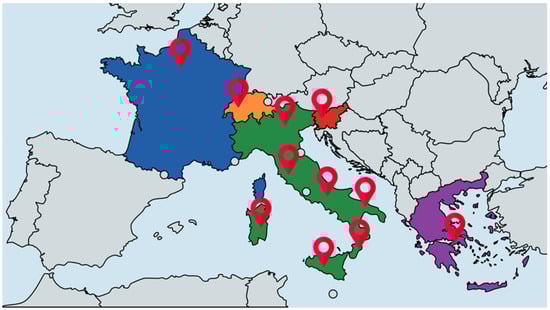
Figure 6.
Positions of energy communities among European states: 7 RECs in different Italian regions, and 1 REC for each capital in France, Switzerland, Slovenia, and Greece.
- 1.
- FRAN: France, Paris;
- 2.
- SVIZ: Switzerland, Berne;
- 3.
- SLOV: Slovenia, Ljubljana;
- 4.
- GREC: Greece, Athens;
- 5.
- NORD: northern Italy;
- 6.
- CNORD: central-northern Italy;
- 7.
- CSUD: central-southern Italy;
- 8.
- SUD: southern Italy;
- 9.
- CALA: Calabria region, Italy;
- 10.
- SICI: Sicily island, Italy;
- 11.
- SARD: Sardinia island, Italy.
In each zone, the generation and consumption profiles, as well as the purchase and sale prices, varied, as described in Section 4.1. The performance of our approach was evaluated in four configurations of the energy community, including 3, 5, 7, and 9 entities. As shown in Table 2, for each configuration, we used the data of one climate zone for training, and then we tested the agent on two different climate zones.
Table 2.
Climate zones used for each energy community.
Table 3 shows the sizes of the photovoltaic systems (kWp) and storage systems (kWh) for the buildings in the different types of communities.
Table 3.
Production and storage system sizing for each energy community.
Throughout both the training and testing phases, we benchmarked our agent against two baseline energy controllers:
- Optimal Controller (OC), as detailed in Section 3.2. The optimal scheduling of the BESSs for each day was determined using a mixed-integer linear programming (MILP) algorithm. This approach assumes complete knowledge of generation and consumption data for all 24 h, yielding optimal actions for BESS control and maximizing the daily community welfare.
- Rule-Based Controller (RBC). The BESSs’ actions were determined by predefined rules following Algorithm 1. Rule-based controllers, as exemplified in Algorithm 1, are commonly employed to schedule the charge and discharge policies of storage systems. For each entity, the RBC controller charged the BESS with surplus energy as long as the battery had not reached maximum capacity. Conversely, if less energy was produced than required, the loads were supplied with the energy from the BESS, if available.
| Algorithm 1: Rule-based controller action selection |
 |
Given that the primary objective of the energy controller is to maximize daily social welfare, we evaluated our agent’s performance by comparing the social welfare achieved by the RL controller’s actions with that achieved by the baseline controllers. The OC solution served as an upper limit (optimal solution), representing the best possible results. Therefore, we assessed our agent’s performance by determining how closely it approached the optimal solution. Similarly, we also evaluated the performance difference when using the RBC controller instead of the OC controller.
The trend of daily social welfare over a one-year period is depicted by a non-stationary time series. We contend that calculating the ratio between the OC, RL, and RBC time series may lead to misleading results. This is due to the fact that comparing small values of welfare may yield small differences but high ratios. For this reason, to quantitatively measure the performance of the compared approaches, we introduced the following metric:
Fit Score: This metric measures the similarity between two time series and by returning the fit score between them, defined as:
In our context, always represents the OC series, providing the best possible solution achieved with an oracle providing perfect forecasts. Meanwhile, represents either the RL or the RBC series. This approach allowed us to assess how close our method was to the optimal solution and, simultaneously, how much better our method performed compared to a rule-based controller.
4.4. Results Discussion
The outcomes of the simulations are documented in Table 4. For each trial conducted across diverse community configurations, the table displays the fit scores between the OC controller and the alternative energy controllers. Notably, our approach (RL) consistently outperformed the rule-based controller and achieved results comparable to the performance of the optimal controller, representing the upper limit. These outcomes stem directly from the learned policy of social welfare maximization by our agent.
Table 4.
Train and test results for each energy community configuration.
It is important to note that the data on generation, consumption, and energy purchase and sale prices (see Figure 7 and Figure 8) varied significantly across the various areas where energy communities were simulated (refer to Table 2). These results indeed underscore the agent’s capacity to generalize the learned policy even in previously unseen contexts, distinct from the scenarios encountered in the training phase.
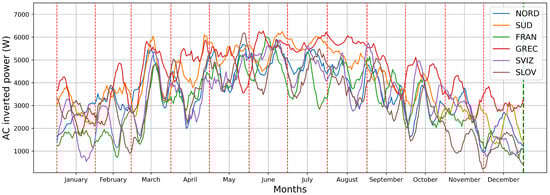
Figure 7.
Monthly distribution of PV generation in six distinct zones. The detailed visualization highlights the high variability among the different geographic areas considered in this study.
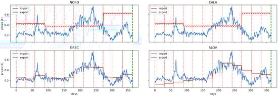
Figure 8.
Daily dynamics of energy market transactions. The figure displays the purchase (import) and sale (export) prices in four distinct zones. The x-axis plots the progression of days, providing a chronological perspective, whereas the y-axis quantifies prices in EUR, providing a standardized metric for evaluation.
Upon scrutinizing the performance of the RBC in various energy community configurations, it became evident that in some scenarios, the RBC controller achieved very poor results. This phenomenon can be attributed to the fact that the use of a controller based on trivial rules is not suitable for an extremely dynamic environment where prices change hourly based on the energy market. It is noteworthy that, unlike RBC, the RL agent managed to maintain almost consistent performance, even with an increasing number of entities and the use of data from different areas, thereby significantly outperforming the rule-based controller.
5. Conclusions
Our study introduces a novel experimental strategy for BESS scheduling in energy communities. We propose a reinforcement learning agent capable of maximizing the social welfare of the community using only current time-step data, without relying on data forecasts. Through extensive experiments, we show that our approach surpasses the performance of a state-of-the-art (SotA) rule-based controller and achieves results comparable to an optimal MILP controller that assumes perfect knowledge of future data. Experiments demonstrate how our agent reaches good performance in vastly different application scenarios, where energy consumption, production data, and purchase and sale prices can vary greatly. Importantly, our study spans geographical boundaries, encompassing a comprehensive examination of various energy communities and diverse energy markets across Europe, including different regions of Italy. The observed performance of our RL agent aligns seamlessly with the intricate patterns characterizing both Italian and European energy markets. This not only validates the viability of RL-based approaches in practical energy management scenarios but also emphasizes the potential impact of our findings on advancing sustainable energy utilization strategies across diverse European regions.
Implications and Limitations of this Study
Our study on energy management within renewable energy communities offers valuable insights with both theoretical and practical implications. The utilization of reinforcement learning controllers demonstrates promising outcomes for optimizing social welfare within RECs. The theoretical implications highlight the efficacy of RL-based approaches in navigating the complex and dynamic nature of energy systems, emphasizing their adaptability and performance advantages over traditional rule-based systems. Practically, our study provides actionable insights for policymakers, energy planners, and community stakeholders. The performance of the RL agent across diverse scenarios in European regions suggests its potential as a practical tool for enhancing energy management efficiency. Its adaptability to different market patterns in both Italian and European contexts reinforces its versatility in real-world applications. Our research extends implications to other studies in the field of renewable energy and smart grid management. The findings suggest RL controllers as a viable solution for optimizing energy flows. However, acknowledging the limitations of our study is essential. Although the regional scope provides valuable insights, it may not capture the full spectrum of global energy dynamics. Further research could explore the application of RL controllers in different cultural and regulatory contexts. Additionally, addressing the assumption of perfect theoretical knowledge of future data in the optimal controller scenario by incorporating more realistic forecasting methods may be vital for future studies.
In conclusion, our study quantifies significant contributions to the field of renewable energy management. Our approach achieves performance levels comparable to an optimal controller with perfect theoretical knowledge, emphasizing its tangible impact on advancing sustainable energy utilization strategies. The adaptability of our agent to different market patterns is reflected in its robust performance, providing a quantified measure of its effectiveness.
In future work, we aim to conduct experiments in energy community scenarios with even more entities involved, transitioning from a centralized solution to a more scalable distributed solution based on the promising federated reinforcement learning technique.
Author Contributions
Conceptualization, G.P. and L.G.; Software, L.G. and M.S.; Validation, G.P. and A.R.; Writing—original draft, G.P. and L.G.; Writing—review & editing, A.R. and S.P.; Supervision, S.P. All authors have read and agreed to the published version of the manuscript.
Funding
This research was funded by grant under the FRESIA project.
Data Availability Statement
Data available on request due to restrictions eg privacy or ethical.
Conflicts of Interest
Authors Giulia Palma and Leonardo Guiducci declare that a portion of their research was financially supported by Sunlink Srl. The funder was not involved in the study design, collection, analysis, interpretation of data, the writing of this article or the decision to submit it for publication. The authors declare no conflicts of interest.
Abbreviations
The following abbreviations are used in this manuscript:
| REC | Renewable Energy Community |
| BESS | Battery Energy Storage System |
| PV | Photovoltaic |
| RL | Reinforcement Learning |
| DRL | Deep Reinforcement Learning |
| DNN | Deep Neural Network |
| SAC | Soft Actor–Critic |
| RBC | Rule-Based Controller |
| OC | Optimal Control |
| MILP | Mixed-Integer Linear Programming |
| Constants and sets | |
| U | number of entities forming the community |
| T | number of time periods per day |
| duration of a time period (h) | |
| S | set of states |
| A | set of actions |
| Variables | |
| energy imported from the grid by entity u at time t (kWh) | |
| energy exported to the grid by entity u at time t (kWh) | |
| energy level of the battery of entity u at time t (kWh) | |
| energy supplied to the battery of entity u at time t (kWh) | |
| energy withdrawn from the battery of entity u at time t (kWh) | |
| Parameters | |
| maximum capacity of the battery of entity u (kWh) | |
| energy generated by PV plant of entity u at time t (kWh) | |
| energy demand of entity u at time t (kWh) | |
| rated power of the battery of entity u (kW) | |
| discharging efficiency of battery of entity u | |
| charging efficiency of battery of entity u | |
| unit price of energy exported to the grid by entity u at time t (EUR/kWh) | |
| unit price of energy imported from the grid by entity u at time t (EUR/kWh) | |
| unitary cost for usage of energy storage of entity u at time t (EUR/kWh) | |
| unit incentive for community self-consumption at time t (EUR/kWh) | |
References
- United Nations. Agenda 2030. Available online: https://tinyurl.com/2j8a6atr (accessed on 28 January 2024).
- Gjorgievski, V.Z.; Cundeva, S.; Georghiou, G.E. Social arrangements, technical designs and impacts of energy communities: A review. Renew. Energy 2021, 169, 1138–1156. [Google Scholar] [CrossRef]
- Directive (EU) 2018/2001 of the European Parliament and of the Council on the promotion of the use of energy from renewable sources. Off. J. Eur. Union 2018, 328, 84–209. Available online: https://eur-lex.europa.eu/legal-content/EN/TXT/PDF/?uri=CELEX:32018L2001 (accessed on 28 January 2024).
- Parhizi, S.; Lotfi, H.; Khodaei, A.; Bahramirad, S. State of the Art in Research on Microgrids: A Review. IEEE Access 2015, 3, 890–925. [Google Scholar] [CrossRef]
- Zia, M.F.; Elbouchikhi, E.; Benbouzid, M. Microgrids energy management systems: A critical review on methods, solutions, and prospects. Appl. Energy 2018, 222, 1033–1055. [Google Scholar] [CrossRef]
- Zanvettor, G.G.; Casini, M.; Giannitrapani, A.; Paoletti, S.; Vicino, A. Optimal Management of Energy Communities Hosting a Fleet of Electric Vehicles. Energies 2022, 15, 8697. [Google Scholar] [CrossRef]
- Stentati, M.; Paoletti, S.; Vicino, A. Optimization of energy communities in the Italian incentive system. In Proceedings of the 2022 IEEE PES Innovative Smart Grid Technologies Conference Europe (ISGT-Europe), Novi Sad, Serbia, 10–12 October 2022; pp. 1–5. [Google Scholar]
- Talluri, G.; Lozito, G.M.; Grasso, F.; Iturrino Garcia, C.; Luchetta, A. Optimal battery energy storage system scheduling within renewable energy communities. Energies 2021, 14, 8480. [Google Scholar] [CrossRef]
- Aupke, P.; Kassler, A.; Theocharis, A.; Nilsson, M.; Uelschen, M. Quantifying uncertainty for predicting renewable energy time series data using machine learning. Eng. Proc. 2021, 5, 50. [Google Scholar]
- Liu, L.; Zhao, Y.; Chang, D.; Xie, J.; Ma, Z.; Sun, Q.; Yin, H.; Wennersten, R. Prediction of short-term PV power output and uncertainty analysis. Appl. Energy 2018, 228, 700–711. [Google Scholar] [CrossRef]
- Chen, Z.; Wu, L.; Fu, Y. Real-Time Price-Based Demand Response Management for Residential Appliances via Stochastic Optimization and Robust Optimization. IEEE Trans. Smart Grid 2012, 3, 1822–1831. [Google Scholar] [CrossRef]
- Parisio, A.; Rikos, E.; Glielmo, L. A Model Predictive Control Approach to Microgrid Operation Optimization. IEEE Trans. Control. Syst. Technol. 2014, 22, 1813–1827. [Google Scholar] [CrossRef]
- Palma-Behnke, R.; Benavides, C.; Lanas, F.; Severino, B.; Reyes, L.; Llanos, J.; Sáez, D. A Microgrid Energy Management System Based on the Rolling Horizon Strategy. IEEE Trans. Smart Grid 2013, 4, 996–1006. [Google Scholar] [CrossRef]
- Vazquez-Canteli, J.R.; Henze, G.; Nagy, Z. MARLISA: Multi-Agent Reinforcement Learning with Iterative Sequential Action Selection for Load Shaping of Grid-Interactive Connected Buildings. In Proceedings of the 7th ACM International Conference on Systems for Energy-Efficient Buildings, Cities, and Transportation, Yokohama, Japan, 18–20 November 2020. [Google Scholar] [CrossRef]
- Bio Gassi, K.; Baysal, M. Improving real-time energy decision-making model with an actor-critic agent in modern microgrids with energy storage devices. Energy 2023, 263, 126105. [Google Scholar] [CrossRef]
- Ji, Y.; Wang, J.; Xu, J.; Fang, X.; Zhang, H. Real-Time Energy Management of a Microgrid Using Deep Reinforcement Learning. Energies 2019, 12, 2291. [Google Scholar] [CrossRef]
- Mocanu, E.; Mocanu, D.C.; Nguyen, P.H.; Liotta, A.; Webber, M.E.; Gibescu, M.; Slootweg, J.G. On-Line Building Energy Optimization Using Deep Reinforcement Learning. IEEE Trans. Smart Grid 2019, 10, 3698–3708. [Google Scholar] [CrossRef]
- Gao, S.; Xiang, C.; Yu, M.; Tan, K.T.; Lee, T.H. Online Optimal Power Scheduling of a Microgrid via Imitation Learning. IEEE Trans. Smart Grid 2022, 13, 861–876. [Google Scholar] [CrossRef]
- Vázquez-Canteli, J.R.; Dey, S.; Henze, G.; Nagy, Z. CityLearn: Standardizing Research in Multi-Agent Reinforcement Learning for Demand Response and Urban Energy Management. arXiv 2020, arXiv:2012.10504. [Google Scholar]
- Guiducci, L.; Palma, G.; Stentati, M.; Rizzo, A.; Paoletti, S. A Reinforcement Learning approach to the management of Renewable Energy Communities. In Proceedings of the 2023 12th Mediterranean Conference on Embedded Computing (MECO), Budva, Montenegro, 6–10 June 2023; pp. 1–8. [Google Scholar] [CrossRef]
- Legge 28 Febbraio 2020, n. 8, Recante Disposizioni Urgenti in Materia di Proroga di Termini Legislativi, di Organizzazione Delle Pubbliche Amministrazioni, Nonché di Innovazione Tecnologica. Gazzetta Ufficiale n. 51. 2020. Available online: https://www.gazzettaufficiale.it/eli/id/2020/02/29/20G00021/sg (accessed on 28 January 2024).
- Autorità di Regolazione per Energia Eeti e Ambiente. Delibera ARERA, 318/2020/R/EEL—Regolazione delle Partite Economiche Relative all’Energia Condivisa da un Gruppo di Autoconsumatori di Energia Rinnovabile che Agiscono Collettivamente in Edifici e Condomini oppure Condivisa in una Comunità di Energia Rinnovabile. 4 August 2020. Available online: https://www.arera.it (accessed on 28 January 2024).
- Decreto Ministeriale 16 Settembre 2020—Individuazione Della Tariffa Incentivante per la Remunerazione Degli Impianti a Fonti Rinnovabili Inseriti Nelle Configurazioni Sperimentali di Autoconsumo Collettivo e Comunità Energetiche Rinnovabili. Gazzetta Ufficiale n. 285. 2020. Available online: https://www.mimit.gov.it/it/normativa/decreti-ministeriali/decreto-ministeriale-16-settembre-2020-individuazione-della-tariffa-incentivante-per-la-remunerazione-degli-impianti-a-fonti-rinnovabili-inseriti-nelle-configurazioni-sperimentali-di-autoconsumo-collettivo-e-comunita-energetiche-rinnovabili (accessed on 28 January 2024).
- Cielo, A.; Margiaria, P.; Lazzeroni, P.; Mariuzzo, I.; Repetto, M. Renewable Energy Communities business models under the 2020 Italian regulation. J. Clean. Prod. 2021, 316, 128217. [Google Scholar] [CrossRef]
- Moncecchi, M.; Meneghello, S.; Merlo, M. A game theoretic approach for energy sharing in the italian renewable energy communities. Appl. Sci. 2020, 10, 8166. [Google Scholar] [CrossRef]
- Stentati, M.; Paoletti, S.; Vicino, A. Optimization and Redistribution Strategies for Italian Renewable Energy Communities. In Proceedings of the IEEE EUROCON 2023—20th International Conference on Smart Technologies, Torino, Italy, 6–8 July 2023; pp. 263–268. [Google Scholar] [CrossRef]
- Sutton, R.S.; Barto, A.G. Reinforcement Learning: An Introduction, 2nd ed.; The MIT Press: Cambridge, MA, USA, 2018. [Google Scholar]
- Rizzo, A.; Burgess, N. An action based neural network for adaptive control: The tank case study. In Towards a Practice of Autonomous Systems; MIT Press: Cambridge, MA, USA, 1992; pp. 282–291. [Google Scholar]
- Ba, J.L.; Kiros, J.R.; Hinton, G.E. Layer normalization. arXiv 2016, arXiv:1607.06450. [Google Scholar]
- Haarnoja, T.; Zhou, A.; Abbeel, P.; Levine, S. Soft Actor-Critic: Off-Policy Maximum Entropy Deep Reinforcement Learning with a Stochastic Actor. arXiv 2018, arXiv:1801.01290. [Google Scholar]
- Wang, Z.; Bapst, V.; Heess, N.; Mnih, V.; Munos, R.; Kavukcuoglu, K.; de Freitas, N. Sample Efficient Actor-Critic with Experience Replay. arXiv 2017, arXiv:1611.01224. [Google Scholar]
- Brockman, G.; Cheung, V.; Pettersson, L.; Schneider, J.; Schulman, J.; Tang, J.; Zaremba, W. OpenAI Gym. arXiv 2016, arXiv:1606.01540. [Google Scholar]
- Kingma, D.P.; Ba, J. Adam: A Method for Stochastic Optimization. arXiv 2017, arXiv:1412.6980. [Google Scholar]
Disclaimer/Publisher’s Note: The statements, opinions and data contained in all publications are solely those of the individual author(s) and contributor(s) and not of MDPI and/or the editor(s). MDPI and/or the editor(s) disclaim responsibility for any injury to people or property resulting from any ideas, methods, instructions or products referred to in the content. |
© 2024 by the authors. Licensee MDPI, Basel, Switzerland. This article is an open access article distributed under the terms and conditions of the Creative Commons Attribution (CC BY) license (https://creativecommons.org/licenses/by/4.0/).