Wind Turbine Blade Damage Evaluation under Multiple Operating Conditions and Based on 10-Min SCADA Data

Abstract

The present paper aims to enable the assessment of the fatigue damage of wind turbine blades over a long duration (e.g., several months/years) in conjunction with different operating regimes and based on two information sources: the 10-min SCADA data and an interpolation using response surfaces identified using the FAST aeroelastic numerical tool. To assess blade damage, prior studies highlighted the need for a high-frequency (>1 Hz) sampling rate. Because of data availability and computation resource limitations, such methods limit the duration of the analysis period, making the direct use of such an approach based on a 1 Hz wind speed signal in current wind farms impractical. The present work investigates the possibility of overcoming these issues by estimating the equivalent damage using a 1 Hz wind speed for each 10-min sample stored in the SCADA data. In the literature, the influence of operating regimes is not considered in fatigue damage estimation, and for the first time, the present project takes a pioneering approach by considering these operating regimes.

1. Introduction

To support ever-growing energy needs worldwide, the market share taken up by wind energy electricity production is expected to grow from the current 5% to 45% by 2050 [1]. One of the key drivers enabling this increase is the levelized cost of energy (LCOE). The cost of wind turbine (WT) energy production is expected to drop by 30% between 2020 and 2050, and the optimization of operation and maintenance (O&M) strategies will be crucial when it comes to ensuring this LCOE drop. O&M costs linked to wind turbine blades (WTBs) are very significant because the WTB failure rate due to fatigue is particularly high [2,3] and the replacement cost for the blades is quite prohibitive [4,5]. That is why this study focuses on the assessment of WTB fatigue damage.

Several methods exist for assessing WTB damage [6]. For instance, thermal imaging involves identifying temperature variations along the blade to detect delamination or cracks [7]. Another method is ultrasonic scanning, where an ultrasonic wave is sent into the blade and deviations or reflections indicate defects. The defect can then be located and measured by analyzing the response time and amplitude of the outgoing ultrasonic wave [8]. Additionally, damage detection can be achieved by monitoring the noise produced when damage occurs in the WTB (cracks, delamination, etc.) using sensors. Each type of defect corresponds to a distinct noise pattern, allowing for the determination of the defect’s position, severity, and type [9]. Many other methods for detecting damage exist [6]. However, all these methods often require installation of specific equipment on wind turbines or immobilization of turbines for blade diagnostics [6].

That’s why current research efforts focus largely on the predictive maintenance relying on existing equipment. The predictive maintenance of WTBs could optimize their associated O&M costs and ultimately assess the possibility of WT life extension. Predictive maintenance is intended to prevent elevated corrective action and repair costs associated with reactive maintenance. There are presently two main categories of predictive maintenance available [10], the first of which relies on a data-driven approach and includes a predictive maintenance model based on an exponential expression of WTB damage behavior [11]. The other was inspired by a Bayesian dynamic network and discretizes WTB damage into several levels. Within this model, the transition from one damage step to the next is driven by a probability law. The main advantage of data-driven models is that they can provide a damage assessment in a computationally efficient manner [10,11]. Nevertheless, such models are limited by the need for hard-to-find parameters which are essential for a reliable assessment of the remaining useful life (RUL).

The second predictive maintenance category relies on physical models such as the FASTIGUE process developed by Eder & Chen (2020) [12]. A number of such physical models already allow for the computation of the WTB RUL. Models based on the Miner’s rule are most commonly used because of their simplicity of operation [13,14,15,16,17,18,19,20,21,22,23,24]. There are other approaches available, but these are less commonly used due to their inherent limitations. As an example, damage models that rely on the Walker or Paris–Erdogan elastic crack propagation law require the application of a pre-existing crack [10,12,25]. One advantage presented by physical models is that they provide accurate estimations of damage behavior. Nevertheless, the use of physical damage models is extremely time-consuming when applied to the entire lifetime of a WT (generally 20 to 30 years). Moreover, physical damage models require a 1 Hz wind speed (WS) sampling frequency to achieve a reliable WTB damage computation, given the high sensitivity of WTBs to WS fluctuations at this frequency, as explained by Jang et al. [17]. Consequently, because 1 Hz WS SCADA data is very heavy and fatigue assessment via physical damage models can be time-consuming, a WTB damage assessment cannot be carried out for extended time periods [17]. Another problem is that 1 Hz frequency SCADA data is rarely used by wind farm operators, given that the IEC 61400-12-1 standard [26] recommends using 10-min aggregated signals (min, max, average, standard deviation) when computing WT energetic performance [24]. Hence, the industry norm is to work with 10-min SCADA data, since data at higher frequencies are required for WTB fatigue assessment. To ensure operation across the highest possible number of wind farms, a WTB fatigue damage estimator capable of working with the standard 10-min SCADA data must be designed.

The operating regime must also be considered in WTB fatigue assessment over long time periods. During its operating life, the WTB will be subjected to various such operating regimes, namely, power production, start-up, shutdown, and idle/parked [18,24]. However, in the literature, regimes such as start-up or shutdown are not considered for a complete WTB fatigue analysis [10,11,12], notwithstanding the fact that they have been proven capable of influencing WTB damage [16,27]. Moreover, the literature review carried out for this project would seem to indicate that no study has investigated the damage incurred on the WTBs by the WT in a parked regime. It can, however, be assumed that fatigue damage due to this regime will differ from the one occurring in a power production regime, and that will be examined here.

This study thus aims to investigate the overall WTB fatigue damage behavior using 10-min SCADA data and the associated operating regimes. The model presented here begins by computing the WTB damage caused by WS fluctuations in each 10-min SCADA data interval. To this end, a turbulence model using the Kaimal spectrum and the turbulence intensity ($TI$) [28,29] is used to generate a numerical and stochastic 1 Hz WS signal for each 10-min SCADA data. Then, considering the generated 1 Hz WS signals and the operating regime state of the WT stored in the SCADA data, the WTB damage is computed using the well-known Miner’s rule for each 10-min SCADA data for the investigated period. Finally, by summing the damage found for each 10-min SCADA period, an overall WTB fatigue damage is computed.

This study comprises four main parts. Section 2 introduces the numerical tools and the data at our disposal, followed by an explanation of the hypotheses used to develop our model. Section 3 focuses on the WTB damage estimation methodology used, which is based on 10-min SCADA data, the 1 Hz numerically simulated WS signals and the associated operating regimes. Then, Section 4 analyzes and discusses the results, particularly the impact of the different operating regimes on overall WTB fatigue damage. In the conclusion, a global overview of the breakthroughs introduced by this study is presented, and other future leads are suggested to upgrade the results provided by the method developed herein.

2. Resources and Hypothesis

2.1. Resources

In this study, a real 10-min aggregated signal obtained from SCADA data (specifically, a 10-min mean WS history) of a wind farm containing several 5 MW WT, starting from February 2017 and ending in May 2020, was used. However, there is a lack of information about the quality of the sensors measuring the 10-min mean WS and anomalies have been identified in these data. Therefore, data filtering was performed to enhance data quality. Typically, negative mean WS measurements or values that remain exactly the same for more than three consecutive readings are replaced with average WS measurements obtained from NASA data [30] at the coordinates of the studied wind farm. NASA data were compared to SCADA data that appeared to be healthy over a one-year period, and this comparison showed a strong correlation between the two datasets. It was thus assumed that NASA data could replace anomalous SCADA data to enhance the robustness of the damage assessment method.

To compute the aerodynamic loads on the blades, aeroelastic models from FAST and Matlab^® were used and submitted to load cases as described in the standard [24]. A complete WTB numerical model is required for a reliable estimation of the WTB’s root stress. However, for confidentiality purposes, the design details of the WT model used by the investigated wind farm are unknown. So, as an alternative, the decision was made to work with the numerical model of a 5 MW WT provided by the open access NREL library [31,32], which ensured that we would have a numerical model detailed enough to be used in fatigue assessment. Because the numerical model considered differed from the real one installed on the studied wind farm, the computed fatigue damage behavior suffered by the numerical WT was expected to be different from the real WT, while the WT ranking by WTB damage level was expected to remain unchanged. Consequently, in the present paper, while the computed WTB fatigue damage is relative rather than absolute, it nonetheless allows a damage comparison between WTs within the same park.

2.2. Environmental Effects Affecting the Wind Turbine Damage

WTB fatigue is attributable to several environmental factors, including temperature fluctuations that can affect the material’s fatigue strength [33], the impact of rain erosion on WTB coating fatigue damage [34], and the influence of gravitational forces [35]. However, the main drivers of WTB fatigue damage are the two major bending moments: edgewise and flapwise bending [24,26,36,37]. In specific locations, such as the blade root [16,27], fatigue analysis focuses on one of these bending modes [16,18,26,36,37]. Depending on the position along the blade root, the fatigue behavior of the root section can be predominantly influenced by either edgewise or flapwise bending [16,36,37]. Notably, the literature highlights that flapwise bending may result in greater fatigue damage than edgewise bending would [16,37]. Furthermore, flapwise bending is primarily driven by wind speed variations [36,37,38]. Thus, as suggested in the literature [23,37], it is reasonable to assume that wind speed fluctuations are the primary factor influencing WTB fatigue. Therefore, for simplicity, this study will consider solely the WS. The WS fluctuations are quantified using the $TI$ and are considered in the evaluation of WTB fatigue damage caused by the power production and park regimes. Then, regarding the IEC-61400-1 standard [24], the wind shear is considered to evaluate the WTB fatigue damage resulting from the WT start-up and shutdown. The wind shear is represented via the power law with the power law exponent $\alpha =0.2$ as recommended by [24].

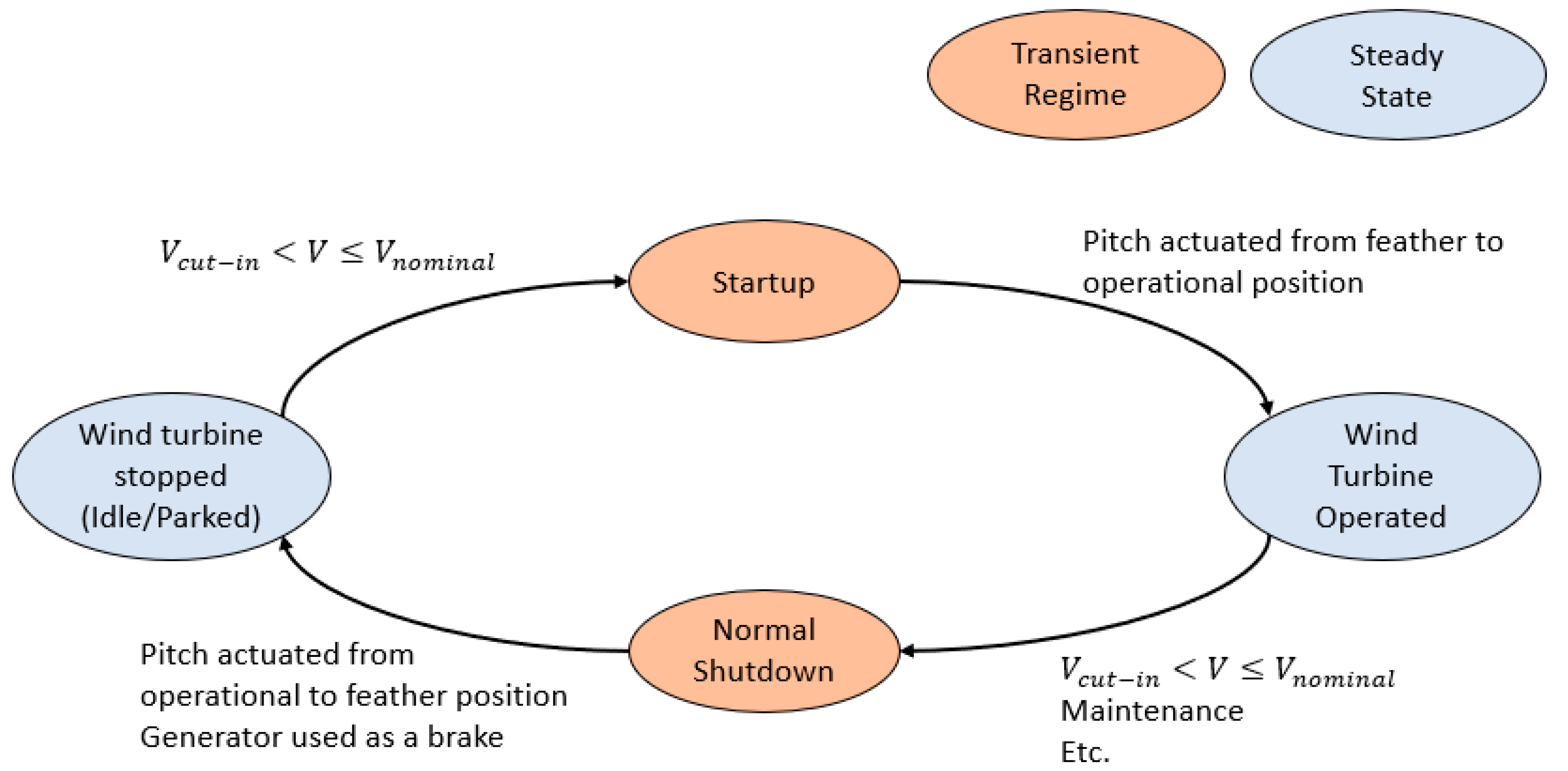
2.3. Operating Regimes

According to Hackl [39], WTs operate under four (4) regimes. Regime I represents a standstill condition due to insufficient wind ($V{\le V}_{cut-in}$), which results in no power output. Regime II entails variable power output corresponding to wind speed ($V_{cut-in}<V\le V_{nominal}$), followed by Regime III where power output remains at a nominal level regardless of wind speed ($V_{nominal}$ < WS < $V_{cut-out}$). Then, Regime IV is reached when the wind is excessive, causing the WT to return to a standstill state with no power output ($V_{cut-out}<V$).

However, this description has a limitation in that it only considers the standard operational conditions of the WT. In practice, for reasons related to maintenance or wind farm power output regulations, the WT may be kept in a stopped state even when there is sufficient wind for energy generation. If so, to maintain the WT in the stopped state, the turbine blades are pitched into a feathered position [27]. In such cases, aerodynamic forces differ from those during normal operation due to pitch angle variations [37,38,40]. Consequently, it can be assumed that the resulting fatigue damage is influenced by the operating regime.

In the present work, we preferred to categorize WT activities into two primary continuous regimes: Power Production and Parked. To transition between these continuous regimes, the WT undergoes transient regimes, namely, Start-up and Shutdown. These transient regimes impact WTB fatigue and are integral components of a reliable damage model [16,27,41]. In this study, power production and parked regimes are considered as continuous regimes when assessing fatigue damage, which is completed by adding damage induced by transient regimes. These transient regimes are subdivided into start-up and shutdown procedures and are summarized in Figure 1.

2.4. Hypothesis

Only the damage at the blade root location is investigated. The expectation is that the blade root section will be the WTB part most sensitive to fatigue damage [36,37,42,43]. The root section is considered circular, irrespective of the WTB structural design and the WT model considered [12,20,36,37,38], which limits the damage study to a simple shape. Moreover, the skin thickness and the diameter at the WTB root are influenced only by the overall WTB length [31,38,44]. This facilitates the configuration of a conceivable WTB root design from the numerical WTB model’s basic information. Variations of the stress induced by flapwise and edgewise bendings lead to the initiation and propagation of damage. Considering a WTB pitch with an angle $\alpha =0°$, the edgewise bending corresponds to the in-rotor plane direction while the flapwise bending is associated with the out-rotor plane direction. However, based on estimations carried out with a 5 MW WTB from the NREL library and the FAST simulation tool, the flapwise bending would seem to be more sensitive to WS fluctuations than the edgewise one. That is why this study focuses on the stress resulting from WS fluctuations. The simulated 1 Hz WS signal is stochastically generated via the FAST v8.16.00 TurbSim module, which uses the Kaimal spectrum [29]. In the literature, the Kaimal spectrum is often used to generate turbulent wind flows [45,46]. This spectrum was designed for a flat and homogenous onshore site [47]. Within the atmospheric boundary layer, using the Kaimal spectrum is one of the best ways to describe the turbulent wind field [48], and it is recommended by the IEC 61400 standard [24]. Finally, because damage is a cumulative phenomenon, it is assumed that the overall WTB damage $D_{\mathrm{T}\mathrm{o}\mathrm{t}}$ at time ($t\in {\mathbb{R}}_{+}$) is defined as a sum of many damages ($D_{\mathrm{i}}$), as follows:

$${\mathit{D}}_{\mathbf{T}\mathbf{o}\mathbf{t}}\left(\mathit{t}\right)={\mathit{D}}_{\mathbf{O}\mathbf{p}\mathbf{e}\mathbf{r}\mathbf{a}\mathbf{t}\mathbf{i}\mathbf{o}\mathbf{n}}\left(\mathit{t}\right)+{\mathit{D}}_{\mathbf{P}\mathbf{a}\mathbf{r}\mathbf{k}\mathbf{e}\mathbf{d}}\left(\mathit{t}\right)+{\mathit{D}}_{\mathbf{S}\mathbf{D}}\left(\mathit{t}\right)+{\mathit{D}}_{\mathbf{E}\mathbf{S}\mathbf{D}}\left(\mathit{t}\right)+{{\mathit{D}}_{\mathbf{S}\mathbf{U}}\left(\mathit{t}\right)+\mathit{D}}_{\mathbf{E}\mathbf{v}\mathbf{e}\mathbf{n}\mathbf{t}\mathbf{s}}\left(\mathit{t}\right)+{\mathit{D}}_{{\mathit{t}}_0}$$

(1)

Here, $D_{\mathrm{O}\mathrm{p}\mathrm{e}\mathrm{r}\mathrm{a}\mathrm{t}\mathrm{i}\mathrm{o}\mathrm{n}}$ is the damage induced by the operation of the WT, $D_{\mathrm{P}\mathrm{a}\mathrm{r}\mathrm{k}\mathrm{e}\mathrm{d}}\left(t\right)$ is the damage when the WT is stopped, and $D_{\mathrm{S}\mathrm{D}}$ and $D_{\mathrm{E}\mathrm{S}\mathrm{D}}$ are the damage during a normal WT shutdown and a WT emergency shutdown, respectively. $D_{\mathrm{S}\mathrm{U}}$ is the damage provoked by the WT start-up, and $D_{\mathrm{E}\mathrm{v}\mathrm{e}\mathrm{n}\mathrm{t}\mathrm{s}}$ represents the damage induced by extreme environmental conditions such as wind velocities higher than $V_{cut-out}$ (in our study, 25 m·s⁻¹), which can occur when a storm strikes the wind farm, for example. Finally, the initial damage occurring during the manufacturing process at time $t_0$ corresponds to $D_{t_0}$.

Because the damage induced by special environmental events involves complex mechanisms such as resonance problems or sudden material failures, as opposed to fatigue behavior [49], $D_{\mathrm{E}\mathrm{v}\mathrm{e}\mathrm{n}\mathrm{t}\mathrm{s}}$ is not considered in this study. Although it has been proven that $D_{t_0}$ can strongly impact the strength of the WTB [20,50,51], it is not considered in this study either, because $D_{t_0}$ is typically based on manufacturing defects, which are hard to assess and independent of the fatigue mechanism. It is therefore beyond the scope of this study, which focuses on damage induced by fatigue as a first step. Moreover, $D_{\mathrm{E}\mathrm{S}\mathrm{D}}$ is not considered herein because available SCADA data does not distinguish between emergency shutdowns and normal ones. Therefore, each shutdown is considered as normal. However, $D_{\mathrm{O}\mathrm{p}\mathrm{e}\mathrm{r}\mathrm{a}\mathrm{t}\mathrm{i}\mathrm{o}\mathrm{n}}$, $D_{\mathrm{P}\mathrm{a}\mathrm{r}\mathrm{k}\mathrm{e}\mathrm{d}}$, $D_{\mathrm{S}\mathrm{D}}$, and $D_{\mathrm{S}\mathrm{U}}$ are investigated because they rely on the fatigue behavior. The present work, for the first time, thus introduces a WTB fatigue damage assessment based on both 10-min aggregated SCADA data and the different WT operating regimes for a better comprehension of the damage evolution. The overall damage considered is presented in Equation (2):

$${\mathit{D}}_{\mathbf{T}\mathbf{o}\mathbf{t}}\left(\mathit{t}\right)={\mathit{D}}_{\mathbf{O}\mathbf{p}\mathbf{e}\mathbf{r}\mathbf{a}\mathbf{t}\mathbf{i}\mathbf{o}\mathbf{n}}\left(\mathit{t}\right)+{\mathit{D}}_{\mathbf{P}\mathbf{a}\mathbf{r}\mathbf{k}\mathbf{e}\mathbf{d}}\left(\mathit{t}\right)+{\mathit{D}}_{\mathbf{S}\mathbf{D}}\left(\mathit{t}\right)+{\mathit{D}}_{\mathbf{S}\mathbf{U}}\left(\mathit{t}\right)$$

(2)

3. Steady Regime Damage

3.1. Stress Assessment

The flapwise bending at the blade root ($M_{flap}$ [N·m]) as a function of WS was obtained by running the aeroelastic FAST software [40] in conjunction with a 5 MW WT numerical model from the NREL open access library (see Figure 2). Thereafter, it was possible to convert the WS history into a flapwise bending history, and then to convert the bending history into a stress history via Equation (3) (see Figure 3 and Figure 4).

$${\mathit{\sigma }}_{\mathit{f}\mathit{l}\mathit{a}\mathit{p}}=\frac{{\mathit{M}}_{\mathit{f}\mathit{l}\mathit{a}\mathit{p}}\mathit{c}}{\mathit{I}}$$

(3)

Here, ${\sigma }_{flap}$ is the resulting stress [Pa]. Then, $c$ [m] is defined as the maximum distance from the neutral axis, which is approximately equivalent to the chord line. Hence, at the WTB root, $c$ is barely equal to 50% of the airfoil thickness [m] [36,38] and $I$ represents the moment of inertia [m⁴] of the WTB root section.

The skin thickness of the WTB at the root $t_{root}$ [m] must be found in order to compute $I$. However, the $t_{root}$ corresponding to the numerical WTB used in this work is unknown. Moreover, the 5 MW WTB root thickness varies strongly as a function of the source (from 50 to 80 mm) [52,53,54]. As such, a reliable extrapolation of $t_{root}$ is difficult to process. Thus, following an empirical observation, $t_{root}$ was arbitrarily chosen [38]:

$${\mathit{t}}_{\mathit{r}\mathit{o}\mathit{o}\mathit{t}}\approx 0.08\sqrt{\frac{\mathit{R}}{40}}$$

(4)

Here, $R$ [m] corresponds to the rotor radius ($R=64$ m in this study).

Then, the RainFlow Counting (RFC) algorithm, as described in [55], was used to compute the characteristics of the stress cycles. The RFC considered the stress history and was undertaken in accordance with international standard recommendations [18,24]:

$$\left[\mathsf{\Delta }{\sigma }_i,n_i\right]=\mathrm{R}\mathrm{F}\mathrm{C}\left(u\left(t\right),\left|\sigma \right|,{\sigma }_u\right)$$

(5)

Here, $n_i$, is the cycle number according to $\mathsf{\Delta }{\sigma }_i$, the stress range amplitude of the cycles, and $i$ is the $i$-th stress cycle.

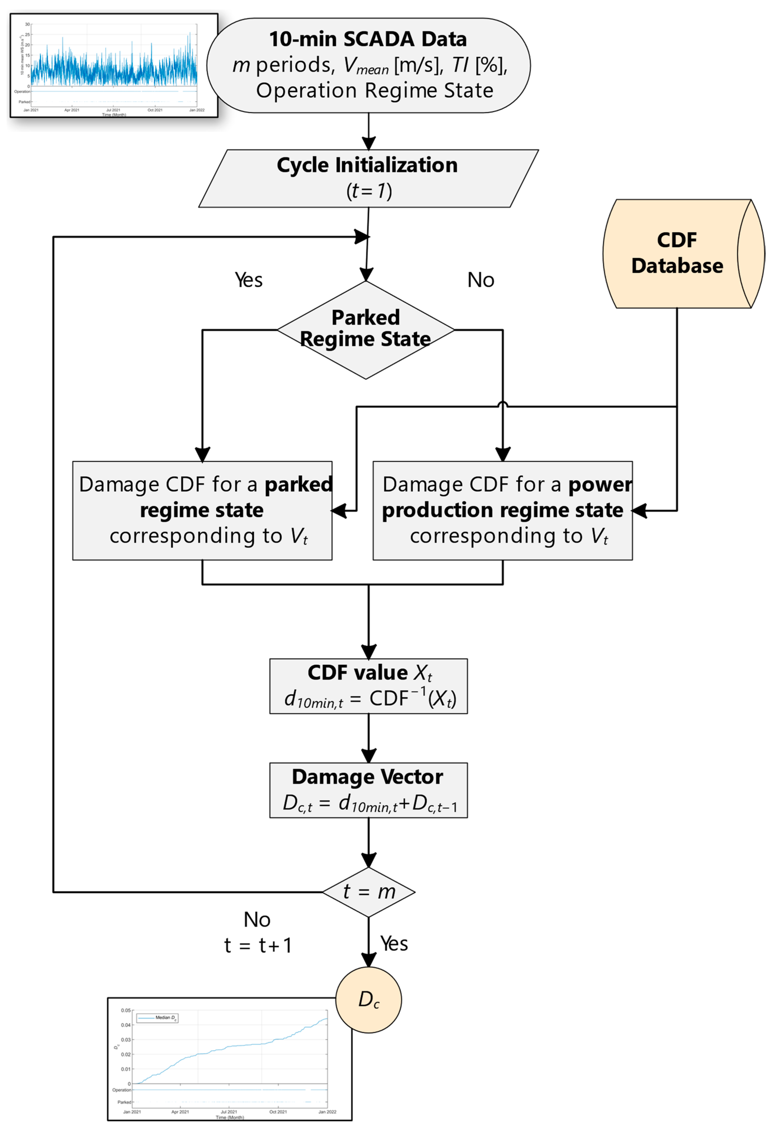
3.2. Assessment of Damage Based on 10-Min SCADA Data and 1 Hz Simulated WS Signal for Continuous Regimes

Working with the crude 10-min mean WS stored in the SCADA data is not enough for a WTB damage estimation, as it does not provide enough information about the WS fluctuation within the incoming wind flow. In fact, WTBs are sensitive to approximately 1 Hz WS fluctuations [31], so it is recommended to consider a WS signal with such a frequency in order to obtain a reliable WTB damage assessment [17]. To overcome the absence of 1 Hz WS history in the SCADA data, the method presented here therefore aims to compute the equivalent damage level for a simulated 1 Hz WS for a 10-min period, parametrized with a turbulence intensity and mean WS as defined by [17,56], given by the SCADA data:

$$TI=\frac{{\sigma }_V}{\overline{V}}$$

(6)

Here, $\overline{V}$ [m·s⁻¹] is the mean WS and ${\sigma }_V$ is the standard deviation characterizing the WS signal for a 10-min period.

To generate these 1 Hz wind speed signals, the method presented by [57] is used. The TurbSim module from FAST is run for a 10-min period to generate a series of 1 Hz WS signals [29]. The simulated WS profiles cover the entire spectrum of wind properties that the WT may encounter during its operating life, as defined by the IEC-61400-1 standard [24], in terms of $TI$ and mean WS. Multiple series of 10-min WS simulations at a 1 Hz frequency are thus carried out for $TI$ ranging from 1% to 50% and for mean WS going from 1 m·s⁻¹ to 30 m·s⁻¹. Moreover, each WS simulation series is composed of 100 10-min WS simulated signals (instead of six, which is the minimum required by the standard [24], to allow a better understanding of the damage distribution, explained later) (see Figure 5). The stochasticity and the turbulence of the WS signals are generated via the Kaimal spectrum, which is widely used in the WT industry and is recommended by the standards [18,24].

In the next step, the damage is computed for each of the 100 10-min simulated WS signals. For this damage calculation, the RFC of the stress resulting from the simulated WS is carried out using the method developed in Section 3.1. This done for the two continuous regimes (parked and power production) and the associated bending moment behaviors. While stress variations are commonly used in studies assessing WTB damage [13,14,15,17], when it comes to assessing damage in composite materials, [18] recommends using strain—rather than stress—variations. This is mainly because the different layers of a composite material maintain the same strain level when the laminate is subjected to a force, which is not the case with the stress level (see Figure 6). Thus, the RFC of the stress must be converted into an RFC of the strain. If the blade root layer stacking is known, the corresponding Young’s modulus of the material composing this WTB root can be computed [58]. Then, the RFC of the strain is obtained by converting the RFC of the stress using the Hooke’s law. This step provides $S_{i,A}$ and $S_{i,M}$ (respectively, the strain amplitude and mean strain) for each strain cycle i-th within a 10-min simulated WS. Using Equation (5), the strain RFC allows to compute the following:

$$\left[S_{i,A},n_i\right]=\mathrm{R}\mathrm{F}\mathrm{C}\left(u\left(t\right),S_{i,M},S_u\right)$$

(7)

Here, $S_u$ is taken as the maximum strain to failure of the weakest laminate ply.

To allow an assessment of the damage based on the computed strain history, an approach based on the Goodman diagram and the strain as proposed by DNV GL [18] was chosen. With this method, the number of cycles to failure $N_i$ for a strain cycle conditions i-th can be obtained via Equation (8):

$$N_i={\left[\frac{R_{i,t}+\left|R_{i,c}\right|-\left|2 {\gamma }_{Ma}{ S}_{i,M}-R_{i,t}+\left|R_{i,c}\right|\right|}{2 \left({\gamma }_{Mb}/C_{1b}\right) S_{i,A}}\right]}^m$$

(8)

with:

$${\gamma }_{Mb}/C_{1b}={\gamma }_{M0}{C}_{2b}{C}_{3b}{C}_{4b}{C}_{5b}$$

(9)

For presentation simplicity, all the parameters are presented in the Nomenclature.

Using the Miner’s rule as recommended by the standards [18,24], with $n_i$ being known thanks to the strain RFC, and $N_i$ given by Equation (8), the damage $d_{10min}$ for each WS signal can be computed:

$$d_{10\mathrm{m}\mathrm{i}\mathrm{n}}=\sum \frac{n_i}{N_i}$$

(10)

Following that, a database is built, and brings together $d_{HCF}$ for each 10-min mean WS and $TI$. Because WS series are composed of 100 WS signals, along with the corresponding wind parameters, a cumulative distribution function (CDF) of $d_{10\mathrm{m}\mathrm{i}\mathrm{n}}$ can be drawn for these specific parameters and as a function of the operating regime considered (see Figure 7 and Figure 8).

Finally, the global WTB damage induced by the continuous regimes $D_c$ can be computed by summing the corresponding damage $d_{10\mathrm{m}\mathrm{i}\mathrm{n},t}$ for each 10-min period in the SCADA data, considering the operating regime (power production or parked) at this moment (see Figure 9).

$$D_c=\sum _t{d}_{10\mathrm{m}\mathrm{i}\mathrm{n},t}$$

(11)

The process which allows the computation of $D_c$ is illustrated in Figure 10 and Figure 11. More details about the overall computation of $D_c$ are provided in the article written by [57].

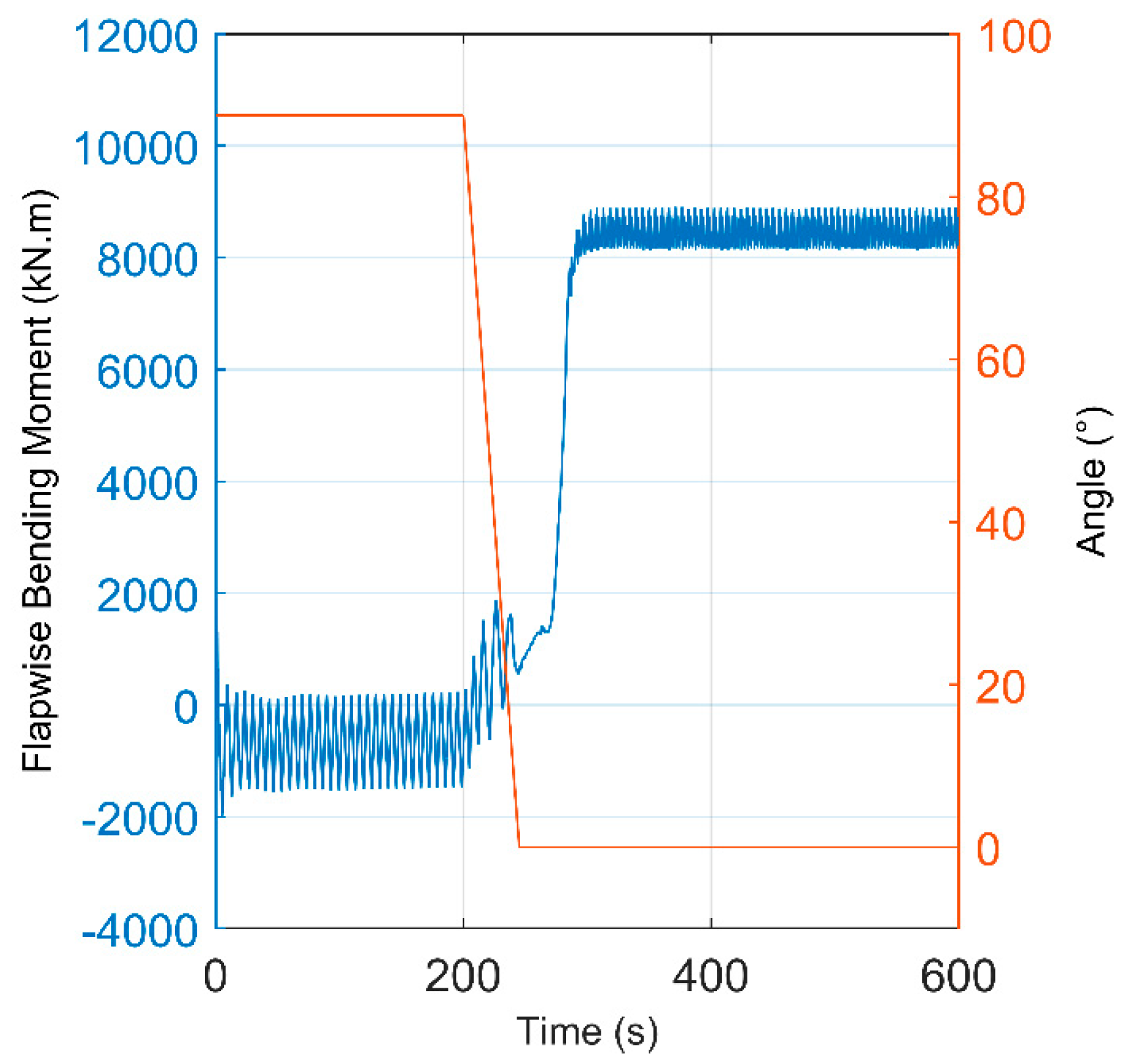
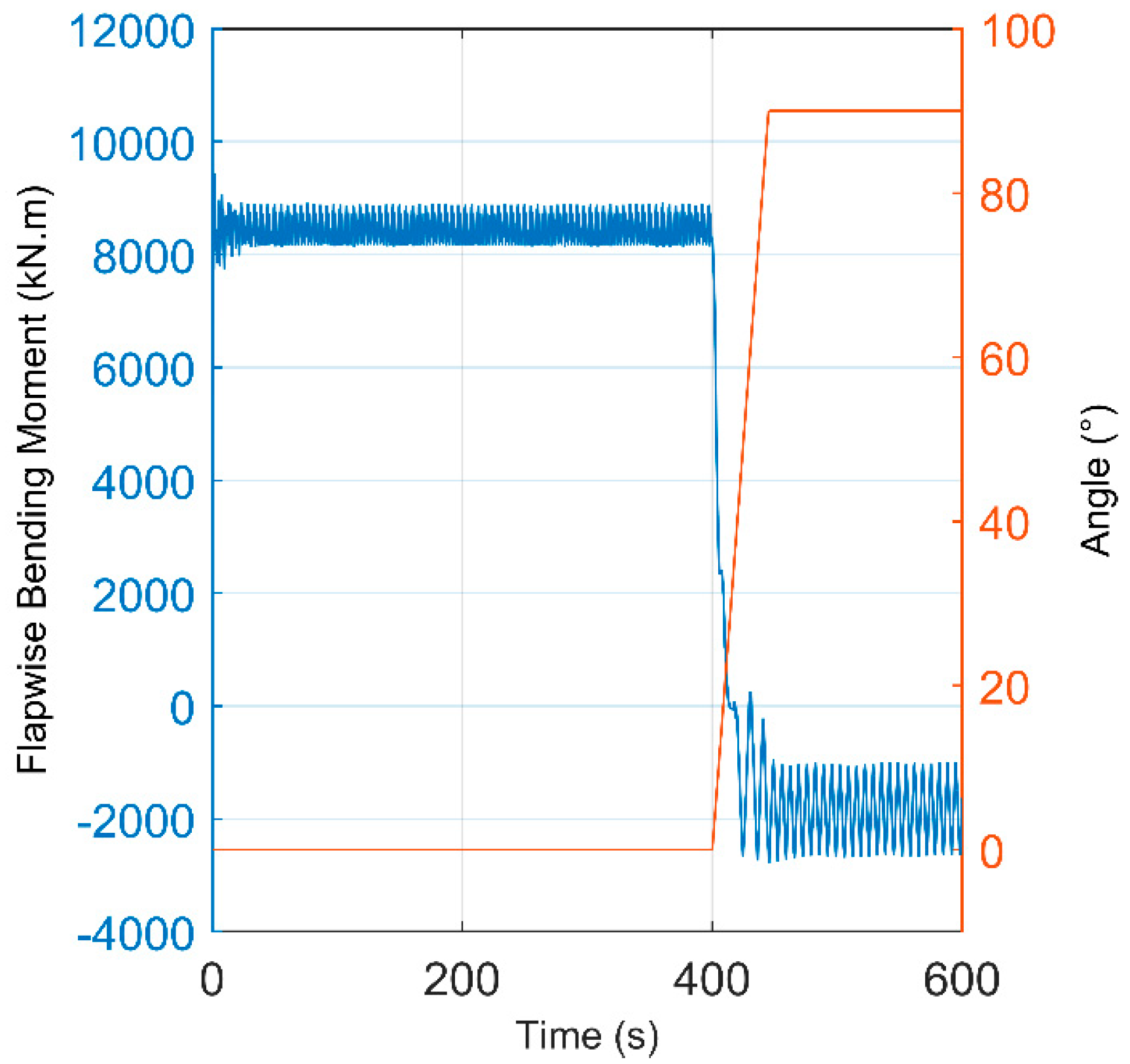
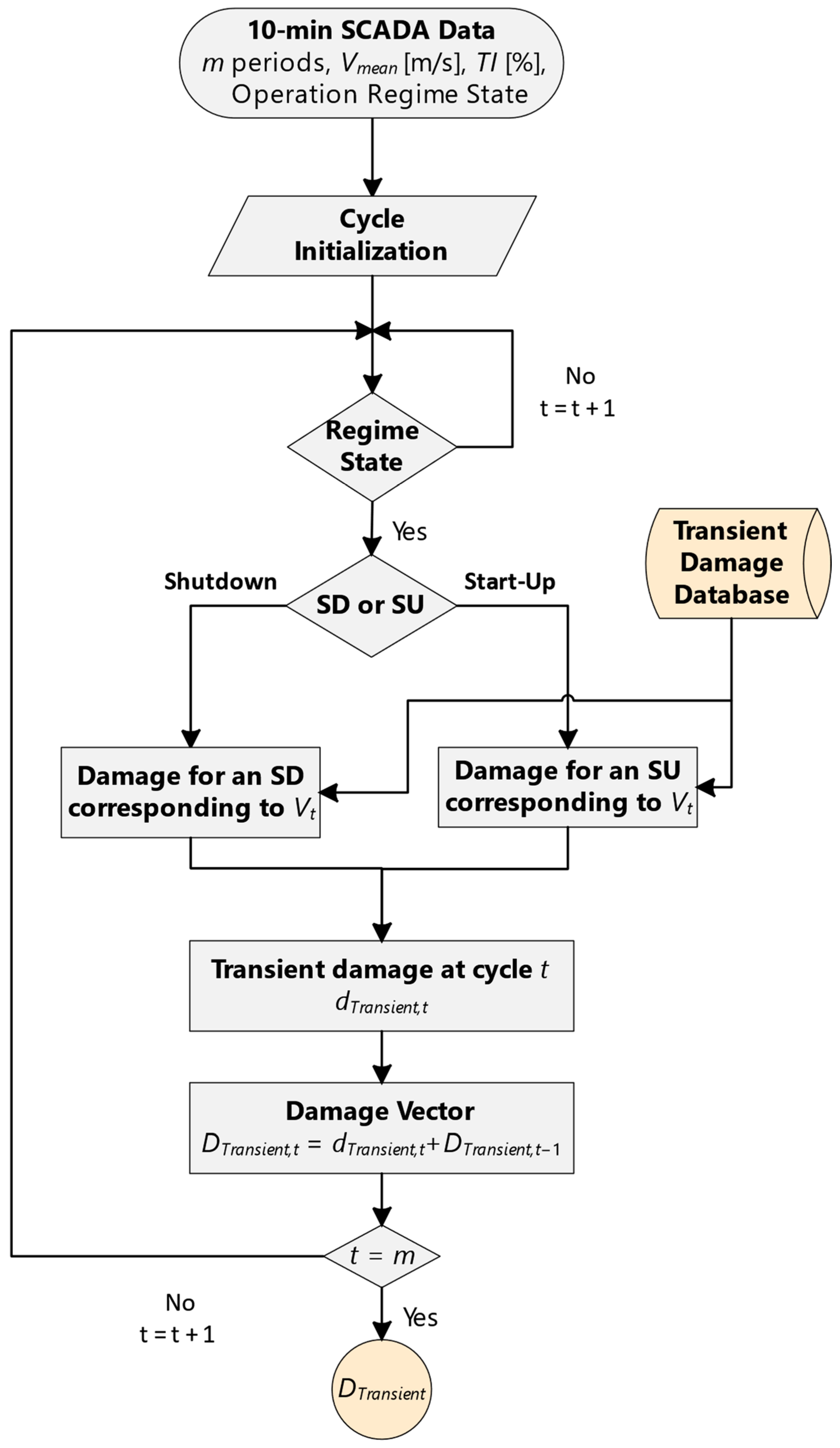
3.3. Assessment of the Damage Based on 10-Min SCADA Data and 1 Hz Simulated WS Signal for Transient Regimes

As depicted in Figure 1, proceeding from one continuous regime to another requires that the WT go through a transient regime (start-up or shutdown). According to the standards [18,24] and the scientific literature [16,27], the damage induced by such transient regimes must be taken into account. To compute the WTB damage induced by start-ups and shutdowns, these regimes are simulated using FAST and the start-up/shutdown procedure presented in the FAST user guide [40], in accordance with the IEC-61400-1 standard [24]. For pitch-regulated WT, the start-up is initiated by moving the blades from the feather position (pitch angle of 90°) to an operation position (between 90° and 0°) [16,18,24,27,37,40,59] and inversely so for the shutdown procedure. Throughout the simulation, the flapwise bending moment is directly computed by FAST, leading to a bending moment history. Within this history, the flapwise bending period induced by the transient regime procedure is arbitrarily delimited by the time period needed for the pitch angle to go from an initial position to a final one (see Figure 12 and Figure 13). Then, this flapwise bending history is converted into a strain history following the methodology presented in Section 3.1 and Section 3.2. Following that, the RFC is applied to the selected strain history to obtain the number of cycles $n_i$ at specific strain cycle conditions (in terms of mean strain and amplitude) and the number of cycles to failure $N_i$ at these specific strain cycle conditions is also computed via Equation (8). Finally, the damage induced by a transient regime is computed using the Miner’s rule, as described in Equation (10):

$${\mathit{d}}_{\mathit{t}\mathit{r}\mathit{a}\mathit{n}\mathit{s}\mathit{i}\mathit{e}\mathit{n}\mathit{t}}=\sum \frac{{\mathit{n}}_{\mathit{i}}}{{\mathit{N}}_{\mathit{i}}}$$

(12)

To get an overall idea of the damage due to transient regimes, start-ups and shutdowns are simulated for each mean WS ($V_{cut-in}<V\le V_{cut-out}$) and the damage is computed accordingly, leading to a transient damage database. Each time the SCADA data has registered a regime change at a certain mean WS, the corresponding transient damage $d_{transient}$ is selected and added to the global WTB damage estimation:

$${\mathit{D}}_{\mathit{T}\mathit{o}\mathit{t}}={\mathit{D}}_{\mathit{c}}+\sum _{\mathit{j}}{\mathit{d}}_{\mathit{t}\mathit{r}\mathit{a}\mathit{n}\mathit{s}\mathit{i}\mathit{e}\mathit{n}\mathit{t}}$$

(13)

Here, $j$ is the number of transient regimes. The process describing the transient damage computation is summarized in Figure 14.

4. Results and Discussion

Firstly, after a 4-year period, the evaluated global WTB damage $D_{\mathrm{T}\mathrm{o}\mathrm{t}}=1.85\times {10}^{-1}$. In other words, the WTB life expectancy is expected to be $21.6$ years if the 4-year period of study is reproduced till the failure of the WTB. This result is close to the normal $20$ years of life expectancy required by the standard IEC 61400-1 [24] and found in the literature even with different damage laws [10,11,60]. According to Equation (2), the global WTB damage can be decomposed as the sum of the damage induced by the power production, parked, and transient regimes. An analysis of the damage caused by these regimes was conducted and the findings are brought together in

Table 1. Distribution of global damage between the different wind turbine regimes.

Damage Category	Absolute Damage Value for a 4-Year Period	Percentage of Global Damage for a 4-Year Period
$D_{\mathrm{T}\mathrm{o}\mathrm{t}}$	$1.85\times {10}^{-1}$	$\mathrm{100\%}$
$D_{\mathrm{O}\mathrm{p}\mathrm{e}\mathrm{r}\mathrm{a}\mathrm{t}\mathrm{i}\mathrm{o}\mathrm{n}}$	$1.84\times {10}^{-1}$	$\mathrm{99.9\%}$
$D_{\mathrm{T}\mathrm{r}\mathrm{a}\mathrm{n}\mathrm{s}\mathrm{i}\mathrm{e}\mathrm{n}\mathrm{t}}$	$4.00\times {10}^{-6}$	<0.1%
$D_{\mathrm{P}\mathrm{a}\mathrm{r}\mathrm{k}\mathrm{e}\mathrm{d}}$	$4.48\times {10}^{-19}$	$\approx \mathrm{0\%}$

. Regarding these findings, it is evident that the main contributor to the total WTB damage, $D_{To\mathrm{t}}$, is the damage associated with the power production regime, $D_{Operation}$, over a 4-year period (as illustrated in Figure 15). Then, in terms of contribution significance to $D_{Tot}$ we have the damage induced by the transient regime $D_{Transient}$. Finally, $D_{\mathit{P}\mathit{a}\mathit{r}\mathit{k}\mathit{e}\mathit{d}}$ comes in last in the order of contribution to $D_{Tot}$. Compared to $D_{Tot}$, the value of $D_{Parked}$ is practically nil and could thus be neglected or replaced by a nil value.

If the WT is always considered as being in the power production regime, $D_{\mathrm{T}\mathrm{o}\mathrm{t}}$ may be overestimated by $\mathrm{3.8\%}$ in our case (see Figure 16). For $D_{\mathrm{T}\mathrm{r}\mathrm{a}\mathrm{n}\mathrm{s}\mathrm{i}\mathrm{e}\mathrm{n}\mathrm{t}}$, while it represents only a fraction of $D_{\mathrm{T}\mathrm{o}\mathrm{t}}$, it must be monitored for two main reasons. Firstly, its value directly depends on the number of start-ups and shutdowns of the WT. So, in the case of a WT with a larger number of start-ups/shutdowns, $D_{\mathrm{T}\mathrm{r}\mathrm{a}\mathrm{n}\mathrm{s}\mathrm{i}\mathrm{e}\mathrm{n}\mathrm{t}}$ could increase enough for its contribution to $D_{\mathrm{T}\mathrm{o}\mathrm{t}}$ to be non-negligeable. Secondly, $D_{\mathrm{T}\mathrm{r}\mathrm{a}\mathrm{n}\mathrm{s}\mathrm{i}\mathrm{e}\mathrm{n}\mathrm{t}}$ strongly depends on the wind speed at which the transient regimes occur (see Figure 17). If the transient regime surfaces at the nominal WS ($11 \mathrm{m}.{\mathrm{s}}^{-1}$ in our case), the corresponding damage will be much higher by far as compared to transient regimes operated at cut-in or cut-out WS ($4 \mathrm{m}·{\mathrm{s}}^{-1}$ and $25 \mathrm{m}·{\mathrm{s}}^{-1}$). This phenomenon is mainly explained by the fact that at $V_{nominal}$, the difference between the power production regime and the parked regime in terms of flapwise bending reaches its maximum, as shown in Figure 2.

This result is further corroborated by [16]. Therefore, if numerous transient regimes occur at the nominal WS, $D_{\mathrm{T}\mathrm{r}\mathrm{a}\mathrm{n}\mathrm{s}\mathrm{i}\mathrm{e}\mathrm{n}\mathrm{t}}$ will accordingly increase considerably. This result makes it essential to review the procedures for starting or stopping WT in order to avoid the transient regime at a nominal WS.

Finally, because $D_{\mathrm{O}\mathrm{p}\mathrm{e}\mathrm{r}\mathrm{a}\mathrm{t}\mathrm{i}\mathrm{o}\mathrm{n}}$ is the main contributor to $D_{\mathrm{T}\mathrm{o}\mathrm{t}},$ $D_{\mathrm{O}\mathrm{p}\mathrm{e}\mathrm{r}\mathrm{a}\mathrm{t}\mathrm{i}\mathrm{o}\mathrm{n}}$ is the priority target for the WTB useful life extension. As an example, by reducing the nominal power output, $D_{\mathrm{O}\mathrm{p}\mathrm{e}\mathrm{r}\mathrm{a}\mathrm{t}\mathrm{i}\mathrm{o}\mathrm{n}}$ would decrease, as would $D_{\mathrm{T}\mathrm{o}\mathrm{t}}$ [60], increasing the WTB RUL. Even if the nominal power decreases, an increase in total energy production can be expected thanks to the resulting extension of the RUL of the WTB, leading to an enhancement of financial profits for the WT operator. Therefore, the next step of this study will be to investigate the consequences of a nominal WT power reduction over the WTB RUL and energy production, helping the WT operator optimize its investments.

The algorithm used here has a time and space complexity of O(n). This enables rapid calculation of damage (2 s of computation time to assess one year of wind turbine damage from a home computer) over an extended period, which represents an improvement over the damage model proposed by [17] without altering the results due to the use of the same damage law. Furthermore, the proportion of damage generated by transient regimes compared to damage generated by the operating WT is found to be substantially similar to that found by [16], which reinforces the reliability of our results. Additionally, the presented method relies on SCADA data measured on-site, allowing for adaptation of this damage estimation procedure to the specific meteorological conditions of each WT. This makes it easier to adapt to different WT within the same wind farm than methods based on an exponential damage model, as proposed by [11]. Exponential models require shape and scale parameters that are difficult to obtain and need regular updating through WTB inspections, which we aim to avoid. The same applies to damage models based on dynamic Bayesian networks, where parameters are not transferable from one WT to another. Lastly, another advantage of the model presented here is that it allows for damage assessment from the wind turbine blade’s commissioning date, unlike methods based on the Paris law describing crack propagation. According to [12], a crack must preexist in the blade for the Paris law to be applicable. In other words, the wind turbine blade must already have sufficient damage for cracks to have appeared and thus for the Paris law to describe their propagation.

Regarding the drawbacks associated with this method, one can mention the lack of information on the design of the WTB used in the studied wind farm, as these are the private property of the manufacturer. This has led us to use a digital WTB model available in the NREL library as a basis for our work. Furthermore, in our study, we estimated the thickness of the blade at its root through an empirical formula, which also has its limitations, as it is only valid for WT designed to operate under a class A turbulence profile. Finally, there are also questions about the composite stratification at the root of the WTB. For now, all these uncertainties limit this method to providing a relative rather than absolute estimate of the RUL. The method thus only allows for comparing damage between similar WTs. To obtain absolute damage on a specific blade model, it would be necessary to calibrate this damage model with damage observed on turbines of the same type. Another drawback of this damage model is that it does not consider the impact of material degradation like delamination or cracks on WTB fatigue. Indeed, according to [61], blade damage can be expressed as the proportion of the effective surface area of the material capable of bearing loads compared to the same undamaged material as expressed below:

$$\mathit{D}=\frac{\mathit{A}-\tilde{\mathit{A}}}{\mathit{A}}$$

(14)

With $A$ being the damaged area and $\tilde{A}$ being the effective resisting area.

Consequently, as the blade becomes damaged, the effective stress $\tilde{\sigma }$ in the material will increase, as expressed below:

$$\tilde{\sigma }=\frac{\sigma }{1-D}$$

(15)

However, the damage model presented here does not consider this phenomenon, which may lead to an underestimation of the damage. So, this should be taken into account in future study to approach an absolute RUL evaluation.

5. Conclusions

The present work, for the first time, introduces a WTB fatigue damage evaluation based on both 10-min aggregated SCADA data and the different WT operating regimes (with operating and parked being continuous regimes, while start-up and shutdowns are grouped under the transient regimes class) for a better comprehension of the damage evolution. For this assessment, the global WTB fatigue damage was assumed to be the sum of the damage induced by the different regimes of operation. Firstly, starting with the RFC and the Miner’s rule, the WTB fatigue damage was computed for different load cases in terms of mean WS, $TI$ and operating regime conditions (power production, parked, start-up, and shutdown) for a 10-min period and with a WS sample frequency of 1 Hz. Then, the results were stored within a CDF database. Secondly, by reading the 10-min SCADA data history, the corresponding damage was selected from the CDF database and summed for the entire period of study. Via this method, a more comprehensive assessment of the WTB damage for a long period could be done, providing the WT operator with a decision-making tool which optimizes the maintenance schedule. However, this method requires calibration due to numerous uncertainties surrounding WTB damage, particularly related to assumptions about material properties and the blade root thickness. Consequently, the next step should calibrate the damage model to improve the damage estimation reliability.

Then, this study shows that the power production regime is by far the most contributing factor to the overall WTB fatigue damage compared to start-up/shutdown procedures and the parked regime. This conclusion underlines the importance of focusing on optimizing the power production regime to eventually protract the WTB RUL instead of investing efforts in improving start-up/shutdown procedures for limited results. This leads to understanding if it is possible to protract the WTB RUL by optimizing the power production regime. This is the subject of a future study.

References

1. DNV GL Energy Transition Outlook. DNV GL’s Energy Transition Outlook 2020. 2020. Available online: https://eto.dnvgl.com/2020/index.html (accessed on 4 December 2020).
2. Zhu, C.; Li, Y.; Zhu, C.; Li, Y. Reliability Analysis of Wind Turbines; IntechOpen: London, UK, 2018. [Google Scholar] [CrossRef]
3. Li, H.; Peng, W.; Huang, C.-G.; Guedes Soares, C. Failure Rate Assessment for Onshore and Floating Offshore Wind Turbines. JMSE 2022, 10, 1965. [Google Scholar] [CrossRef]
4. Mishnaevsky, L. Repair of wind turbine blades: Review of methods and related computational mechanics problems. Renew. Energy 2019, 140, 828–839. [Google Scholar] [CrossRef]
5. Technology Roadmap: Wind Energy 2013; IEA: Paris, France, 2013.
6. Ciang, C.C.; Lee, J.-R.; Bang, H.-J. Structural health monitoring for a wind turbine system: A review of damage detection methods. Meas. Sci. Technol. 2008, 19, 122001. [Google Scholar] [CrossRef]
7. Almond, D.P.; Avdelidis, N.P.; Bendada, H.; Ibarra-Castanedo, C.; Maldague, X.; Kenny, S. Structural Integrity Assessment of Materials by Thermography. In Proceedings of the Conference on Damage in Composite Materials, Stuttgart, Germany, 18–19 September 2006. [Google Scholar]
8. Sørensen, B.F.; Lading, L.; Sendrup, P.; McGugan, M.; Debel, C.P.; Kristensen, O.J.D.; Larsen, G.C.; Hansen, A.M.; Rheinländer, J.; Rusborg, J.; et al. Fundamentals for Remote Structural Health Monitoring of Wind Turbine Blades—A Pre-Project; Risø National Laboratory: Roskilde, Denmark, 2002. [Google Scholar]
9. Jørgensen, E.R.; Borum, K.K.; McGugan, M.; Thomsen, C.L.; Jensen, F.M. Full Scale Testing of Wind Turbine Blade to Failure—Flapwise Loading; U.S. Department of Energy: Oak Ridge, TN, USA, 2004. [Google Scholar]
10. Nielsen, J.S.; Sørensen, J.D. Bayesian Estimation of Remaining Useful Life for Wind Turbine Blades. Energies 2017, 10, 664. [Google Scholar] [CrossRef]
11. Asgarpour, M.; Sørensen, J.D. Bayesian based Prognostic Model for Predictive Maintenance of Offshore Wind Farms. Int. J. Progn. Health Manag. 2018, 9, 10. [Google Scholar] [CrossRef]
12. Eder, M.A.; Chen, X. FASTIGUE: A computationally efficient approach for simulating discrete fatigue crack growth in large-scale structures. Eng. Fract. Mech. 2020, 233, 107075. [Google Scholar] [CrossRef]
13. Liu, P.F.; Chen, H.Y.; Wu, T.; Liu, J.W.; Leng, J.X.; Wang, C.Z.; Jiao, L. Fatigue Life Evaluation of Offshore Composite Wind Turbine Blades at Zhoushan Islands of China Using Wind Site Data. Appl. Compos. Mater. 2023, 30, 1097–1122. [Google Scholar] [CrossRef]
14. Chen, Y.; Wu, D.; Li, H.; Gao, W. Quantifying the fatigue life of wind turbines in cyclone-prone regions. Appl. Math. Model. 2022, 110, 455–474. [Google Scholar] [CrossRef]
15. Sanchez, H.; Sankararaman, S.; Escobet, T.; Puig, V.; Frost, S.; Goebel, K. Analysis of two modeling approaches for fatigue estimation and remaining useful life predictions of wind turbine blades. In Proceedings of the PHM Society European Conference, Bilbao, Spain, 5–8 July 2016; Volume 11. [Google Scholar]
16. Jiang, Z.; Moan, T.; Gao, Z. A Comparative Study of Shutdown Procedures on the Dynamic Responses of Wind Turbines. J. Offshore Mech. Arct. Eng. 2015, 137, 011904. [Google Scholar] [CrossRef]
17. Jang, Y.J.; Choi, C.W.; Lee, J.H.; Kang, K.W. Development of fatigue life prediction method and effect of 10-minute mean wind speed distribution on fatigue life of small wind turbine composite blade. Renew. Energy 2015, 79, 187–198. [Google Scholar] [CrossRef]
18. Germanischer Lloyd. Guideline for the Certification of Wind Turbine; Germanischer Lloyd: Hamburg, Germany, 2010; Volume 384. [Google Scholar]
19. Bergami, L.; Gaunaa, M. Analysis of aeroelastic loads and their contributions to fatigue damage. J. Phys Conf. Ser. 2014, 555, 012007. [Google Scholar] [CrossRef]
20. Marín, J.C.; Barroso, A.; París, F.; Cañas, J. Study of fatigue damage in wind turbine blades. Eng. Fail. Anal. 2009, 16, 656–668. [Google Scholar] [CrossRef]
21. Vera-Tudela, L.; Kühn, M. Analysing wind turbine fatigue load prediction: The impact of wind farm flow conditions. Renew. Energy 2017, 107, 352–360. [Google Scholar] [CrossRef]
22. Tibaldi, C.; Henriksen, L.C.; Hansen, M.H.; Bak, C. Wind turbine fatigue damage evaluation based on a linear model and a spectral method: Wind turbine fatigue damage evaluation. Wind. Energy 2016, 19, 1289–1306. [Google Scholar] [CrossRef]
23. Ragan, P.; Manuel, L. Comparing Estimates of Wind Turbine Fatigue Loads Using Time-Domain and Spectral Methods. Wind. Eng. 2007, 31, 83–99. [Google Scholar] [CrossRef]
24. IEC 61400-1; Wind Turbines Part 1: Design Requirements. International Electrotechnical Commission: London, UK, 2005.
25. Valeti, B.; Pakzad, S.N. Estimation of Remaining Useful Life of a Fatigue Damaged Wind Turbine Blade with Particle Filters. In Dynamics of Civil Structures; Pakzad, S., Ed.; Springer International Publishing: Cham, Switzerland, 2019; Volume 2, pp. 319–328. [Google Scholar] [CrossRef]
26. IEC 61400-12-1 Ed. 2.0 b:2017; Wind Energy Generation Systems—Part 12-1: Power Performance Measurements of Electricity Producing Wind Turbines. International Electrotechnical Commission: London, UK, 2017.
27. Jiang, Z.; Xing, Y. Load mitigation method for wind turbines during emergency shutdowns. Renew. Energy 2022, 185, 978–995. [Google Scholar] [CrossRef]
28. Kaimal, J.C.; Wyngaard, J.C.J.; Izumi, Y.; Coté, O.R. Spectral characteristics of surface-layer turbulence. Q. J. R. Meteorol. Soc. 1972, 98, 563–589. [Google Scholar]
29. Jonkman, B.J.; Buhl, M.L. TurbSim User’s Guide; Technical Report; National Renewable Energy Lab. (NREL): Golden, CO, USA, 2006. [Google Scholar]
30. POWER|Data Access Viewer. Available online: https://power.larc.nasa.gov/data-access-viewer/ (accessed on 8 February 2024).
31. Dykes, K.L.; Rinker, J. WindPACT Reference Wind Turbines; National Renewable Energy Lab. (NREL): Golden, CO, USA, 2018. [Google Scholar] [CrossRef]
32. Jonkman, J.; Butterfield, S.; Musial, W.; Scott, G. Definition of a 5-MW Reference Wind Turbine for Offshore System Development; National Renewable Energy Lab. (NREL): Golden, CO, USA, 2009. [Google Scholar] [CrossRef]
33. Hawileh, R.A.; Abu-Obeidah, A.; Abdalla, J.A.; Al-Tamimi, A. Temperature effect on the mechanical properties of carbon, glass and carbon–glass FRP laminates. Constr. Build. Mater. 2015, 75, 342–348. [Google Scholar] [CrossRef]
34. Hu, W.; Chen, W.; Wang, X.; Jiang, Z.; Wang, Y.; Verma, A.S.; Teuwen, J.J. A computational framework for coating fatigue analysis of wind turbine blades due to rain erosion. Renew. Energy 2021, 170, 236–250. [Google Scholar] [CrossRef]
35. Barnes, R.H.; Morozov, E.V.; Shankar, K. Improved methodology for design of low wind speed specific wind turbine blades. Compos. Struct. 2015, 119, 677–684. [Google Scholar] [CrossRef]
36. Damkilde, L.; Larsen, T.J.; Walbjørn, J.; Sørensen, J.D.; Kirt, R.; Plauborg, J.; Lübbert, M.; Karatzas, V. Wind Turbine Blades Handbook; Bladena: Copenhagen, Danemark, 2017. [Google Scholar]
37. Manwell, J.F.; McGowan, J.G.; Rogers, A.L. Wind Energy Explained; John Wiley & Sons: Hoboken, NJ, USA, 2009. [Google Scholar]
38. Joncas, S. Thermoplastic Composite Wind Turbine Blades. Ph.D. Thesis, TU Delft Library, Delft, The Netherlands, 2010. [Google Scholar]
39. Hackl, C.M. Funnel control for wind turbine systems. In Proceedings of the 2014 IEEE Conference on Control Applications (CCA), Juan Les Antibes, France, 8–10 October 2014; pp. 1377–1382. [Google Scholar] [CrossRef]
40. Jonkman, J.M.; Buhl, M.L., Jr. FAST User’s Guide—Updated August 2005; National Renewable Energy Lab. (NREL): Golden, CO, USA, 2005. [Google Scholar] [CrossRef]
41. Luan, C.; Moan, T. On Short-Term Fatigue Analysis for Wind Turbine Tower of Two Semi-Submersible Wind Turbines Including Effect of Startup and Shutdown Processes. J. Offshore Mech. Arct. Eng. 2021, 143, 012003. [Google Scholar] [CrossRef]
42. Zárate-Miñano, R.; Anghel, M.; Milano, F. Continuous wind speed models based on stochastic differential equations. Appl. Energy 2013, 104, 42–49. [Google Scholar] [CrossRef]
43. Kong, C.; Kim, T.; Han, D.; Sugiyama, Y. Investigation of fatigue life for a medium scale composite wind turbine blade. Int. J. Fatigue 2006, 28, 1382–1388. [Google Scholar] [CrossRef]
44. Bortolotti, P.; Tarres, H.C.; Dykes, K.L.; Merz, K.; Sethuraman, L.; Verelst, D.; Zahle, F. IEA Wind TCP Task 37: Systems Engineering in Wind Energy—WP2.1 Reference Wind Turbines; National Renewable Energy Lab. (NREL): Golden, CO, USA, 2019. [Google Scholar]
45. Yi, W.; Lu, Z.; Hao, J.; Zhang, X.; Chen, Y.; Huang, Z. A Spectrum Correction Method Based on Optimizing Turbulence Intensity. Appl. Sci. 2021, 12, 66. [Google Scholar] [CrossRef]
46. Hong, X.; Li, J. Stochastic Fourier spectrum model and probabilistic information analysis for wind speed process. J. Wind. Eng. Ind. Aerodyn. 2018, 174, 424–436. [Google Scholar] [CrossRef]
47. Cheynet, E.; Jakobsen, J.B.; Obhrai, C. Spectral characteristics of surface-layer turbulence in the North Sea. Energy Procedia 2017, 137, 414–427. [Google Scholar] [CrossRef]
48. Couche Limite Atmosphérique—Centre National de Recherches Météorologiques. Available online: https://www.umr-cnrm.fr/spip.php?rubrique186 (accessed on 6 March 2023).
49. Chou, J.-S.; Chiu, C.-K.; Huang, I.-K.; Chi, K.-N. Failure analysis of wind turbine blade under critical wind loads. Eng. Fail. Anal. 2013, 27, 99–118. [Google Scholar] [CrossRef]
50. Li, J.; Wang, J.; Zhang, L.; Huang, X.; Yu, Y. Study on the Effect of Different Delamination Defects on Buckling Behavior of Spar Cap in Wind Turbine Blade. Adv. Mater. Sci. Eng. 2020, 2020, 6979636. [Google Scholar] [CrossRef]
51. Murdy, P.; Hughes, S.; Barnes, D. Characterization and repair of core gap manufacturing defects for wind turbine blades. J. Sandw. Struct. Mater. 2022, 24, 2083–2100. [Google Scholar] [CrossRef]
52. Sun, Z.; Sessarego, M.; Chen, J.; Shen, W.Z. Design of the OffWindChina 5 MW Wind Turbine Rotor. Energies 2017, 10, 777. [Google Scholar] [CrossRef]
53. Hiebel, M.; Schlipf, D. Case Study: D50 Offshore Wind Turbine; Aerodyn Engineering: Puchong, Malaysia, 2018. [Google Scholar]
54. We Are LM Wind Power—The Leading Rotor Blade Supplier to the Wind Industry|LM Wind Power. Available online: https://www.lmwindpower.com/ (accessed on 8 March 2023).
55. Rainflow Counts for Fatigue Analysis—MATLAB Rainflow. Available online: https://www.mathworks.com/help/signal/ref/rainflow.html?searchHighlight=C#d123e146736 (accessed on 13 April 2022).
56. Kim, D.-Y.; Kim, Y.-H.; Kim, B.-S. Changes in wind turbine power characteristics and annual energy production due to atmospheric stability, turbulence intensity, and wind shear. Energy 2021, 214, 119051. [Google Scholar] [CrossRef]
57. Chrétien, A.; Tahan, A.; Cambron, P.; Oliveira-Filho, A. Operational Wind Turbine Blade Damage Evaluation Based on 10-min SCADA and 1 Hz Data. Energies 2023, 16, 3156. [Google Scholar] [CrossRef]
58. Kollar, L.P.; Springer, G.S. Mechanics of Composite Structures; Cambridge University Press: Cambridge, UK; New York, NY, USA, 2003. [Google Scholar]
59. Pape, M.; Kazerani, M. Turbine Startup and Shutdown in Wind Farms Featuring Partial Power Processing Converters. IEEE Open Access J. Power Energy 2020, 7, 254–264. [Google Scholar] [CrossRef]
60. Requate, N.; Meyer, T.; Hofmann, R. From wind conditions to operational strategy: Optimal planning of wind turbine damage progression over its lifetime. Dynamics and control/Wind turbine control. Wind. Energy Sci. Discuss. 2022, 8, 1727–1753. [Google Scholar] [CrossRef]
61. Movaghghar, A.; Lvov, G.I. A Method of Estimating Wind Turbine Blade Fatigue Life and Damage using Continuum Damage Mechanics. Int. J. Damage Mech. 2012, 21, 810–821. [Google Scholar] [CrossRef]
Figure 1. Schema showing the normal regime cycle of a WT during its operating life. The conditions initiating the transient regimes and the activated WT parts enabling this transition are specified.
Energies 17 01202 g001
Figure 2. Graphic showing the behavior of the mean flapwise bending moment according to the wind speed in parked and operating regimes.
Energies 17 01202 g002
Figure 3. Example of a SCADA 10-min mean wind speed history over a 1-month period.
Energies 17 01202 g003
Figure 4. Computed flapwise bending moment for a 10-min SCADA data mean wind speed history over a 1-month period.
Energies 17 01202 g004
Figure 5. Simulation of 100 stochastic WS signals with V ¯ = 12   m · s 1 and T I = 13% for a period of 10 min.
Energies 17 01202 g005
Figure 6. Schema illustrating the stress and strain behavior within a laminate subjected to solicitations.
Energies 17 01202 g006
Figure 7. d 10 m i n CDF for V ¯ = 12   m · s 1 and T I = 13% corresponding to the WS profiles generated in Figure 5 for a 5 MW WT in power production state regime.
Energies 17 01202 g007
Figure 8. d 10 m i n CDF for V ¯ = 12   m · s 1 and T I = 13% corresponding to the WS profiles generated in Figure 5 for a 5 MW WT in parked state regime.
Energies 17 01202 g008
Figure 9. Computed damage D c through time with the corresponding operating regime history.
Energies 17 01202 g009
Figure 10. Flowchart showing the process leading to the construction of the CDF database of d 10 m i n .
Energies 17 01202 g010
Figure 11. Flowchart showing the process leading to the estimation of D c from the SCADA data.
Energies 17 01202 g011
Figure 12. Flapwise bending moment and pitch angle for a simulated start-up procedure from an idle state with V ¯ = 10   m · s 1 .
Energies 17 01202 g012
Figure 13. Flapwise bending moment and pitch angle for a simulated shutdown procedure to an idle state with V ¯ = 10   m · s 1 .
Energies 17 01202 g013
Figure 14. Flowchart showing the process leading to the estimation of D t r a n s i e n t from SCADA data.
Energies 17 01202 g014
Figure 15. Graph showing D O p e r a t i o n according to the time and the regime state history.
Energies 17 01202 g015
Figure 16. Graph comparing the computed WTB damage for a WT firstly evaluated as always in the power production regime only, with a more detailed damage assessment for the same WT, this time encompassing both continuous and transient regimes over a one-year period.
Energies 17 01202 g016
Figure 17. Graph showing D T r a n s i e n t according to the time and the regime states history. A graph of D T r a n s i e n t according to the wind speed has been added to better understand that sudden damage increases occur when transient regimes are operated near the nominal WS of the WT (11 m·s−1 in our case).
Energies 17 01202 g017