Article

Residual Life Prediction of Low-Voltage Circuit Breaker Thermal Trip Based on the Wiener Process

1
Provincial and Ministerial Co-Construction Collaborative Innovation Center on Reliability Technology of Electrical Products, Hebei University of Technology, Tianjin 300130, China
2
Key Laboratory of Electromagnetic Field and Electrical Appliance Reliability of Hebei Province, Hebei University of Technology, Tianjin 300130, China
*
Author to whom correspondence should be addressed.
Energies 2024, 17(5), 1189; https://doi.org/10.3390/en17051189
Submission received: 18 January 2024 / Revised: 22 February 2024 / Accepted: 27 February 2024 / Published: 1 March 2024
(This article belongs to the Section J: Thermal Management)

Abstract

:
A low-voltage circuit breaker thermal trip plays a role in power systems, including opening and closing, control, protection, and more. Their reliability directly affects the security and stability of the power distribution system. The Wiener process model is established according to the accelerated degradation data of thermal trips, and remaining life prediction is carried out. In this paper, firstly, the constant stress accelerated degradation test is carried out on a thermal trip with temperature as the accelerated stress and specific thermal deflection as the degradation eigenquantity to characterise the degradation trajectory according to the degradation data and analyse the degradation law; then, it is verified by the test of normal distribution that the degradation data of the thermal trip conform to the Wiener process. The Wiener process, using the great likelihood estimation method to estimate the parameters of the remaining life, calculates the remaining life probability density function and reliability function under different temperature stresses and obtains the remaining life of the thermal trip under each accelerated stress conditions; finally, the remaining life of the thermal trip at the initial moment is taken as the pseudo-failure life, and the Arrhenius accelerated model is utilised to launch the external thermal trip under normal stress. Finally, the Arrhenius acceleration model is used to extrapolate the lifespan of the thermal trip under normal stress.

1. Introduction

Low-voltage circuit breakers are mainly used for power distribution system disconnection, control, protection, and closure control, as well as the protection of common line faults and equipment faults. A thermal trip is an important part of the low-voltage circuit breaker. In the line, equipment overload faults that occur in the circuit breaker will produce a large amount of heat. The change in temperature will cause the elastic deformation of its action element, thermal bimetal. The thermal bimetal drives the operation by sensing the temperature change to realise overload protection, but the long-term high temperature will increase the thermal sensitivity of the bimetal, affecting the reliability and life of the thermal trip, and it cannot be effectively protected, which will cause serious economic losses and even jeopardise the safety of people [1,2]. Therefore, it is of great significance to analyse the performance degradation of thermal trips and predict the remaining life of thermal trips to ensure the safe operation of low-voltage distribution systems and the stable work of electric equipment.
Currently, residual life prediction and reliability assessment are widely used in various industries such as low-voltage electrical appliances [3,4]. Most of the current research focuses on assessment prediction based on methods such as neural networks, the Wiener process, the Gamma process, and support vector machines. Li et al. similarly used overtravel time as a degradation feature quantity of relay, improved wavelet packet transform, and combined it with a radial basis function neural network model to predict the life of the relay [5]; Liu et al. proposed a reliability assessment method based on an improved Bootstrap-Bayes procedure for electronic residual-current-operated circuit breakers and used a grey GM(1, 1) model for test data. The grey GM(1, 1) model was used to expand the test data as a priori information, and the parameter estimates were obtained through Gibbs sampling in the Markov chain Monte Carlo algorithm combined with the Bayes formula. The reliability assessment of the residual-current-operated circuit breaker under the normal use environment was achieved through the accelerated model of Arrhenius [6].
Feng Hailin et al. aimed to address the issue of low accuracy in the assessment of degraded products’ reliability when dealing with small sample sizes. They modelled the degradation trajectory of the product’s performance based on the nature of SVR and updated the model parameters combined with the Bayes theory, considering the availability of historical life data for the same batch of products, to obtain the reliability analysis of the product’s lifespan [7]. Zhang Zherui et al. selected the maximum arc ignition voltage and contact resistance as the characteristic parameters to be preferred, which were constructed as health indicators through numerical modelling, and then established a data-driven model for the remaining service life of the contactor based on the health indicators by using a BP neural network [8]. Li Kui et al. used the contact mass loss of an AC contactor as the performance degradation parameter and employed statistical regression methods, along with a nonlinear Wiener degradation model, to develop a prediction model for the contact mass loss of an AC contactor. This allowed for the estimation of the remaining life of the AC contactor [9]. Chen L et al. utilised a sliding-window grey model and a particle filter to improve the accuracy of predicting the remaining life of a battery when there is inadequate data available. A new life prediction model was constructed [10]. Li Xiaobei et al. chose the cumulative arc energy and suction time as the main input parameters of the prediction model and optimised the BP neural network model by a genetic algorithm. The test data of different test specimens were used as the training samples and validation samples, respectively, for the prediction, with the maximum prediction error being less than 11% [11]. Zhang Lijie et al. proposed a multi-objective optimisation method for a constant-stress-accelerated ageing test based on the Gamma process and validated the method by using the test data of carbon film resistors [12].
In this paper, the thermally sensitive performance ratio bending K of the thermal trip bimetal is selected as the degradation characteristic value. Temperature is taken as the accelerating variable to carry out the constant-stress-accelerated degradation test. Moreover, a Wiener-based degradation model is established, and the maximum likelihood estimation method is used to estimate the parameters of the model to predict its remaining service life under accelerated stress. Finally, the Arrhenius accelerated model is employed externally to determine the service life of a thermal trip under normal operation.

2. Accelerated Degradation Test for Thermal Trip

2.1. Acceleration Modelling and Determination of Acceleration Stresses

Low-voltage circuit breakers are mainly affected by temperature, humidity, vibration, sand, dust, salt spray, and other factors during actual use. According to BS EN 60947-2:2016 [13] and the product instruction manual, to ensure safe use of the product, the low-voltage circuit breakers are typically installed in a fixed manner and without any noticeable vibration during installation. Therefore, under normal use conditions, the vibration factor can be ignored. The working principle of the thermal cut-out relies on the thermal effect of the current to achieve protection, and the thermal cut-out is in a relatively enclosed space inside the circuit breaker, so the influence of other factors on the thermal cut-out can be ignored. The temperature is the main factor affecting the performance of the thermal cut-out, so the accelerated degradation test model for the thermal cut-out is selected from the Arrhenius model, and the temperature is taken as the accelerating stress for the test.
The Arrhenius model is a model that describes the relationship between the rate of a chemical reaction and temperature at a given temperature and is widely used and well established. It describes the rate of degradation of a product as being inversely proportional to the exponential function of the activation energy divided by temperature and Boltzmann’s constant. Its expression is as follows:
d M d t = A e E K T
where d M d t is the chemical reaction rate; A is a constant; E is the activation energy, representing the energy required for molecular diffusion and the binding surface of the active and passive layers of the hot bimetal sheet at high temperatures; K is Boltzmann’s constant; and T is the absolute temperature. Equation (1) is known as the Arrhenius equation, and the integration of both sides of Equation (1) (from 0 to t) leads to the following:
M 0 M d M = 0 t A e E K T d t
If the temperature T is a constant, then
M M 0 = A e E K T t
Let Δ M = M M , then t = Δ M A e E K T ; taking logarithms on both sides of Equation (3) yields
lg t = lg Δ M A + E K T lg e
Let a = lg Δ M A , b = E K lg e ; then, Equation (4) can be written as
lg t = a + b T
where t is the lifetime of the product, and the logarithm of the product lifetime t is linearly related to the inverse of the temperature T.

2.2. Determination of Test Parameters

According to the national standard GB/14048.2-2020 [14], it can be seen that the circuit breaker used in this paper needs to meet the thermal conditions of 1.3 in 1 h to pass into the debuckling, when in this condition 1 h just to debuckle, the value of the specific thermal deflection K that is obtained for the failure threshold. The thrust force generated by the bimetal required for the thermal trip to decouple was obtained through decoupling experiments to be 4.0 N, and the deflection of the bimetal was 2.2 mm. Through simulation analysis, the size of the specific thermal deflection K value is constantly changed, so that the bimetal deflection f = 2.2 mm during the specified time of decoupling, and the decoupling force F = 4 N can be regarded as being in the failure criticality, and at this time, the specific thermal deflection K ≤ 13.6 × 10⁻⁶/°C. There is also a certain difference between the initial specific thermal deflection of the thermal trip. Therefore, the failure threshold selected for the accelerated degradation test of the thermal trip is the relative failure threshold, and if the initial value of the specific thermal deflection K of the thermal trip is Q, then according to the theory of Wiener’s degradation model, the failure threshold of the thermal trip can be set as L = Q − 13.6 × 10⁻⁶/°C.
The stabilising temperature of the bimetal during the operation of a low-voltage circuit-breaker at a rated current is about 70 °C, and the minimum stress level is selected to be 90 °C for T1. In the temperature range from room temperature to 200 °C, the maximum load stress without residual thermal deformation and permanent deformation of the thermal bimetal, the core element of overload protection, is about σ max = 200 MPa. Therefore, the bimetal’s maximum allowable temperature rises. Formula (6) can be derived from the initial temperature of 25 °C; the bimetal does not produce residual thermal deformation or permanent deformation at the temperature of 125 °C, leaving a certain safety margin. The upper limit of the temperature can be taken as 120 °C.
θ max = 2 × σ max ( α 2 α 1 ) E + θ 0
where E is the modulus of elasticity of the bimetal sheet and θ 0 is the initial temperature value.
The temperatures at the middle two points are determined by Equation (7).
1 T i 1 1 T i = ( 1 T 1 1 T i ) / ( i 1 )
where T is calculated using K’s temperature, i = 2, 3, …, n, representing the number of stress levels, and the temperature of the middle two points can be calculated as 90.02 °C, 102.9 °C, which can be approximated as 90 °C, 100 °C. Therefore, in order to speed up the degradation of the thermal trip device under the condition of ensuring the failure mechanism of the device remains unchanged, the test temperature stress levels are set to 90 °C, 100 °C, 110 °C, and 120 °C.
Referring to the relevant provisions in GB/T 2689.1-1981 [15], the number of test samples under each temperature stress level is determined as five by considering the test time and test cost; therefore, 20 trips from the same batch of thermal trips produced by the same manufacturer are randomly selected in this test and divided into four groups. For the constant-stress-accelerated degradation experiment, the test process was selected as a 72 h measurement period with a total of 30 cycles. Each test cycle first set the temperature to 25 °C and kept it there for 2 h. In 2 h, the temperature in the temperature test chamber was set to the selected stress level and continued for 64 h. Finally, in 2 h, the temperature was lowered to 25 °C and kept for 2 h. The deflection of the thermal trip at the end of each cycle was measured, and the average value of each cycle was measured five times and recorded.
The low-voltage circuit breaker thermal trip is shown in Figure 1a, and the thermal trip is removed separately, as shown in Figure 1b. When an overload fault occurs in the power system, the heating element generates a large amount of heat, and the hot bimetal is bent by heat, which pushes the decoupling mechanism to decouple through the adjusting screw at the free end, completing the overload protection. In this paper, the accelerated degradation test is carried out by taking out the thermal trip individually and putting it in a constant-temperature and constant-humidity box, changing the environment of the thermal trip by adjusting the temperature and time setting inside the box, fixing the thermal trip by using the base, and placing the high-precision displacement sensor horizontally at the adjusting screw for deflection measurement. Finally, the value of specific thermal deflection K is calculated from the equation of deflection and specific thermal deflection, and the test setup is shown in Figure 1c.

2.3. Accelerated Degradation Data Analysis

The specific thermal deflection K values of the thermal trip under different temperature stresses are shown in Figure 2, which shows that although the 20 samples are from the same batch of products, their initial values of specific deflection do not bend the same, and there are some differences.
Although there are differences in the starting value of the specific thermal deflection K value of the 20 samples, the change trend of the samples is very similar; that is, with the extension of the test time, these values will undergo a significant linear decrease, and in the same temperature conditions, the degradation rate of the samples will remain basically the same. The degradation of the specific thermal deflection K of the samples at 120 °C is about 5.55 × 10⁻⁶/°C; the degradation of specific thermal deflection K at 110 °C is about 3.12 × 10⁻⁶/°C; the degradation of specific thermal deflection K at 100 °C is about 1.55 × 10⁻⁶/°C. The degradation of specific thermal deflection K at 90 °C is about 0.53 × 10⁻⁶/°C, so the higher the temperature stress, the more obvious the degradation of specific thermal deflection K is, and the faster the degradation rate. This indicates that the higher the temperature, the faster the degradation performance of thermal trips, and the more it affects the reliability of the overload protection of circuit breakers. It also indicates that the data obtained from the constant-stress-accelerated degradation test of thermal trips using temperature as the accelerating stress are valid.

3. Residual Life Modelling Based on the Wiener Process

3.1. Wiener Degradation Model

The Wiener process is currently the most widely used model in the modelling of the degradation process. The Wiener process, as a life prediction method in the more widely used probabilistic statistical model, can give the predicted point estimate but can also give the predicted results of the probability density function and the reliability function, which can be a better description of the non-monotonic performance degradation process. The specific thermal deflection value is used as the performance degradation characteristic quantity of the thermal trip, and segmentation according to time as well as statistical regression are performed to establish a one-dimensional linear Wiener degradation model [16,17,18].
The performance degradation quantities X(t4) − X(t3) and X(t2) − X(t1) of the thermal trips in any two disjointed time intervals [t1, t2], [t3, t4] obey the independent homogeneous distributions with t1 < t2t3 < t4, and the mean and variance of the mean and variance are denoted as μ1 and σ12, respectively. According to the central limit theorem, the segmented cumulative degradation quantities of the performance degradation quantities can be constructed to obey. The cumulative degradation amount of specific thermal deflection can be constructed with a normal distribution. Setting every 72 h as a section in the test and k time intervals in each section, the cumulative degradation of each section is expressed by ΔX, and the mean and variance of the distribution function in each section are unchanged. By the central limit theorem, ΔX obeys the normal distribution N(1, 12), and ΔX is denoted as follows:
Δ X = i = 1 k X i
Let μ = 1 and σ2 = 12, then ΔX~N(μ, σ2), xj represents the increment in degradation over the value of specific thermal deflection K in the jth time period. If the rate of change in the K value is close to a constant, then a one-dimensional linear Wiener degradation model can be constructed with some deviation, as follows:
X ( t ) = X 0 + μ t + σ B ( t )
where X0 is the initial value. X ( t ) = i = 1 t j = 1 k x i j is the cumulative degradation of specific thermal deflection and obeys the normal distribution N(μt, σ2t), and Xij is the specific thermal deflection degradation in the jth time interval of the ith cycle; μ is the drift coefficient, which describes the speed and tendency of specific thermal deflection degradation; σ is the diffusion coefficient, which describes the effect of the stochastic factor on the specific thermal deflection; and B(t) is the standard Brownian motion process.

3.2. Parameter Estimation

With the great likelihood estimation of the unknown parameters μ, σ2, let the beginning degradation of the thermal trip X(0) = 0; the degradation of the accelerated degradation test of the thermal trip at the moment t1, …, tn are X1, …, Xn, respectively, and then, the degradation of the performance of the thermal trip at the moment between ti−1ti can be expressed by ΔXi= XiXi −1, and according to the nature of the Wiener process, we can obtain the following:
Δ X i ~ N ( μ Δ t i , σ 2 Δ t i )
Estimating parameters μ and σ2 of the degradation model from the degradation data of the thermal trip’s performance, the great likelihood function can be obtained as follows:
G ( μ , σ 2 ) = i = 1 n 1 2 π σ 2 Δ t i exp ( Δ X i μ Δ t i , 2 2 σ 2 Δ t i
It can be obtained by taking logarithms on both sides of Equation (11) at the same time.
ln G = i = 1 n ln Δ t i 2 ln σ ( Δ X i μ t i ) 2 2 σ 2 Δ t i
In the partial derivation of both sides of Equation (12), one obtains the great likelihood estimate of μ, σ2 as follows:
μ ^ = i = 1 n Δ X i i = 1 n Δ t i
σ ^ 2 = 1 n i = 1 n ( Δ X i μ ^ Δ t i ) 2 Δ t i

3.3. Remaining Life Probability Density Function and Reliability Function

According to the method proposed by Whitmore, the remaining lifetime of a thermal trip is defined as the time until the cumulative degradation of the bending K first reaches the failure threshold [19,20,21], which is shown in Figure 3. It should be noted that the life defined based on the time of first attainment may be too strict on some occasions because the thermal trip may not fail when the cumulative degradation in performance reaches the failure threshold but will only have reduced performance. However, from a usage point of view, when the performance of a thermal trip has degraded to a certain level, it should be taken out of service.
When the performance degradation process of a thermal trip can be represented by a one-dimensional linear Wiener process, T can be used as the remaining lifetime of the thermal trip at the moment τ and it has not yet failed in its operation up to the moment τ. Then, the following equation holds and it still conforms to the Wiener process as follows:
Y ( t ) = X ( t ) + μ t + σ W ( t ) , t 0
In Equation (15), the degradation of the thermal detent at the moment t + τ is Y(t) = X(t + τ), the degradation of the thermal detent at the moment τ is X(τ), and W(t) = B(t + τ) − B(τ).
According to the independent incremental nature of the Wiener process and the chi-squared Markovianity, the remaining lifetime of the thermal trip at the moment τ can be expressed as follows:
T = inf Y ( t ) L , t > 0 = inf X ( t ) L X ( τ ) , t 0
The distribution of the time at which the failure threshold is reached for the first time for a unitary Wiener process is an inverse Gaussian distribution [20,21], which yields the probability density function of the remaining lifetime T at the moment τ of the thermal trip and the reliability function as follows:
f T ( t ) = L X ( τ ) 2 π σ 2 t 3 exp ( L X ( τ ) μ t ) 2 2 σ 2 t
R T ( t ) = Φ L X ( τ ) μ t σ 2 t exp 2 μ ( L X ( τ ) ) σ 2 Φ L + X ( τ ) μ t σ 2 t
Φ() is a standard normal distribution. Meanwhile, the expectation and variance of the remaining life of the thermal trip at the moment τ are, respectively, the following:
E ( τ ) = L X ( τ ) μ
V a r ( τ ) = L X ( τ ) σ 2 / μ 3

4. Residual Life Prediction of Thermal Trips Based on the Wiener Process

4.1. Test for Normal Distribution of specific thermal deflection Segmental Degradation Value

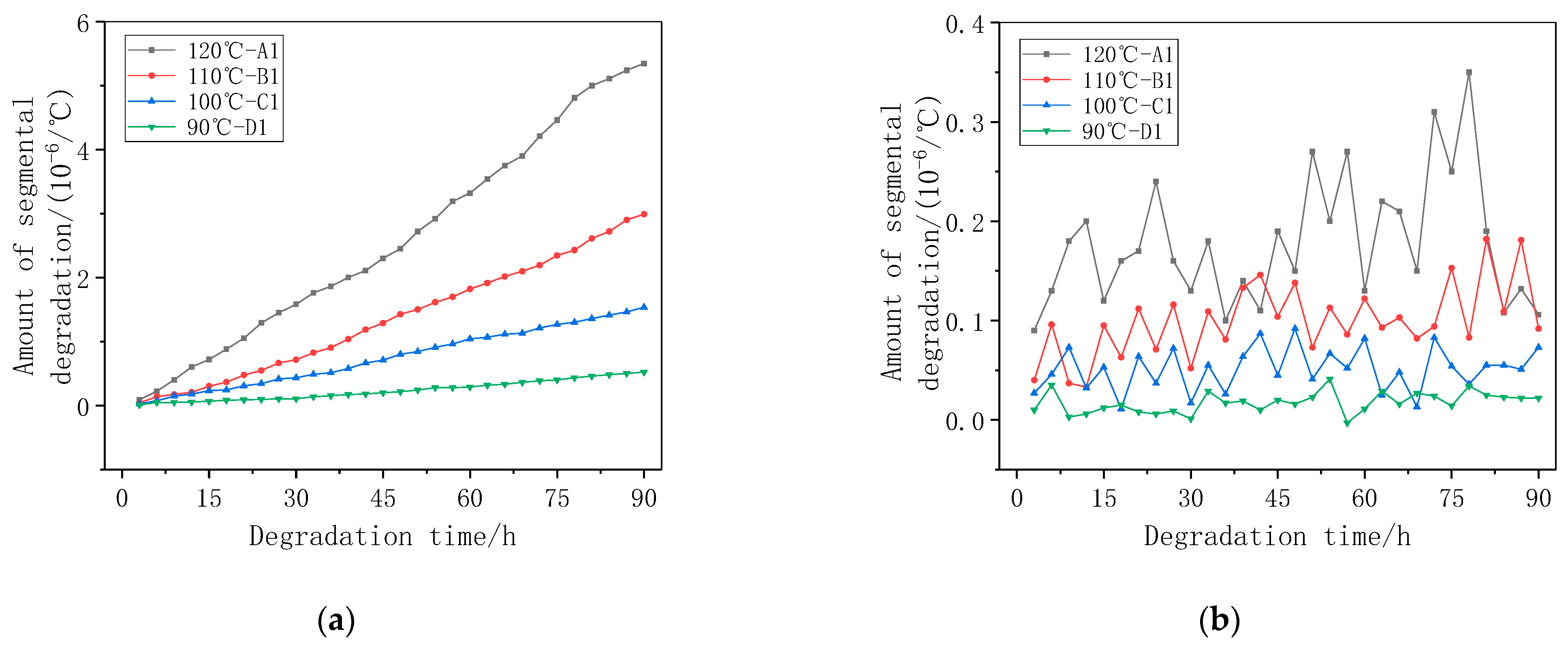
The Wiener degradation model is established according to the test data and is characterised by the degradation amount data to analyse the performance degradation process of the product. The degradation trend of the five thermal trip specimens under the same accelerated stress is basically the same [22,23], and the difference in the average degradation rate is relatively small. Take the 120°-A1, 110°-B1, 100°-C1, and 90°-D1 samples as an example to make the specific thermal deflection cumulative degradation amount of the degradation trajectory model, as shown in Figure 4a. And the degradation amount of the specific thermal deflection value of the thermal trip is segmented by time; each cycle is a time period, and the increment in the degradation of each segment is recorded as ΔX, and the change amount of the specific thermal deflection value of the bimetal of its segment is shown in Figure 4b.
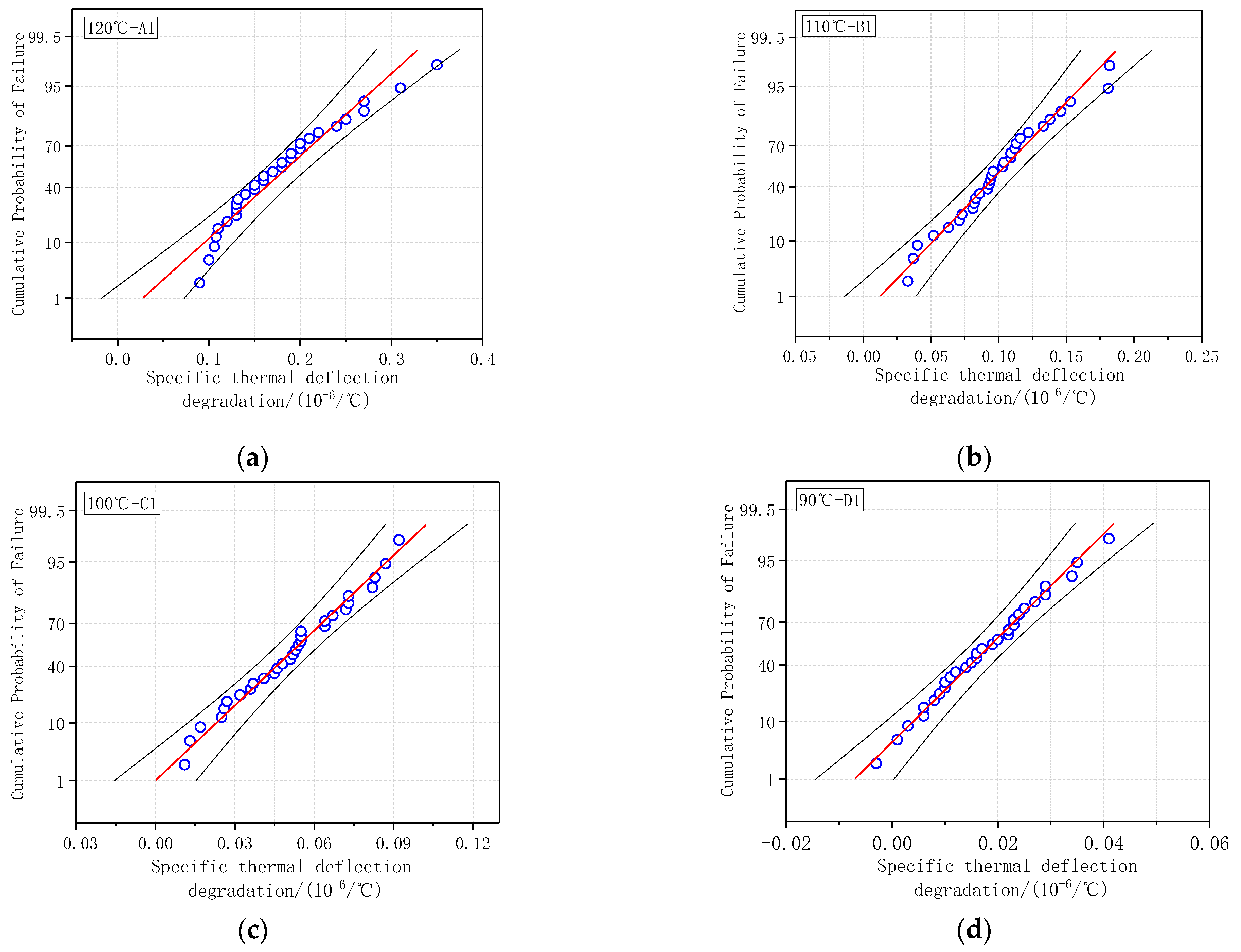
From Figure 4b, it is more intuitive to see that the specific thermal deflection degradation increment in adjacent cycles of the thermal trip is stochastic and belongs to a non-monotonic degradation process. In order to verify whether the specific thermal deflection K value of the thermal trip conforms to the normal distribution, the segmental degradation amount data of the samples A1, B1, C1, and D1 are fitted to the probability density function curve of the normal distribution with a confidence level of 95%, and the test results of the samples’ normal distribution are shown in Figure 5.
As shown in Figure 5, the vast majority of the data points are distributed on a straight line, and only a few data points fall outside the straight line. Using the knowledge of probabilistic statistics to judge, it can be assumed that the amount of segmental degradation of the low-voltage circuit breaker thermal trip over bending conforms to the normal distribution, and the Wiener degradation model can be used to compare with the bending K value modelling to achieve the reliability prediction for thermal trips of low-voltage circuit breakers. Other test samples can be verified to conform to the Wiener process using the same normal distribution test.

4.2. Residual Life Prediction of Thermal Trip Based on the Wiener Process

Taking the accelerated degradation data of the A1 specimen under the accelerated temperature stress of 120 °C as an example, the performance degradation model of the thermal trip is established, and the great likelihood estimation of the drift parameter μ can be determined as 0.1782 × 10⁻⁶/°C according to Equations (13) and (14), and the great likelihood estimation of the diffusion parameter σ can be determined as 0.0648 × 10⁻⁶/°C. The thermal trip failure threshold L = 21.811 − 13.6 = 8.211 × 10⁻⁶/°C. The failure threshold of the thermal trip is L = 21.811 − 13.6 = 8.211 × 10⁻⁶/°C. According to the performance degradation model of the thermal trip, the remaining life prediction can be made, and the remaining life probability density function and the remaining life probability density curve of the thermal trip at the initial moment can be obtained.
f ( t ) = 8.211 0.1624 t 3 e ( 8.211 0.1782 t ) 2 0.008398 t
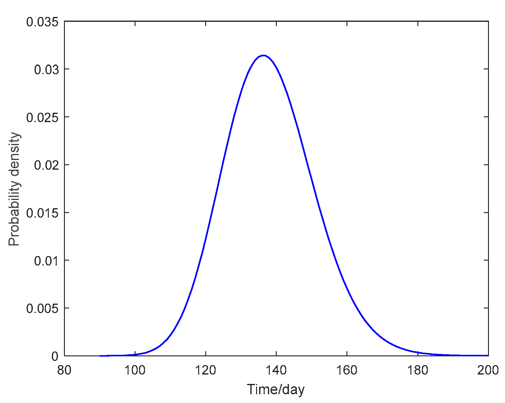
From Figure 6, it can be seen that the probability density value increases gradually with the prolongation of the degradation time, and the corresponding probability density reaches the maximum value at 137 days. The larger the probability density value, the greater the failure probability of the thermal trip. The time corresponding to the time when the probability density value reaches the maximum is taken as the residual life of the thermal trip, and it can be assumed that the residual life of sample A1 is 137 days.
Bringing μ = 0.1782 × 10⁻⁶/°C, σ = 0.0648 × 10⁻⁶/°C, and the failure threshold L = 8.211 × 10⁻⁶/°C into the above equation, the reliability function at the initial moment of the thermal trip can be expressed as follows:
R ( t ) = Φ 8.211 0.1818 t 0.0648 t exp 734.4659 Φ 8.211 0.1818 t 0.0648 t
The reliability function curve is shown in Figure 7, which shows that under the stress condition of 120 °C, the reliability of the thermal trip significantly decreases with the extension of the test cycle. According to the specification for the use of low-voltage circuit breakers, if the reliability is reduced to 0.5, it will not be able to effectively guarantee the safe operation of the power system, and the chances of the failure of the thermal trip will be greatly increased in the specified time period. According to the probability density curve of the remaining life in Figure 6 and the reliability curve in Figure 7, the reliability of 0.5 can be taken as the remaining life of the initial state of the thermal trip, and it can be assumed that the value of the remaining life of the initial moment of the A1 sample is 137 days, which is consistent with the time of the maximum failure probability in Figure 6.
The probability density curves and reliability curves of the other thermal trips samples at each accelerated stress are derived using the same calculation method to find the pseudo-failure life of each sample at different temperatures, as shown in Table 1.
The five pseudo-failure life data at each accelerated stress value in Table 1 were used as subsamples to make a normally distributed estimate of the pseudo-failure life of the thermal detent. Due to the small number of subsamples, the pseudo-failure life data at each accelerated stress value were tested for normal distribution using the S-W test. The test statistics are shown in Table 2.
The table shows that when the confidence level is 95% and the number of data points is 5, the SW test statistic is 0.762, and the test statistic of the pseudo-failure life data under each stress value in the table is greater than 0.762; therefore, it can be approximated that the pseudo-failure life of the thermal trip device obeys normal distribution. Using the great likelihood estimation method, the parameter estimates of the pseudo-failure life can be obtained from Equation (6), which is shown in Table 3.

4.3. Normal Life Expectancy Projection

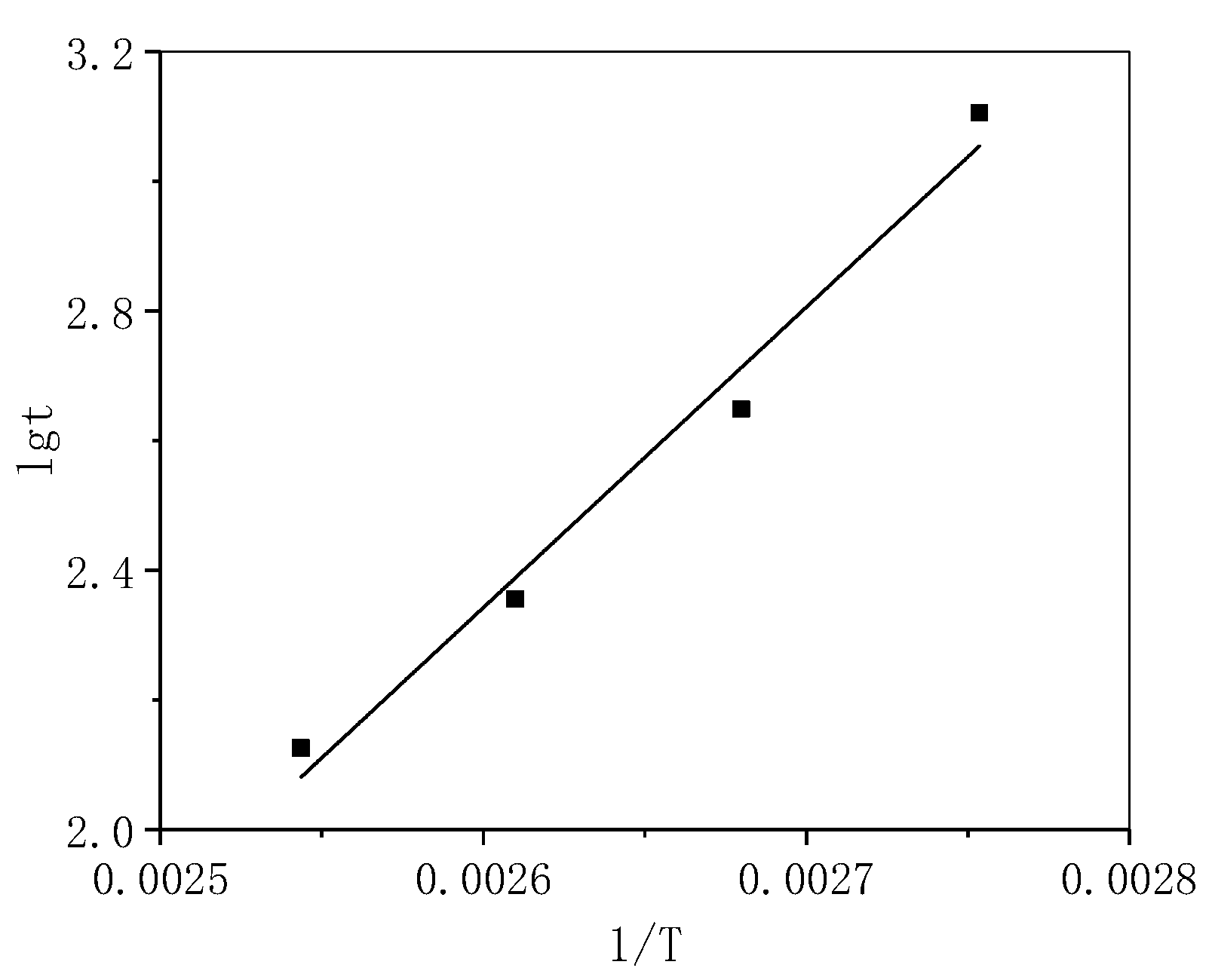
The Arrhenius model can be utilised to extrapolate the lifetime of the thermal trip under normal conditions. The pseudo-failure life values predicted in Table 3 were fitted by least squares to obtain the fitting results shown in Figure 8.
The intercept a and slope b, the correlation coefficient r, and the residual sum of squares RSS were obtained by linear regression fitting, as shown in Table 4.
The correlation coefficient is greater than 0.98, the residual sum of squares RSS is very small, approximating to 0, and the data for each residual life span are basically on a straight line, which indicates that the degree of fit is good and the linear regression effect is significant. The intercept a and slope b in Table 4 can be obtained by substituting them into Equation (5) as follows:
lg t = 9.7012 + 4632.0903 1 K
According to Equation (23), it can be extrapolated to find out that the failure time of the thermal trip of a low-voltage circuit breaker under normal operation is 6273 days. At this time, the possibility of failure of the thermal trip is greater. It can be assumed that with the growth of the use of time, the specific thermal deflection K of the thermal trip device gradually decreases. It is predicted that after about 17.2 years of use, the probability of thermal trip device’s refusal will increase greatly, and it cannot reliably complete overload protection. From the point of view of ensuring the security and stability of the power system, it should be eliminated immediately and replaced in a timely manner.

4.4. Comparison of Wiener Process and Grey-Model-Based Life Prediction

For the life prediction of highly reliable and long-life products, grey models are generally widely used for modelling. In this paper, the original measurement data of thermal detent ratio bending are accumulated to generate new data, which in turn leads to the following GM(1, 1) grey differential equation:
x ( i ) ( k + i ) + a z ( i + 1 ) ( k + i ) = b
where a is the development coefficient, which represents the development trend of the data series, and b is the grey role quantity, which represents the uncertainty of the series data.
The pseudo-failure life of the thermal trip can be predicted by Equation (24) along with the failure threshold, and the pseudo-failure life of the thermal trip obtained by Wiener’s process is listed in Table 4. The pseudo-failure life obtained using the grey model is fitted to the equation shown in Equation (25) by the least squares method, and the failure time of the thermal disconnectors of the LV circuit breakers is extrapolated to be 7079 days for normal operation, which is longer than the life predicted by the Wiener process.
lg t = 10.4125 + 4894.2798 1 T
From Table 5, it can be seen that the difference between the results of the Wiener process degradation model and the grey model on the pseudo-failure life is larger at low-temperature stresses and smaller at high-temperature stresses. Under accelerated stress at 90 °C, 100 °C, 110 °C, and 120 °C, the difference in the pseudo-failure life of the thermal disconnectors is around 156.5, 117, 52.6, and 22 days, respectively. The analysis concluded that the performance degradation rate of thermal trip at lower-temperature stress is low, and its degradation amount is also very small, which leads to the deterioration of the cumulative effect of the grey model, so that the prediction curve tends to be flat and deviates too much from the actual degradation curve, and the pseudo-failure life obtained from the prediction is too long, which is the main reason for the use of the grey model predicting that the service life under normal stress exceeds Wiener’s process by a large amount. Therefore, the lifetime prediction of the Wiener process for thermal disconnectors is more accurate than the grey model prediction.

5. Conclusions

In this paper, the thermally sensitive performance ratio bending of a thermal trip is used as the degradation characteristic quantity to establish a degradation model for the performance of a thermal trip based on the Wiener process, and the residual life prediction is carried out based on the test data of the same batch of thermal trip. The main conclusions are as follows:
(1)
The performance degradation test scheme of a thermal trip is studied, and the constant-stress-accelerated degradation test with the Arrhenius equation as the accelerated model, temperature as the accelerated stress, and specific thermal deflection K as the degradation characteristic parameter is determined. The accelerated degradation test data were analysed to reveal the performance degradation law of the thermal trip.
(2)
A thermal trip performance degradation model based on the Wiener process is established, and the degradation data under accelerated stress are segmented, with a single cycle as the time segment, and according to the central limit theorem as well as the test chart of the normal distribution of segmented degradation, checking that the segmental degradation of the specific thermal deflection obeys a normal distribution, thus conforming to the Wiener process.
(3)
In this study, we used the method of probability statistics to derive its residual life probability density function and reliability function; used the method of great likelihood estimation to obtain the estimated values of μ and σ; established the residual life prediction model of thermal trips; predicted the pseudo-failure life of thermal trips at the initial moment of accelerating stress; and externally launched the service life of thermal trips of 6273 days in the normal situation through the Arrhenius accelerating model, utilising the least-squares method of linear regression analysis. The prediction results were also compared with the pseudo-failure life obtained from the grey model prediction, and it was found that the grey model prediction was large and the Wiener process prediction was more accurate.

Author Contributions

Conceptualisation, L.W.; methodology, L.W. and X.S.; resources, Z.Z. and D.W.; writing—original draft, L.W.; writing—review and editing, L.W. and X.S. All authors have read and agreed to the published version of the manuscript.

Funding

This study was funded by the National Natural Science Foundation of China (Grant No. 51937004).

Data Availability Statement

Data are contained within the article.

Conflicts of Interest

The authors declare no conflicts of interest.

References

  1. Yao, F.; Yao, Q.; Li, X. Research on the influence of thermal bimetal on overload protection characteristics of small circuit breakers. Wenzhou, Zhejiang, Reliability Research Society of Electrotechnical Products of China Electrotechnical Society. In Proceedings of the Fifth International Conference on Reliability and Electrical Contact of Electrotechnical Products, Wenzhou, China, 16 November 2014. [Google Scholar]
  2. Zhao, J.; Yan, H.; Jiang, M. Simulation tracking method for overload relay performance degradation. Electr. Appl. Energy Effic. Manag. Technol. 2018, 39–44+54. [Google Scholar]
  3. Cheng, S.; Liu, J.; Wu, X.; Yu, T.; Xiang, C.; Yuan, D. Residual life prediction of metallized film capacitors based on feature extraction and error compensation. Chin. J. Electr. Eng. 2022, 42, 2672–2681. [Google Scholar]
  4. You, Y.; Wang, J.; Shu, L.; Ni, K.; Zhou, X. An electrical life prediction method for AC contactors based on audio features. J. Electrotechnol. 2021, 36, 1986–1998. [Google Scholar]
  5. Chen, L.; Chen, J.; Wang, H.; Wei, H.; Pan, H. Remaining battery life prediction based on wavelet packet energy entropy. J. Electrotechnol. 2020, 35, 1827–1835. [Google Scholar]
  6. Liu, G.; Wang, Z.; Li, X.; Zhao, X.; Miao, J. Reliability assessment of electronic residual current operated circuit breakers based on improved Bootstrap-Bayes. J. Electrotechnol. 2022, 37, 4250–4258. [Google Scholar]
  7. Feng, H.; Wang, Y. Reliability analysis of performance degradation products based on support vector regression and Bayesian theory. J. Nanjing Univ. (Nat. Sci.) 2019, 55, 161–169. [Google Scholar]
  8. Zhang, Z.; Xu, X.; Yu, J. Study on life prediction of contactor in traction system of rolling stock based on accelerated life test. Railw. Roll. Stock. 2023, 43, 37–44. [Google Scholar]
  9. Li, K.; Gao, Z.; Wu, Y.; Zheng, S.; Li, J. Residual life prediction of AC contactors based on statistical regression and nonlinear Wiener process. J. Electrotechnol. 2019, 34, 4058–4070. [Google Scholar]
  10. Chen, L.; Wang, H.M.; Chen, J.; An, J.; Ji, B.; Lyu, Z.; Cao, W.; Pan, H. A novel remaining useful life prediction framework for lithium-ion battery using grey model and particle filtering. Int. J. Energy Res. 2020, 44, 7435–7449. [Google Scholar] [CrossRef]
  11. Li, K.; Li, X.; Zheng, S.; He, J.; Wu, Y. Residual electric life prediction of AC contactors based on BP neural network. J. Electrotechnol. 2017, 32, 120–127. [Google Scholar]
  12. Zhang, L.; Xita, A.; Tian, X.; Li, W. Multi-objective optimization design of accelerated degradation test based on Gamma process. J. Jilin Univ. (Eng. Ed.) 2022, 52, 361–367. [Google Scholar]
  13. BS EN 60947-2:2016; Low-Voltage Switchgear and Controlgear—Part 2: Circuit-breakers. International Electrotechnical Commission: Geneva, Switzerland, 2016.
  14. GB/T 14048.2-2020; Low-Voltage Switchgear and Controlgear—Part 2: Circuit-breakers. GB: Beijing, China, 2020.
  15. GB/T 2689.1-1981; General Rules for Constant Stress Life Test and Accelerated Life Test Method. National Technical Committee for Standardization of Low-Voltage Electrical Appliances: Shanghai, China, 1981.
  16. Liu, J.; Chen, A.; Yan, Y.; Zhang, M.; Qi, H. Reliability assessment method of electromagnetic contactors for high-speed trains. J. Electrotechnol. 2018, 33, 461–471. [Google Scholar]
  17. Li, J.; Huang, J.; Qiu, M.; Wang, Z.; Pang, X.; Dong, Y. Residual life prediction of rolling bearings based on generalized Wiener process. Comput. Integr. Manuf. Syst. 2022, 28, 1–17. [Google Scholar]
  18. Zhang, X.; Gockenbach, E.; Liu, Z.; Chen, H.; Yang, L. Reliability estimation of high voltage SF6 circuit breakers by statistical analysis on the basis of the field data. Electr. Power Syst. Res. 2013, 103, 105–113. [Google Scholar] [CrossRef]
  19. Lee ML, T.; Whitmore, G.A. Threshold regression for survival analysis: Modeling event times by a stochastic process reaching a boundary. Stat. Sci. 2006, 21, 501–513. [Google Scholar]
  20. Folks, J.L.; Chhikara, R.S. The Inverse Gaussian Distribution and Its Statistical Application—A Review. J. R. Stat. Soc. 1978, 40, 263–289. [Google Scholar] [CrossRef]
  21. Sawa, K.; Yoshida, K.; Watanabe, M.; Suzuki, K. Arc characteristics and electrode mass change of Ag-Ni contacts for electromagnetic contactors. In Proceedings of the 56th IEEE Holm Conference on Electrical Contacts, Charleston, SC, USA, 4–7 October 2010; pp. 1–6. [Google Scholar]
  22. Tang, S.; Guo, X.; Yu, C.; Zhou, Z.; Zhou, Z.; Zhang, B. Real time remaining useful life prediction based on nonlinear Wiener based degradation processes with measurement errors. J. Cent. South Univ. 2014, 12, 4509–4517. [Google Scholar] [CrossRef]
  23. Zhu, L.; Zuo, H.; Cai, J. Reliability prediction of civil aviation engine performance based on Wiener process. J. Aerosp. Dyn. 2013, 28, 1006–1012. [Google Scholar]
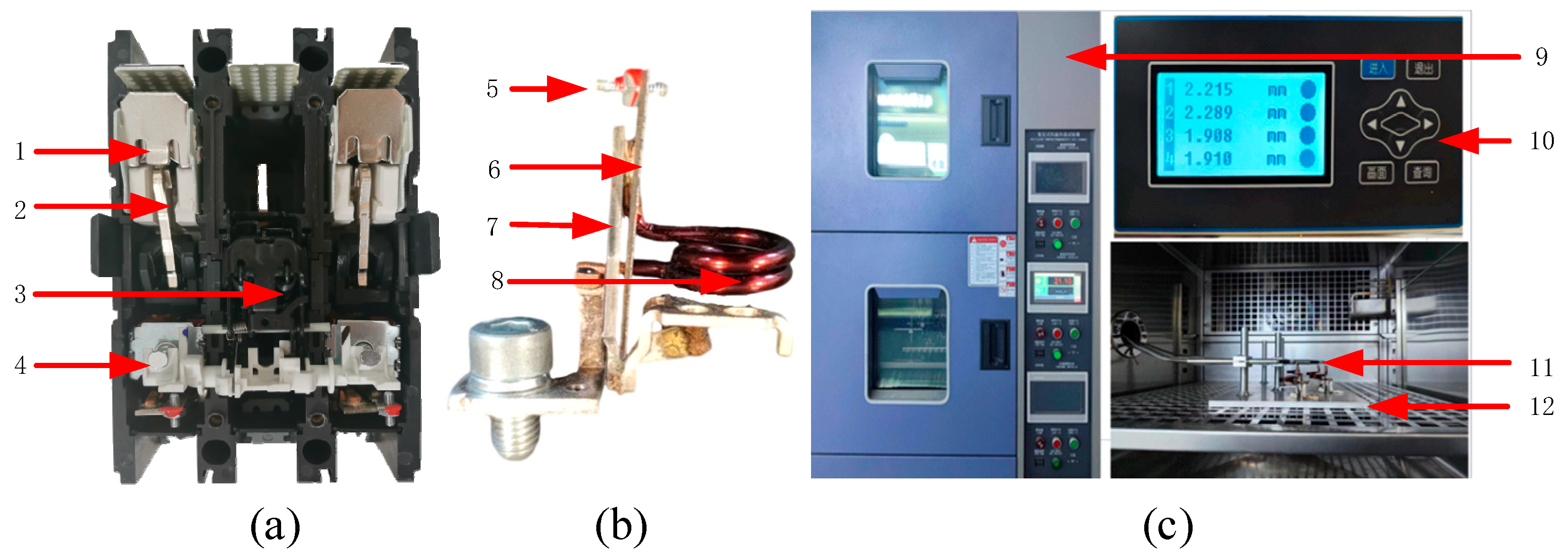
Figure 1. Low-voltage circuit breakers and measuring devices. (a) Low-voltage circuit breaker, (b) thermal trip, (c) measuring devices. 1—interrupting chamber, 2—active and static contacts, 3—operating mechanism, 4—thermal magnetic trip, 5—adjusting screw, 6—hot bimetal, 7—heating element, 8—electromagnetic coil, 9—constant-temperature and constant-humidity box, 10—deflection display, 11—high-precision displacement sensor, 12—base.
Energies 17 01189 g001
Figure 2. Specific thermal deflection degradation at the same stresses.
Energies 17 01189 g002
Figure 3. Schematic diagram of residual life prediction.
Energies 17 01189 g003
Figure 4. (a) Cumulative degradation over bending. (b) Specific thermal deflection Segment Degradation Volume.
Energies 17 01189 g004
Figure 5. (a) A1 normal distribution test probability plot; (b) B1 normal distribution test probability plot; (c) C1 normal distribution test probability plot; (d) D1 normal distribution test probability plot.
Energies 17 01189 g005
Figure 6. Probability density curve of remaining life of thermal trip at 120 °C.
Energies 17 01189 g006
Figure 7. Reliability curves of samples under stress at 120 °C.
Energies 17 01189 g007
Figure 8. Least squares fitting results.
Energies 17 01189 g008
Table 1. Pseudo-failure life of thermal trip.
Temperature/°CSerial NumberPseudo-Failure Life/DayTemperature/°CSerial NumberPseudo-Failure Life/Day
120A1137100C1441
A2144C2411
A3150C3393
A4141C4426
A5129C5456
110B123790D11350
B2249D21416
B3219D31410
B4213D41392
B5216D51425
Table 2. Test statistics.
Temperature/°CStatistic
900.8757
1000.9786
1100.8714
1200.9920
Table 3. Estimated value of thermal trip parameters.
Temperature/°Cμ/Dayσ/Day
901398.629.73
100425.424.68
110226.815.53
120139.87.85
Table 4. Linear regression fitted parameter values.
ParametersabrRSS
Numerical value−9.70124632.09030.982180.0098
Table 5. Pseudo-failure life of Wiener and grey model.
Temperature
/°C
Wiener Pseudo-Failure Life/DayGrey Pseudo-Failure Life/DayDifference/Day
901398.61555.1156.5
100425.4542.4117
110226.8279.452.6
120139.8161.822
Disclaimer/Publisher’s Note: The statements, opinions and data contained in all publications are solely those of the individual author(s) and contributor(s) and not of MDPI and/or the editor(s). MDPI and/or the editor(s) disclaim responsibility for any injury to people or property resulting from any ideas, methods, instructions or products referred to in the content.