A Novel Approach to Dynamic Line Rating Calculation

Abstract

In order to adjust the electric power network to today’s trends—such as the charging of electric vehicles, design of the Internal Electricity Market (IEM), headway of renewable energy sources, etc.—the demand for flexible network solutions is increasingly significant. Dynamic line rating (DLR) technology offers a flexible solution for the uprating of overhead lines. Moreover, the DLR methodology can be used in a wider system approach in order to establish a line management system, including functions such as ice prevention subsystems or the real-time tracking of clearances. Therefore, the extension possibilities and operational features of DLR-based systems have been extensively researched in the last few years, which is also confirmed by the high number of pilot projects funded for research and development on the topic of DLR. The key question during the implementation of a DLR system is the obtainable operational safety of such a system. This mainly depends on the installation places of the field equipment and the accuracy of the line rating calculation models. The aim of this article is the comparison of the so far available international line rating calculation models and also to propose another way for the determination of the real-time line rating. Moreover, laboratory measurements and case studies are presented for the confirmation of the proposed model’s reliability.

1. Introduction

During the operation of their networks, electric power system operators have to face the challenges caused by the altering practices and trends, both on the generation and consumer side. The spreading of electric vehicles, especially by considering fast-charging stations, requires the reinforcement of the critical parts of the grid or the enhanced utilization of the existing infrastructure [1]. In the European Union, the renewable energy share target that it desires to reach until 2030 is 32% [2], which affects the grid loads in an intermittent way, for that the capacity of the lines have to be adjusted [3]. Besides these challenges, the electrification of more and more household equipment and the increasing industrial electricity consumption also contribute to the growing energy demand [4], which means higher peak loads on the grid, too [5]. Furthermore, the liberalization of the electricity market, the market environment and consumer habits are also changing, on which is based the European Union’s Second Energy Package targeted at the formation of the Internal Electricity Market (IEM) in its medium- and long-term strategy [6]. The implementation of the IEM requires the strengthening of cross-border connections in order to reach higher transmission capacities. Moreover, the physical energy flows coming from the loop flows and the export–import market actions between the European countries also impose a significant burden on the cross-border transmission lines [7].

All the described challenges during the operation of the electric power grid lack the implementation of flexible network solutions in order to keep sustainable the existing infrastructure in the long term. Moreover, the consumers’ needs have to be satisfied using an aging network [8], thus the continuous monitoring of the system elements is essential during the implementation of uprating technologies. Dynamic line rating (DLR) technology offers a possible solution for handling these challenges in the case of overhead lines. Conventionally, the maximum allowed transmission capacity of the power lines is determined with the so-called static line rating (SLR) calculation method. By calculating the SLR of a power line, the worst-case environmental parameters are considered in order not to exceed the maximum allowed conductor temperature by applying this line load during any weather condition. However, SLR is a safe capacity allocation method from a thermal point of view; on the other hand, it is wasteful in the utilization of the infrastructure [9]. Contrarily, the essence of the dynamic line rating method is to measure the environmental parameters along the line corridor, from which the actual line rating can be calculated by modeling the thermal heat balance of the conductors. By using the DLR capacity allocation method, the obtainable surplus capacity is 25–40% on average compared to the SLR capacity constraints [10,11].

As the DLR system requires different input parameters for the calculation, such as the measurement of weather parameters, conductor temperature, line load or weather forecast for line rating forecast, the DLR system can be extended by different subsystems on the basis of the same input parameter list. One extension possibility is the real-time monitoring of the sag-clearance values in the critical spans, where conductor temperature measuring sensors are applied. In this way, the standard regulated ground clearance levels and clearances from objects under the line can be maintained at every conductor temperature that occurs during the operation of overhead lines with the DLR capacity allocation method. Another supplementary function that can be achieved with the DLR-based line management system is the ice forecasting subsystem. In this case, the weather forecast used for the line rating prediction is also used to determine if the environmental conditions are favorable for ice formation on the conductors. If so, other properties of the expected ice layer—like the ice type, mass of the ice sleeve and its radius—are also determined. Moreover, the anti-icing current can be also calculated by the DLR algorithm. In this way, system operators have comprehensive information about the risk of icing with the required prevention interventions [12]. Altogether, the implementation of a DLR or a DLR-based line management system has many advantages not only in the field of uprating power lines but also in the safe and reliable operation. For the safe operation, the forecasting and prevention of icing events, or the avoidance of thermal overloads of the conductors, can be examples. Regarding the reliable operation, the more precise generation schedule planning based on the ampacity forecast means a practical pattern [13,14].

Besides the several advantages of DLR system realization, there are many open research areas in this field. As different international models are available for line rating calculation purposes, one of these research fields is the evaluation and fine-tuning of these models. The current transmission capacity models show high deviation compared to each other, especially in the case of low wind speed, where the calculated ampacity is the most sensitive to the wind speed and direction [15,16]. Moreover, the weather-based calculation models provide volatile ampacity values [17], which are hard to consider at the dispatchers’ side as a capacity constraint. This article aims to investigate the international models’ accuracy in a direct way with laboratory measurements as so far only indirect validation results are available in the international literature [18,19,20]. Then, the article proposes a new way of thinking in the calculation of transmission capacity with DLR methodology. In order to evaluate the performance of the proposed algorithm and compare with the so far existing methods, laboratory measurements on different conductor types are also carried out. The testing of the developed algorithm under real field conditions and the investigation of its practical application are also the aim of our research.

2. Dynamic Line Rating Calculation Methods

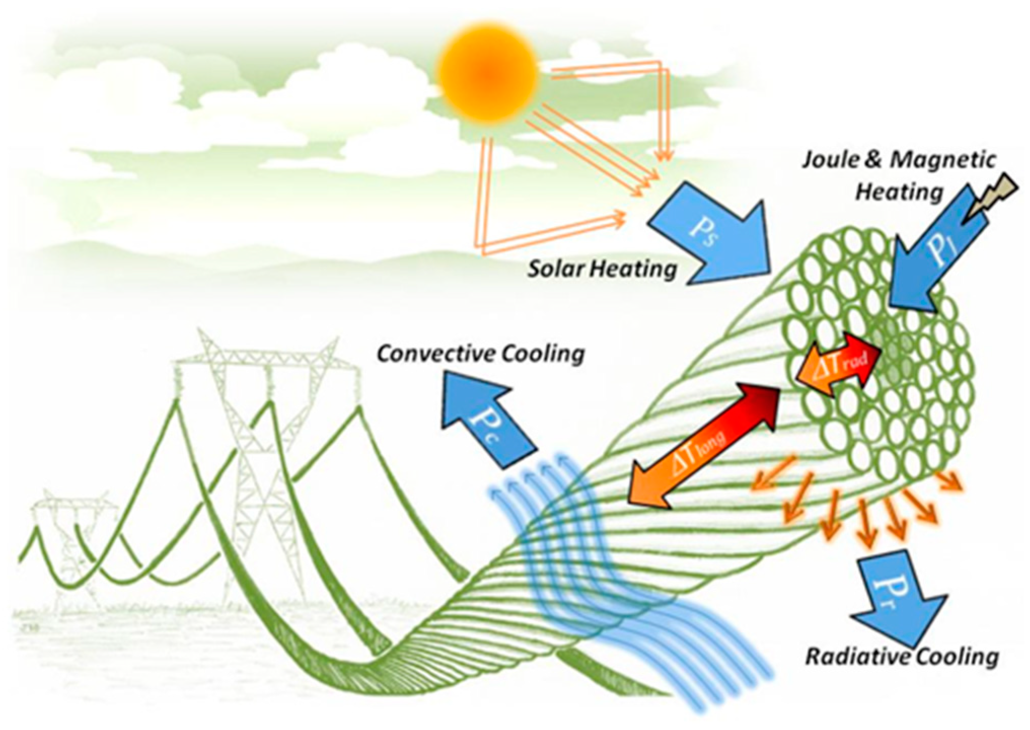
The basis of the internationally available dynamic line rating calculation methods is the modeling of the thermal state of the phase conductors. For that purpose, the weather conditions along the line should be measured. By measuring the environmental conditions, the heat balance of the conductors can be written, where the heating and cooling effects of the environment keep the heat balance with the Joule-heating caused by the current flowing through the conductor. The covered environmental parameters are the convective cooling caused by the wind, the radiative cooling based on the temperature difference of the conductor and the surrounding air and the heating of the solar radiation. The schematic of the environmental factors affecting the thermal sate of the conductors is shown in Figure 1.

With the rearrangement of the thermal equilibrium equation of the conductors, the maximum current depending on the weather conditions can be calculated. All three internationally available models are based on this calculation method, namely the Cigre [21], IEEE [22] and IEC [23] ones.

The sensor manufacturers and the utilities are preferring the Cigre and IEEE models to a similar extent during the implementation of DLR systems, while the use of the IEC model is not common in practice. There are several papers in the international literature for the comparison of the two most common models, which point out the uncertainty of the Cigre and IEEE models compared to each other. Ref. [24] compares the two models in an indirect way through the conductor temperature determination, of which the main finding is that a higher deviation occurs in cases of low wind speeds. Ref. [25] shows that the deviation of the calculated conductor temperature with the international models can reach 20 °C in 10% of the time, on which basis the uncertainty of the calculated ampacity was validated. Ref. [26] presents simulations about the ampacity calculated for a wide range of wind speeds, directions and ambient temperatures, both with the Cigre and IEEE models, on which basis a 20% difference was observed in some conditions. Ref. [27] identifies 5–15% variation between the Cigre and IEEE dynamic line rating models. Ref. [28] uses indirect validation by comparing the conductor temperature calculated with the international models with the field measurements and identifies a more than 5 °C peak deviation. Ref. [29] compares the two models via simulation, where more than a 25% deviation can be observed during high wind speed conditions. Altogether, it can be seen from the international literature that there are only comparisons based on modeling and indirect validation that are available for the determination of the current models’ accuracy, which implies the need for direct validation of the so far existing calculation methodologies. Moreover, as high as 25% deviation is identified by some research, which endorses the development of new models.

As the international models have some neglections in the heat balance equation—such as they do not take into account the cooling effect of precipitation or the heating effect of corona discharges—the extension of the so far available calculation methods is one way of fine-tuning the DLR algorithms [30]. Contrarily to the international models, the most accurate model can be achieved by the direct measurement of the conductor temperature, as in this case all the environmental and electrical factors that affect the conductor’s thermal state are taken into consideration through field measurements, as well the thermal inertia of the conductors, which appears in the less fluctuating—therefore, more practical—ampacity results. Furthermore, by measuring the actual conductor temperature, this information can be further used. One useful application of conductor temperature measurement is to avoid conductor annealing by maintaining the temperature under the threshold limit of annealing. Furthermore, it is useful to calculate the actual sag of the conductors, which is essential for the ground clearance modeling that should be kept during all operation conditions, which is especially important in case of the higher thermal utilization of the conductors during the operation of a DLR system. These considerations together were the motivation for the line rating calculation model development based on conductor temperature measurement.

2.1. Analogies of Existing Line Rating Calculation Models

The three cited DLR calculation models are using the same heat balance equation described by (1).

$$P_J+P_s=P_r+P_c$$

(1)

where P_J is the Joule-heating effect [W/m], P_s is the solar-heating effect [W/m], P_r is the radiative-cooling effect [W/m] and P_c is the convective-cooling effect [W/m]. As it can be seen from (1), all the environmental heating and cooling effects and also the Joule-heating are expressed in W/m dimension in the heat balance equation.

By rearranging (1), the ampere capacity (ampacity) of the given conductor can be obtained in the ampere dimension with (2).

$$I=\sqrt{\frac{P_r+P_c-P_s}{R_{AC}}}$$

(2)

where R_AC is the AC resistance of the conductor at its maximal continuous operational temperature [Ω/m].

2.1.1. Joule-Heating Calculation

The Joule- or Ohmic-heating is caused by the non-zero resistance of the conductor with which it is directly proportional, while it is squarely proportional to the current flowing through the conductor, as it is described by (3).

$$P_J=I^2·R_{AC}$$

(3)

where I is the conductor load [A] and R_AC is the AC resistance of the conductor at its maximal continuous operational temperature.

The AC resistance of the conductor is usually not available in the conductor’s technical data sheet, especially in the case of higher conductor temperatures. In order to obtain this value, both the Cigre [21] and IEEE [22] methods explain the skin effect on the AC resistance calculation. Moreover, for the determination of the AC resistance at the maximal continuous operational temperature, both models offer a linear interpolation method, which requires the conductor AC resistance at two different temperatures to calculate the maximum temperature value.

2.1.2. Calculation of Solar Heat Gain

As in the case of Joule-heating determination, the effect of solar heat gain is also determined with the same equation in the three international models. The heat gain caused by the solar radiation is proportional to the intensity of the global radiation, the diameter of the conductor and the absorptivity of the conductor’s surface, as it is written by (4).

$$P_s=I_s·D·K_a$$

(4)

where I_s is the intensity of the global radiation [W/m²], D is the conductor’s diameter [m] and K_a is the absorption coefficient [-]. The non-dimensional absorptivity factor is depending on the conductor’s condition, mostly on its age and the environment where it is used. The Cigre technical brochure [21] offers some instruction for the estimation of the conductor’s absorptivity.

2.1.3. Determination of Radiative Cooling

The Stefan–Boltzmann law is used by all three international models in order to determine the radiative-cooling effect on the conductor. The Stefan–Boltzmann law describes the emitted heat power of a black body in terms of its absolute temperature. Accordingly, the emitted heat power is proportional of the emissivity factor and the black body’s absolute temperature. The non-dimensional emissivity factor should be used for the so-called gray bodies, whose heat emission is less than the black bodies. The Stefan–Boltzmann law for phase conductors is expressed by (5).

$$P_r=\pi ·{\sigma }_B·D·K_e·\left[{\left(T_c+273\right)}^4-{\left(T_a+273\right)}^4\right]$$

(5)

where σ_B is the Stefan–Boltzmann constant [W/m²·K⁴], D is the conductor’s diameter [m], K_e is the emissivity factor of the conductor’s surface [-], T_c is the conductor’s temperature [°C] and T_a is the ambient temperature [°C]. As in the case of the absorption coefficient, the Cigre technical brochure [21] also offers recommendations for the estimation of the emissivity factor depending on the age of the conductor.

2.2. Divergencies of Existing Line Rating Calculation Models

However, the Joule-heating, while the solar heat gain and the radiative-cooling are determined in the same way with the three different international DLR models, the convective cooling caused by the wind is modeled in different ways. By also considering that the wind—both the wind speed and direction—has the largest impact on the line rating, it can be concluded that the different modeling of the convective-cooling can cause large deviations between the line ratings calculated by the different models [15,31]. The deviation between the models also depends on the conductor parameters, from which the maximal continuous operating temperature has the largest impact.

Cigre TB601 uses a fluid dynamics model for the convective-cooling calculation caused by the wind. For this purpose, the so-called Nusselt number is determined, which characterizes the ratio of convective to conductive heat transfer at a boundary surface. The Nusselt number is calculated through the determination of the Reynolds number, which identifies flow patterns, namely that the fluid flow tends to be dominated by turbulent or laminar flow. For that purpose, the Cigre model uses two coefficients depending on the roughness of the conductor’s surface and the type of the conductor. These coefficients can be obtained from a table described in the technical brochure. In order to take into account the effect of the wind direction, the equations proposed by Morgan [32] are used to compensate the convective-cooling calculated for perpendicular air flows depending on the conductor type and the attack angle. This compensation is particularly important because the air flows parallel to the conductor only mean a 42% cooling effect compared to the perpendicular flows. Moreover, the Cigre model calculates the natural convention besides the forced convection discussed so far. Natural convection acts at low or zero wind speeds, when the heat transport mechanism is not led by externalities but by the buoyancy effect of the temperature gradients. During the calculation of the convective-cooling, both natural and forced convection are determined, from which the dominant should be taken into account during the determination of the line rating [21].

IEEE Std 738 [22] uses the convection calculation method suggested by [33]. IEEE also determines both the natural or free convection during still air conditions and the forced convection due to moving air around the conductors. The proposed equations are based on large-scale wind tunnel measurements. At low wind speeds, the larger value from the free convection and forced convection values should be considered, while in the case of higher wind speeds, the calculation result of forced convection will be the dominant. Regarding the effect of the wind attack angle, the IEEE formula determines a so-called K_angle factor in a closed formula, which reduces the wind effect put up by perpendicular wind [22].

The simplest formula for the calculation of the convective heat loss is proposed by the IEC method. In this calculation method, only the forced convection is determined with the use of the Nusselt number; however, this model recommends a more elementary way to determine it than in the case of the Cigre method. On the other hand, the wind direction effect is also neglected, and this standard does not require the use of the effective wind speed for the calculation. Accordingly, the convective-cooling effect calculation is least accurate according to the IEC calculation method from the three international models [23].

2.3. Comparison of Line Rating Determined with the Different Existing Models

The previous subsection showed that the three international line rating calculation methods have the same formulas for the determination of the Joule-heating, solar heat gain and radiative-cooling effects. On the other hand, the convective-cooling caused by the wind is determined in three different ways, from which in advance the IEC method seems the most inaccurate. In order the investigate what is the deviation of the three models regarding each other, two case studies are presented here. During the first case study, the convective-cooling values determined by the three formulas—as it is the only dissimilar parameter—are compared to each other, while in the second case study, the line rating values are compared. In order to obtain a more comprehensive picture regarding the practical application of these models, the case studies are carried out for two different types of conductors, which are most commonly used in the European transmission system. In the case of the ambient conditions during the simulations, the most prevailing wind properties (wind speed ≤ 5 m/s and attack angle of between 0–90°) are considered. The main parameters of the two ACSR conductors are summarized in

Table 1. Technical parameters of the conductors used in the case studies [34,35].

Parameter		Value		Dimension
Symbol	Denomination	Hawk	500/65 ACSR
q (Al/St)	Cross-section area	240/40	500/65	mm2
No.strands	Structure of strands	7 × St + 26 × Al	7 × St + 54 × Al	-
Dcond	Overall diameter	21.79	31.06	mm
dstrand	Strand diameter (Al)	2.68	3.45	mm
RAC	AC resistance	120.09 @ 25 °C 143.71 @ 75 °C	58.50 @ 20 °C 67.32 @ 60 °C	mΩ/km mΩ/km

.

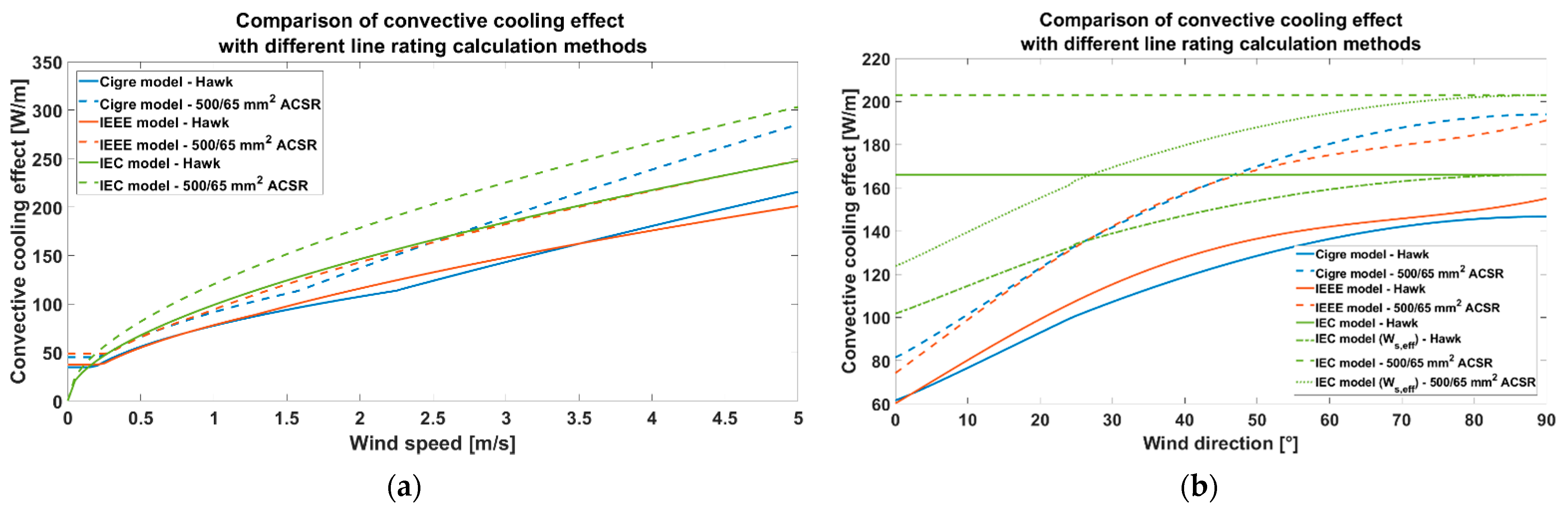
During the first simulation, the convective-cooling effect values calculated with the three international models as a function of the wind speed and wind direction are determined. For this purpose, the other environmental parameters are fixed at a constant value, namely the ambient temperature at 20 °C and the wind direction at 45° while investigating the wind speed dependency, and the wind speed at 2.5 m/s while examining the wind direction dependency. The wind speed is fixed at 2.5 m/s because the Cigre and IEEE models have the slightest deviation at this wind speed. Accordingly, the wind direction effect can be investigated more accurately at this fixed point. The maximal continuous operational temperature of the conductors is chosen as 80 °C, as this limit value is widely applied in the European practice to determine the SLR.

Figure 2a shows that the IEEE and Cigre models have less deviation compared to each other, especially in the case of the conductor with lower cross-section area. Moreover, the graph visualizes that the IEC model does not take into consideration the natural convection, because the convective-cooling calculated with the IEC model decreases to 0 W/m, while the other two models have a constant natural-cooling effect under the wind speed of 0.2 m/s. Figure 2b illustrates how the wind direction effects the convective-cooling in the case of the different models. The same tendencies can be observed regarding the models’ deviation compared to each other as in the case of wind speed dependency. As the IEC model does not take into account the wind direction effect, the convective-cooling effect is also determined as a function of effective wind speed in this case, which is the equivalent perpendicular wind speed that takes into account the wind speed and its attack angle in the case of a non-perpendicular wind. However, it amends the trend of the outputs, meaning the relative discrepancy is still much higher than between the other two models. These simulations confirm the prior expectations that the IEC model has higher deviation from the IEEE and Cigre models. By also considering that the IEEE and Cigre models are the two most commonly used ones, the IEC model is not examined in the following parts of the paper.

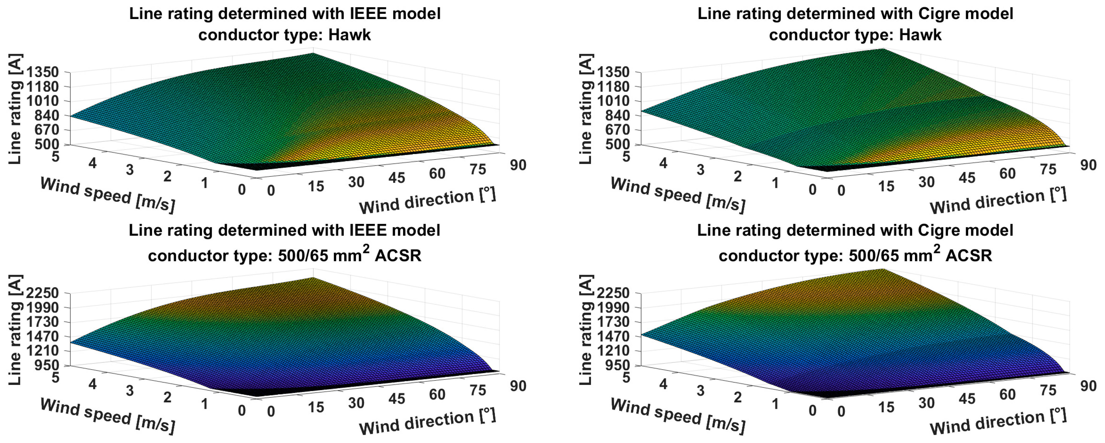
In order to investigate how the different modeling of the convective-cooling affecting the line rating overall, a case study is also carried out. Figure 3 shows how the line rating is influenced by the wind speed and direction modeled by the IEEE and Cigre calculation methods for the 500/65 mm² ACSR and Hawk conductors.

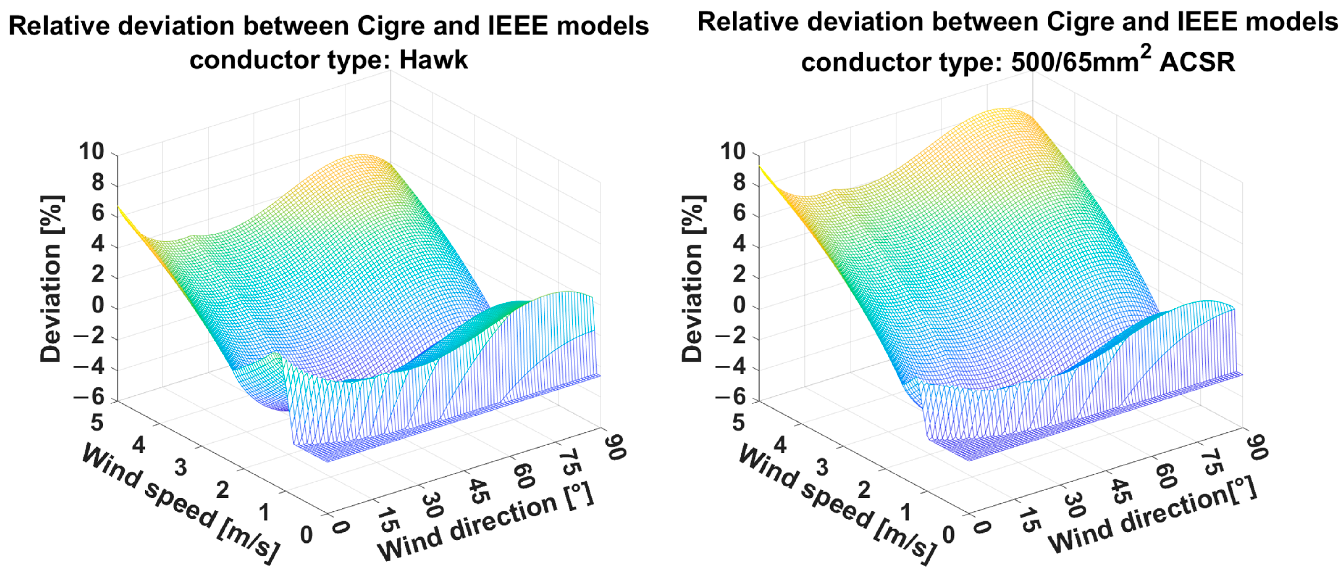
Figure 3 shows that the line rating calculated with the Cigre and IEEE models can differ by some hundred amps during casual weather conditions when the wind speed does not exceed 5 m/s. Figure 4 presents the relative deviation between the models for an even more insightful comparison.

Figure 4 shows that the relative deviation is higher in the case of the conductor with larger cross-section area. In the case of the Hawk-type conductor, the maximum difference is 6.76%, while it is 9.39% for the 500/65 mm² ACSR conductor. These deviations can be considered as the line rating uncertainty in the case of regular weather conditions, if the other input parameters (both the measurement of the weather parameters and the technical properties of the conductor) are known without any uncertainty or measurement deviation. As this is not possible in practice, the determined line rating’s uncertainty can exceed 10%. In order to investigate the exact uncertainty, laboratory measurements are carried out, and for the reduction of this uncertainty, a new line rating calculation methodology is proposed.

3. Line Rating Determination without Weather Parameters

As the previous section showed, the uncertainty of the line rating calculation is coming from the different modeling of the wind effect and the uncertainty of the input parameters, which can reach nearly 10% compared to each other. As the existing ampacity calculation methods determine the line rating through the heat balance equation, these can be considered as indirect methods. The weather stations are normally installed at lower altitudes than the position of the phase conductors because of the accessibility of the energized parts of the line, or even weather stations in open areas provide weather data for calculation, which also increases the uncertainty of the calculated line rating [36]. Moreover, no direct validation is available in the international literature (just only conductor temperature tracking-based information). All in all, these sources of inaccuracy led to the re-thinking of the line rating calculation methods.

3.1. Proposed Model

The main goal during the concept pattern was to increase the operational safety level of the line rating calculation by using direct field measurement. From the possible measured parameters, the conductor temperature was chosen for several reasons. The first reason is that the sag and hence the ground clearance level is directly correlated with the conductor temperature. Therefore, if the conductor temperature is measured, system operators have real information regarding the ground clearance level, which is the most critical legally regulated safety pattern. The second reason is that the permanent degradation and therefore the reduction of the lifetime of the conductors is directly linked to their temperature. Thermal overloads exceeding 93 °C in the case of conventional ACSR conductors are causing a loss of strength due to the annealing of the Al conductor strands [37,38,39,40]. By monitoring the conductor temperature, the annealing process also can be eliminated from the operational risks. Accordingly, the lifetime of the conductors can be extended even in the case of operation at elevated temperatures. Furthermore, all the existing line rating calculating models have some neglection in the heat balance equation, such as the corona heat effect, magnetic heating or the evaporative-cooling [41]. Altogether, using the measured conductor temperature in order to calculate ampacity has several advantages contrary to the weather-based indirect models.

The conductor can be modeled as a single heat storage system from the thermal behavior point of view, where transient thermal equation is described by (6).

$$\frac{dQ}{dt}=m·C_p·\frac{dT}{dt}$$

(6)

where Q is the heat energy per unit length of the conductor [W/m³], m is the specific mass of the conductor [kg/m], C_p is the heat capacity of the conductor [J/kg·K], dT is the temperature change of the conductor [°C] and dt is the inspected time interval [s].

Similar to the existing methods, it is assumed that the dQ/dt change in the thermal energy of the conductor is only generated by the load change, or in other words, the effect of weather condition changes on the thermal energy of the conductor is only considered at every calculation step, but not between the calculation steps. Accordingly, the thermal energy balance equation of the conductor can be expressed with (7).

$$\frac{dQ}{dt}=I_{surplus}^2·R_{AC}\left(T\right)$$

(7)

where I_surplus is the surplus current that is permissible beside the actual load of the conductor not to exceed its maximal continuous operational temperature [A] and R_AC(T) is the temperature-dependent AC resistance of the conductor [Ω/m].

By rearranging (6) and (7), the dynamic line rating of a single conductor can be expressed with (8).

$$I=I_{load}+\sqrt{\frac{m·C_p·dT}{R_{AC}\left(T\right)·dt}}$$

(8)

where I_load is the actual load of the conductor [A]. In the case of bundled conductors, the result of (8) should be multiplied by the number of bundles in order to obtain the line rating of a phase.

3.2. Model Validation with Laboratory Investigations

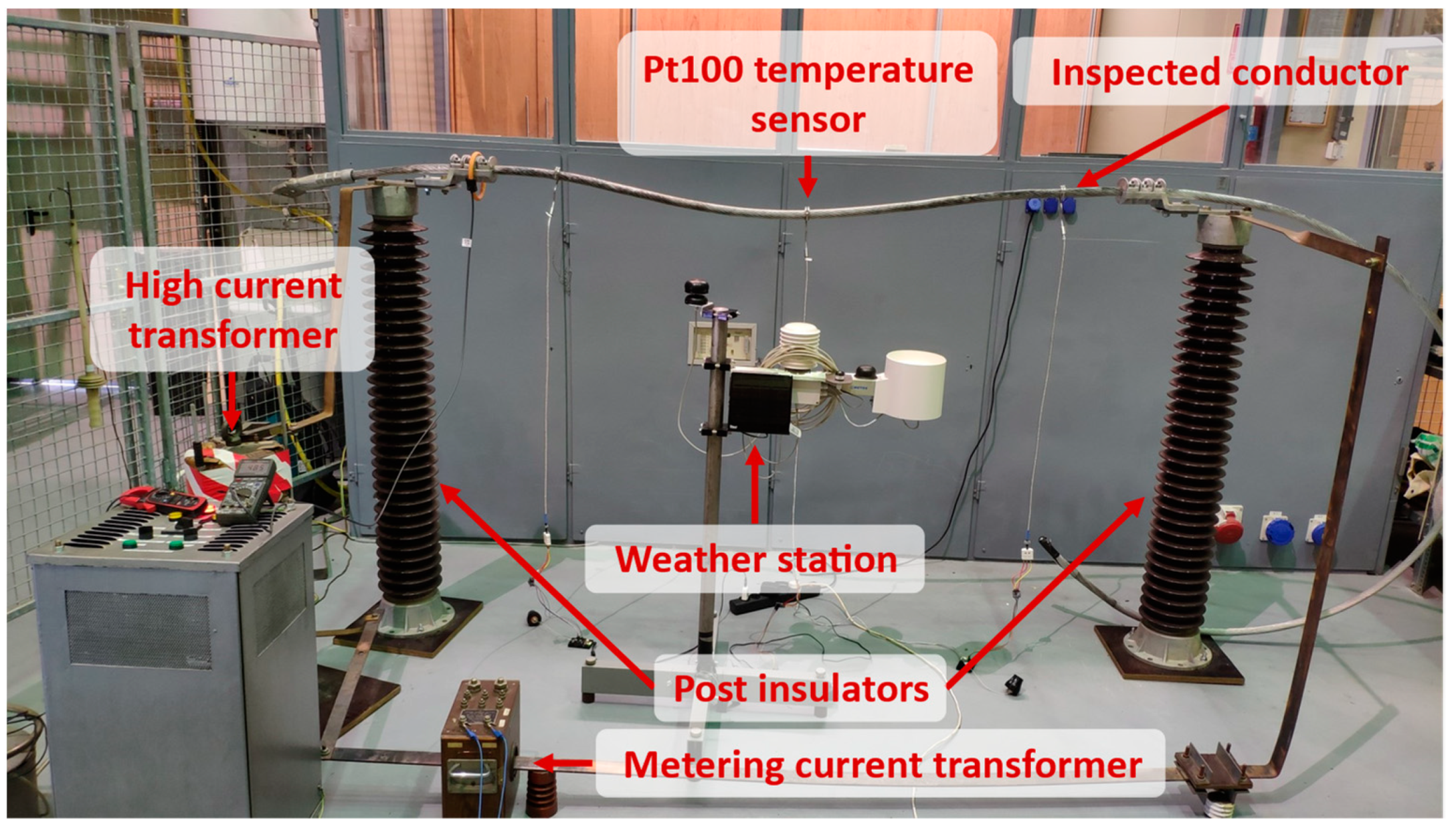
For the investigation of how accurate are in practice the existing international models and also the proposed one, which calculates the line rating in a direct way without the use of weather parameters, laboratory investigations have been carried out in the High Voltage Laboratory at the Budapest University of Technology and Economics. Both the ACSR 500/65 mm² and Hawk types of conductors have been tested, which were used in the previous sections for the comparison of the international calculation models. The 500/65 mm² ACSR conductor is provided by a Central European transmission system operator, which is commonly used on its 220 and 400 kV power lines. The Hawk type of conductor is supplied by a distribution system operator from another European country, which is commonly used in the 110 kV power lines across Europe.

During the laboratory inspections, a high current transformer is used as a power supply for the tested conductors, where the maximal ampere rating is 2000 A. For the supply of the high current transformer, a 0–400 V, 18 kVA adjustable toroid is used. The actual load of the inspected conductor is measured with a metering current transformer, where the ratio is 600:1 via a 6 ½ digit bench-top multimeter. The conductor temperature is measured with a 3-wire A-type of Pt100 sensor, which is designed for the measurement of the temperature of cylindrical surfaces. For the measurement of the environmental conditions, a weather station is applied. The accuracy of the measuring equipment is summarized in

Table 2. Measurement accuracy of the devices used during the laboratory tests.

Device		Resolution	Accuracy
6 ½ digit bench-top multimeter		6 ½ digit	±(0.23 + 0.04) 1
Pt100 temperature sensor		0.03 °C	±0.15 °C @ 0 °C ±0.35 °C @ 100 °C
Metering current transformer		n/a	class 1
Weather station	Temperature	0.1 °C	±1 °C
	Wind speed	0.05 m/s	±0.3 m/s
	Wind direction	1°	±3°
	Relative humidity	1%	±1%
	Solar radiation	n/a	±30 W/m2

¹ ± (% of reading + % of range).

.

The load of the conductor is measured every 5 s, the conductor temperature per minute and the weather parameters every 10 min. The measurement results of the current transformer are collected with the bench-top multimeter which is connected to a PC directly. Besides load current, the Pt100 sensor’s data are also collected in real time, which transferred to the PC via an online platform, and both data sources are processed with MATLAB R2022b. The measurements of the weather station are fetched retroactively from its online platform. The evaluation of the data and the calculation of the DLR values with the different models are also performed with the use of MATLAB R2022b software. The measurement arrangement is shown in Figure 5.

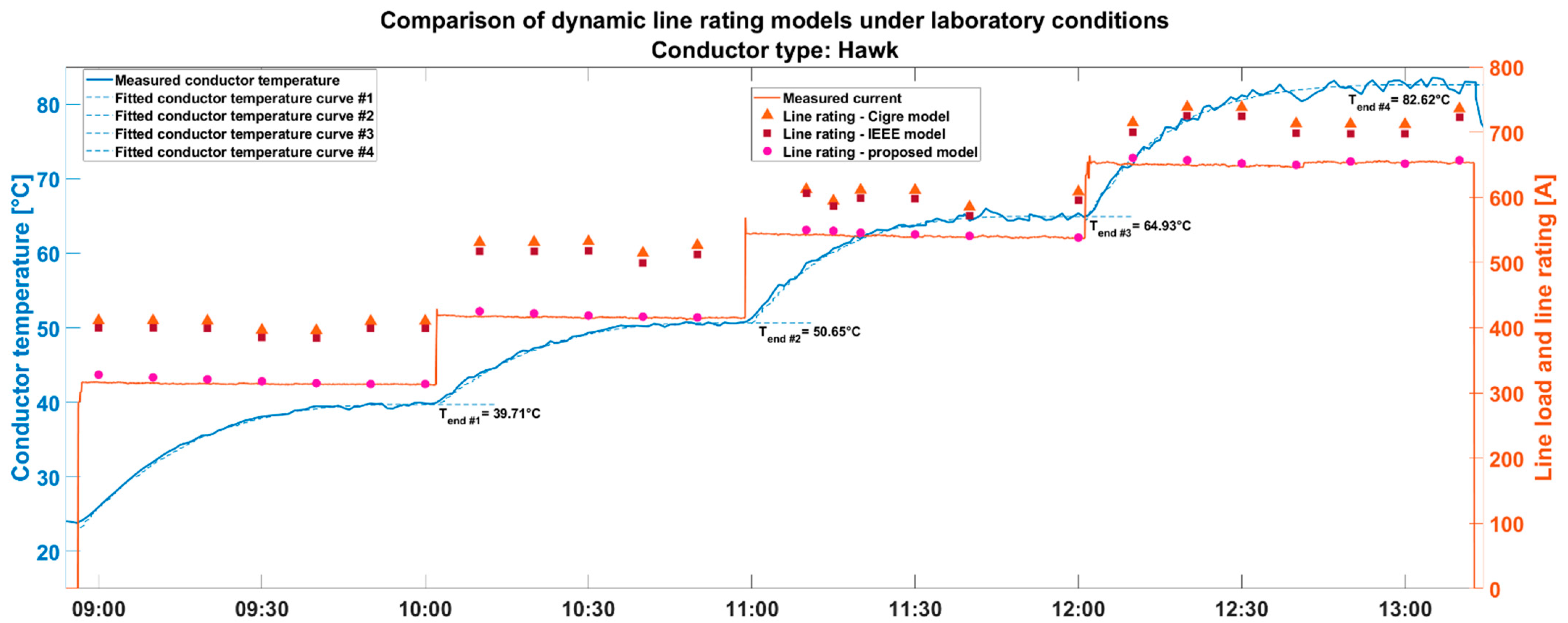
During the validation process, multi-step load values are applied to the inspected conductors, which means that a constant magnitude of current is applied for the time period until the conductor temperature is settled. The conductor temperature is considered as settled when it is not changed more than ±1 °C for a half-an-hour period. As the time constant of the Hawk conductor is less than the 500/65 mm² ACSR because of their different cross-sectional area, in the former case more load step values are applied. During each step, the line rating is calculated with the international models based on the environmental conditions measured by the weather station and the settled conductor temperature value. The final value of the conductor temperature of a given step is determined as the steady state value of the fitted curve on the conductor temperature measurements (dashed blue line in Figure 6 and Figure 7). For fitting the curve on the measured conductor temperature values, a two-term exponential curve is used. In the case of the proposed model, the line rating is determined based on the actually measured conductor temperature with the Pt100 sensor and the current flowing through the conductor.

The 4-step measurement of the Hawk type of conductor is shown in Figure 6.

In Figure 6, the accuracy of the different models can be interpreted visually as the deviation of the measured line load and the calculation results of a given model. This could be achieved because in each load step, the ampacity is calculated with the final value of the conductor temperature of the given step, which means the ampacity should be the measured line load in the given step. It can be seen in Figure 6 that the deviation of the international models is significantly greater than the proposed model. The main reason for the high deviation of the international models is that those models are based on the indirect measurement of the weather parameters and, e.g., the measurement accuracy of the weather station on the wind speed has a large effect on the calculated line rating. The proposed model is more and more accurate by reaching the steady-state value of the conductor temperature in a given step, which means that the local thermal overloads are completely avoided by applying the proposed model.

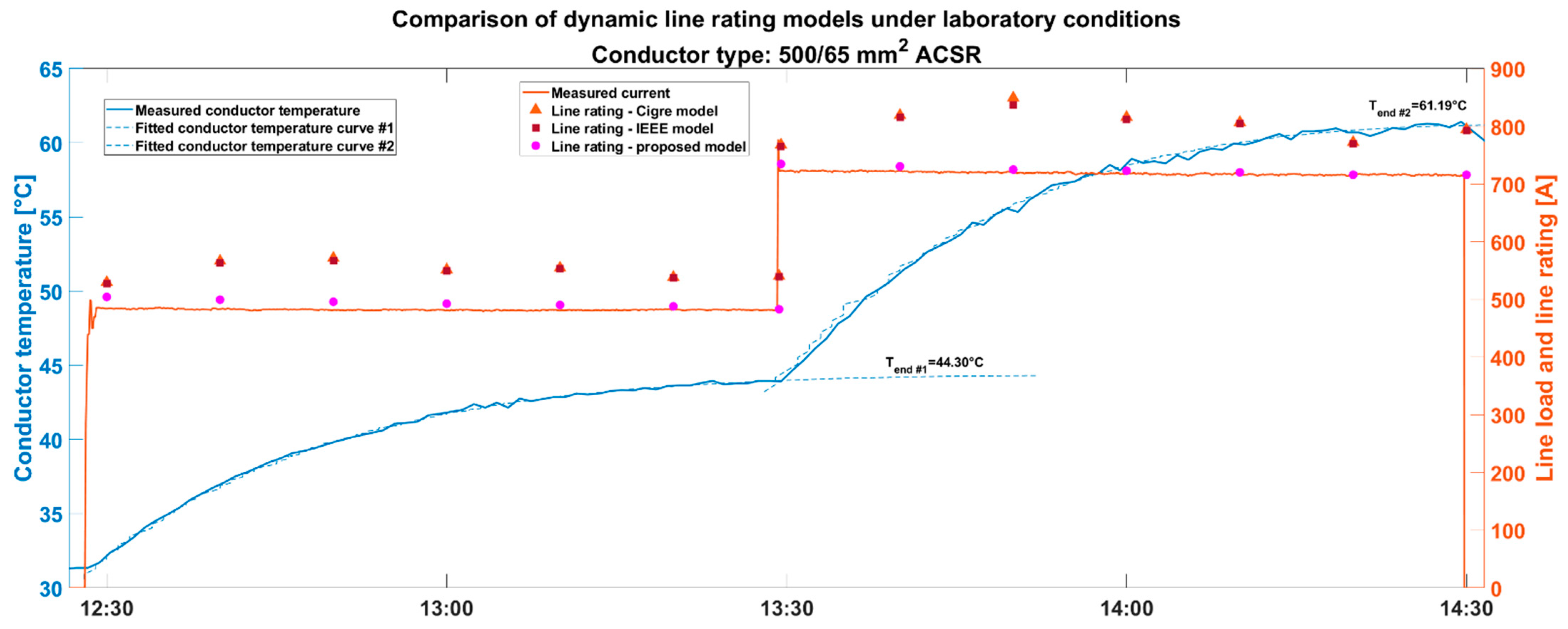
The same validation process results for the ACSR 500/65 mm² conductor are shown in Figure 7.

Regarding the tendencies, the validation process with the 500/65 mm² ACSR conductor shows the same results as in the case of the Hawk type of conductor, which is presented in Figure 7. It is also consistent in the measurements that the Cigre model overestimates the ampacity more than the IEEE one. For a more accurate evaluation of the validation laboratory measurements, a quantitative analysis is also performed for both laboratory measurements, which is summarized in

Table 3. Accuracy of the different line rating calculation models.

Model and Deviation in Line Rating [A/%]		Conductor/Load Step
		Hawk				ACSR 500/65 mm2
		#1 (310 A)	#2 (415 A)	#3 (540 A)	#4 (650 A)	#1 (480 A)	#2 (720 A)
Cigre	Min.	82.4 A/26.3%	100.2 A/24.2%	47.5 A/8.8%	59.6 A/9.1%	45.6 A/9.4%	45.8 A/6.3%
	Avg.	92.14 A/29.3%	112.4 A/27.1%	64.2 A/11.9%	73.5 A/11.3%	68.5 A/14.2%	85.5 A/11.9%
	Max.	96.9 A/30.9%	117.9 A/28.5%	72.2 A/13.4%	89.3 A/13.8%	89.9 A/18.7%	130.0 A/18.1%
IEEE	Min.	70.8 A/22.6%	85.2 A/20.6%	33.8 A/6.3%	44.9 A/6.9%	43.1 A/8.9%	42.6 A/5.9%
	Avg.	80.9 A/25.7%	98.1 A/23.6%	53.3 A/9.9%	59.3 A/9.1%	66.1 A/13.7%	81.3 A/11.3%
	Max.	85.8 A/27.4%	103.6 A/25.0%	64.2 A/11.8%	75.8 A/11.7%	84.8 A/17.6%	117.9 A/16.4%
Proposed	Min.	0 A/0%	2.5 A/0.6%	0 A/0%	1.7 A/0.3%	1.9 A/0.4%	0.7 A/0.1%
	Avg.	4.7 A/1.5%	5.0 A/1.2%	4.9 A/0.9%	4.7 A/0.7%	11.4 A/2.4%	5.4 A/0.8%
	Max.	11.8 A/3.8%	8.1 A/1.9%	8.2 A/1.5%	10.9 A/1.7%	20.2 A/4.1%	12.6 A/1.7%

.

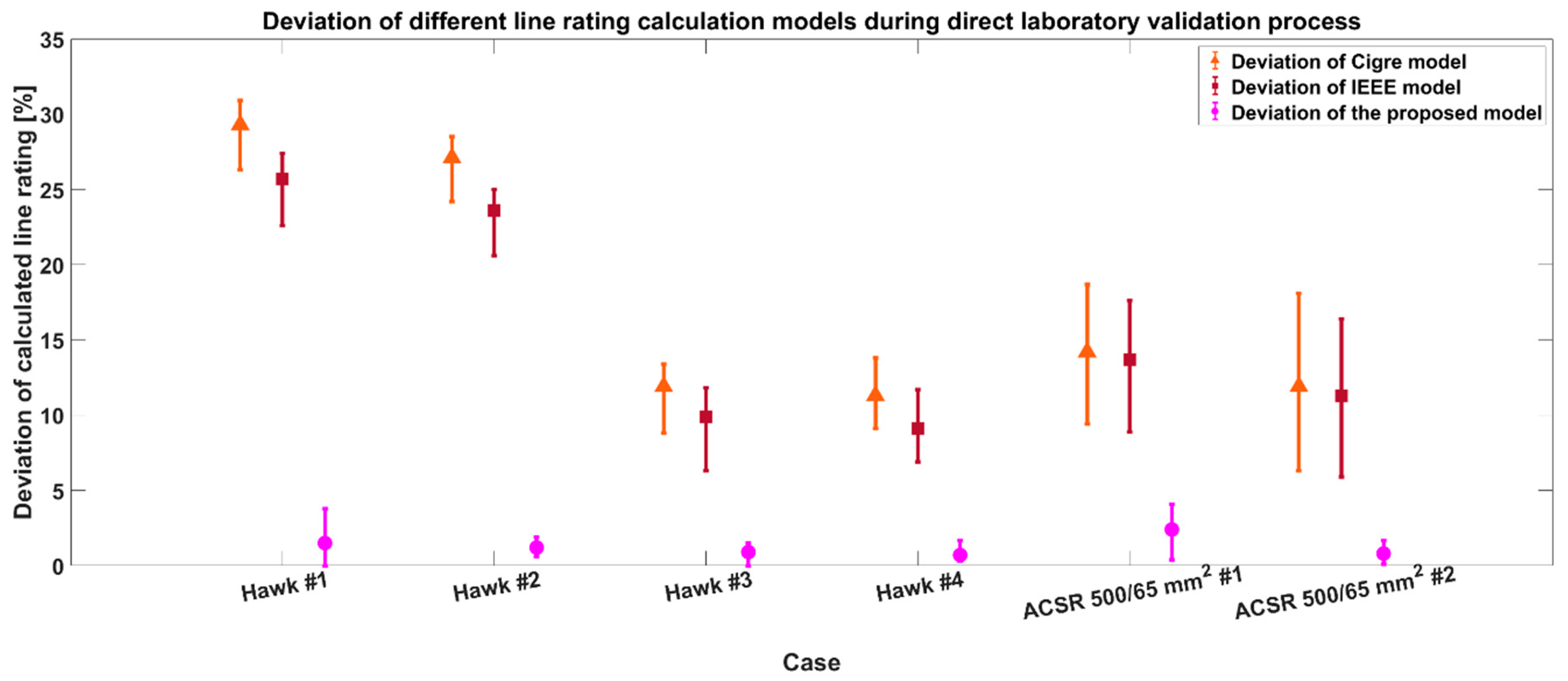
According to Table 3, it can be concluded that in the laboratory testing process—where the natural convection was dominant—all the models overestimated the real line rating. While in the case of the two international models the average overshot was higher than 10%, until then the proposed model overshot rate was below 2.5%. The model deviations are also presented in Figure 8.

All in all, the laboratory validation process showed that the proposed model provides much more reliable line rating results than the international models, which results in much less risk of the thermal overload of the conductors.

3.3. Case Study with the Proposed Model

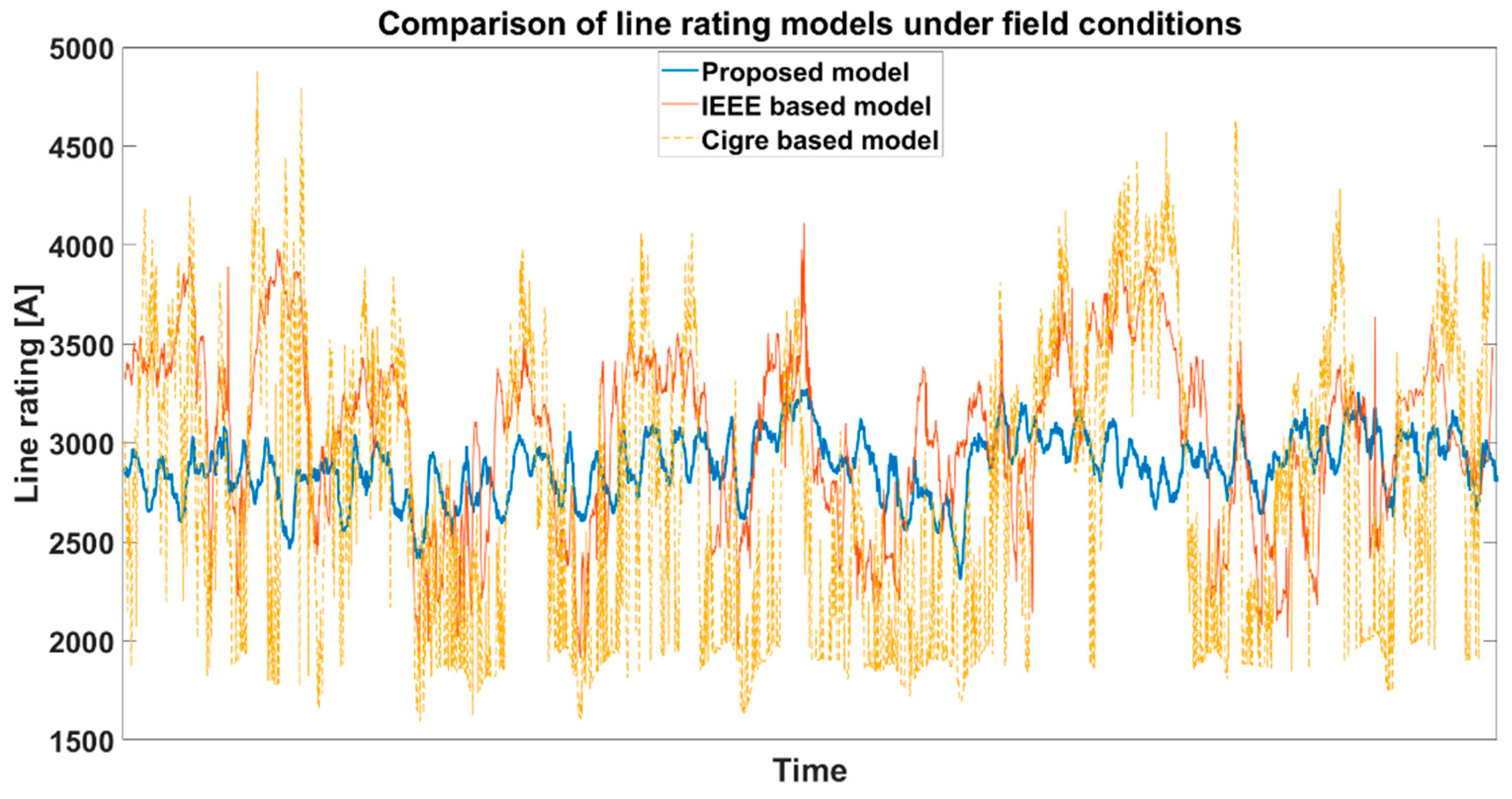
In order to achieve field experiences also, the proposed line rating calculation model is realized under the framework of the FARCROSS project at 4 European TSO’s sides. In this project, a weather station and two different line monitoring sensors are installed on the same span at each demonstration site. As one of the sensor manufacturers uses the IEEE while the other one uses the Cigre-based model for the DLR calculation, the proposed model had been compared with these calculation results under real field conditions. The results of the three different models for a one-month period are shown in Figure 9.

Figure 9 shows the biggest advantage of the proposed model from the practice point of view, which is that it has much smaller fluctuation than the weather-based models because the proposed model consists of the time constant of a given conductor. In practice, this means that the dispatchers can adapt more easily the less volatile transmission capacity constraints. On the other hand, the average capacity gain with the proposed model is in the same range as with the international ones, as summarized in

Table 4. Comparison of the line rating calculation models under field conditions.

Model	25th Percentile	Median	75th Percentile
Proposed model	2733 A	2870 A	2986 A
IEEE based model	2682 A	3108 A	3368 A
Cigre based model	2029 A	2762 A	3460 A

.

3.4. SWOT Analysis of the Proposed Model

In order to obtain a comprehensive picture of the advantages and disadvantages of the proposed dynamic line rating calculation method without weather parameters, a SWOT analysis have been performed.

The strength of the model is that it uses direct conductor temperature measurement in order to determine the line rating instead of the use of indirect weather parameters. As the line rating is determined by computing the difference in the actual conductor temperature and the maximal conductor temperature, the risk of thermal overload is negligible, which offers higher operational safety during the operation of the phase conductor at the maximal temperature. Moreover, the line rating calculated by the proposed model is less volatile, which supports the practical application of the DLR system, as the system operators have to adapt a less varying transfer capacity constraint in this way, reaching a more practical solution.

As the conventional DLR systems can be realized based on just the measurement of the environmental conditions, the actual conductor temperature is not known in all cases by the system operators. In contrast, the proposed model requires direct conductor temperature measurement, which contributes to the safer operation of the power lines, both from the point of view of ground clearance limitations and thermal aging of the conductors. Furthermore, the less varying dynamic transmission capacity constraint compared to the output of the conventional models allows the opportunity for the easier acceptance of the DLR technology from the user’s side.

The weakness of the proposed model is that it requires the direct measurement of the conductor temperature, which generally can be realized with more expensive field equipment than the measurement of the weather parameters in this way, leading to a more expensive system realization. Generally, it can be said that the capital expenditure of a DLR sensor is 1.5–2 times higher than a weather station. However, it should be highlighted that based on our experiences, the procurement of field equipment (DLR sensor and/or weather stations) means around the third part of the whole DLR system’s implementation cost. Accordingly, the use of DLR sensors instead of weather stations can increase the capital expenditure of a full DLR system realization by 10–30%.

The DLR system realized based on the proposed model has a threat also, namely that in the case of a sensor failure, the model input on that location cannot be substituted from another system or service. In the case of conventional models, the environmental conditions can be obtained from weather stations installed on the line or also from the nowcasting models of weather agencies, which offers a backup solution in case of the failure of field equipment. However, it should be noted that this threat concerns only the particular location of the failed sensors. As in a DLR system several sensors are installed on a line, the line rating can be determined with satisfying accuracy based on the measured data of other sensors in the case of a sensor failure during the reparation of the failed sensor.

Altogether, the explored strengths, weaknesses, opportunities and threats of the proposed model are summarized in

Table 5. SWOT analysis of the proposed line rating calculation model.

Strengths	Weaknesses
- Based on direct measurements - The risk of thermal overloads is negligible - Less volatile, more practical	- Requires more expensive sensors
Opportunities	Threats
- Direct feedback through conductor temperature measurement - Easier acceptance of DLR technology	- In case of a sensor failure, the model input cannot be substituted by weather agencies

.

4. Conclusions

The aim of this article was to present the development and validation process of a new dynamic line rating calculation methodology applied for the uprating of overhead lines. In the first part of the article, a literature overview was performed in order to review the so far existing dynamic line rating calculation methods. Moreover, the literature overview revealed the shortcomings of the international models, such as their inaccuracy, which can result in overshooting of the real ampacity or the volatility of the calculation results, which limits the practical application of the models. These all together provided the motivation for the development of a new way of thinking in the ampacity calculation.

In the second part of the article, a new dynamic line rating calculation model was proposed, which is based on the measurement of direct conductor temperature instead of the indirect measurement of the environmental factors. Firstly, the mathematical description of the ampacity calculation without weather parameters was described. In order to validate the model, laboratory measurements had been carried out, which not only evaluated the proposed model but also investigated the accuracy of the prevailing international models. Moreover, a case study was also presented to demonstrate how the proposed model can be applied in practice. Based on the so far existing experiences with the proposed model, it can be stated that it offers safer operation for the system operators. Thanks to the direct measurement of the conductor temperature, the risk of thermal overloads can be eliminated. Moreover, another advantage of the model is that the calculated ampacity is less varying in time due to the considered time constant of the conductors, which facilitates the practical application of the model.

The future plan of the authors is to test the proposed model on more sites in order to achieve further experiences with real field data. In this way, the calculation method can be fine-tuned, e.g., with the selection strategies of the calculation interval, and this way, the adjusted time constant of a given conductor type.