
Techno-Economic Comparison of Electricity Storage Options in a Fully Renewable Energy System


Abstract
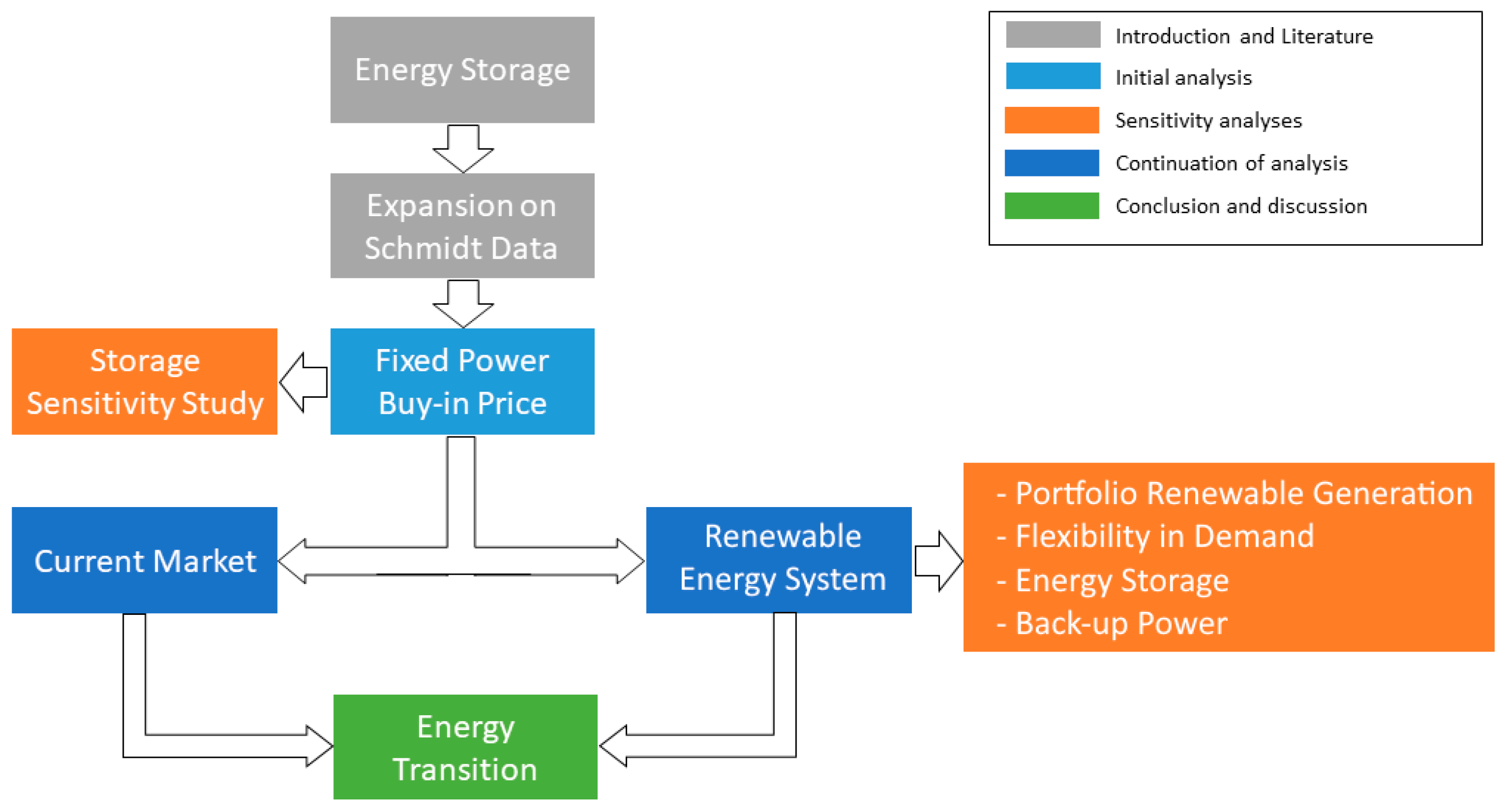
1. Introduction
2. Materials and Methods
2.1. LCOS Methodology
2.1.1. Capital Expenditure (CCAPEX)
2.1.2. Operations and Maintenance (COPEX)
End-of-Life (CEOL)
2.1.3. Charging Costs (Ccharge)
2.2. Description of Energy Storage Technologies
2.2.1. Lithium-Ion Battery (Li-Ion)
2.2.2. Sodium–Sulfur Battery (NaS)
2.2.3. Lead–Acid Battery (LeadAcid)
2.2.4. Vanadium Flow Battery (VaFlow)
2.2.5. Rankine-Type Thermal Energy Storage (RTES)
2.2.6. Pumped Thermal Energy Storage (PTES)
2.2.7. Pumped Hydro Storage (PHS)
2.2.8. Compressed Air Energy Storage (aCAES and dCAES-H2)
2.2.9. Liquid Air Energy Storage (LAES)
2.2.10. Hydrogen Gas Turbine (H2-CCGT)
2.2.11. Hydrogen Gas Turbine Retrofit (H2-CCGT-R)
2.2.12. Hydrogen Fuel Cell (H2-FuelCell)
2.3. Data Input to the Model
2.4. Geographical Restrictions
2.5. Part I: Comparison of Storage Technologies Using the Levelized Cost of Storage Methodology
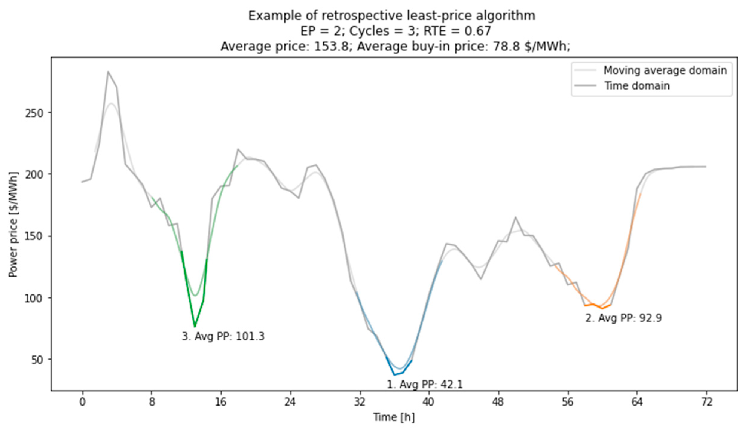
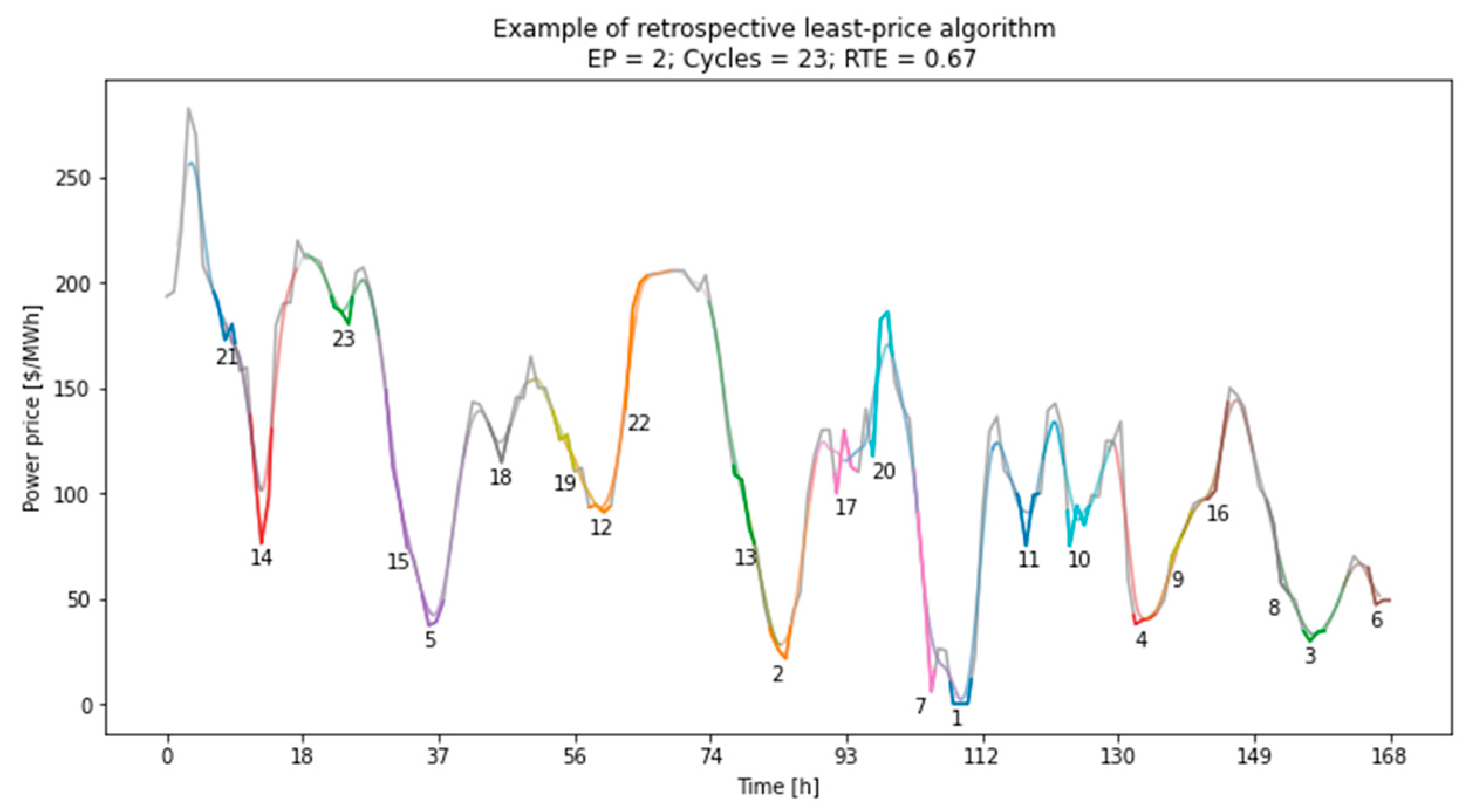
2.5.1. Fixed-Price Charging Cost Analysis
2.5.2. Charging of the Storage Based upon Market Power Prices
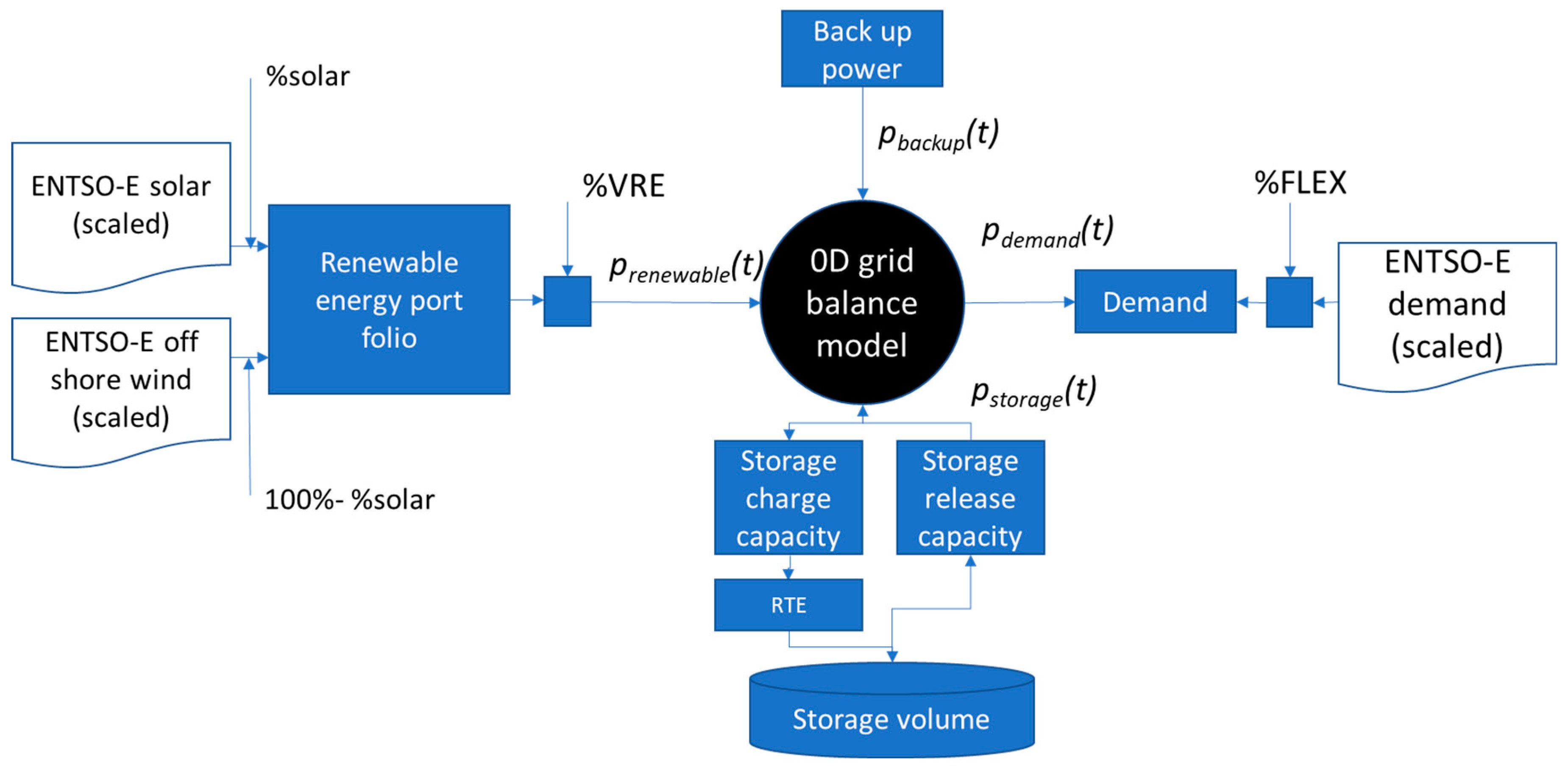
2.6. Part II: Energy Storage in a Fully Renewable Electricity System
- The generation of renewable electricity through solar PV and offshore wind.
- Demand, including flexibility in demand.
- Energy storage, as described in the first part of this paper.
- Backup power.
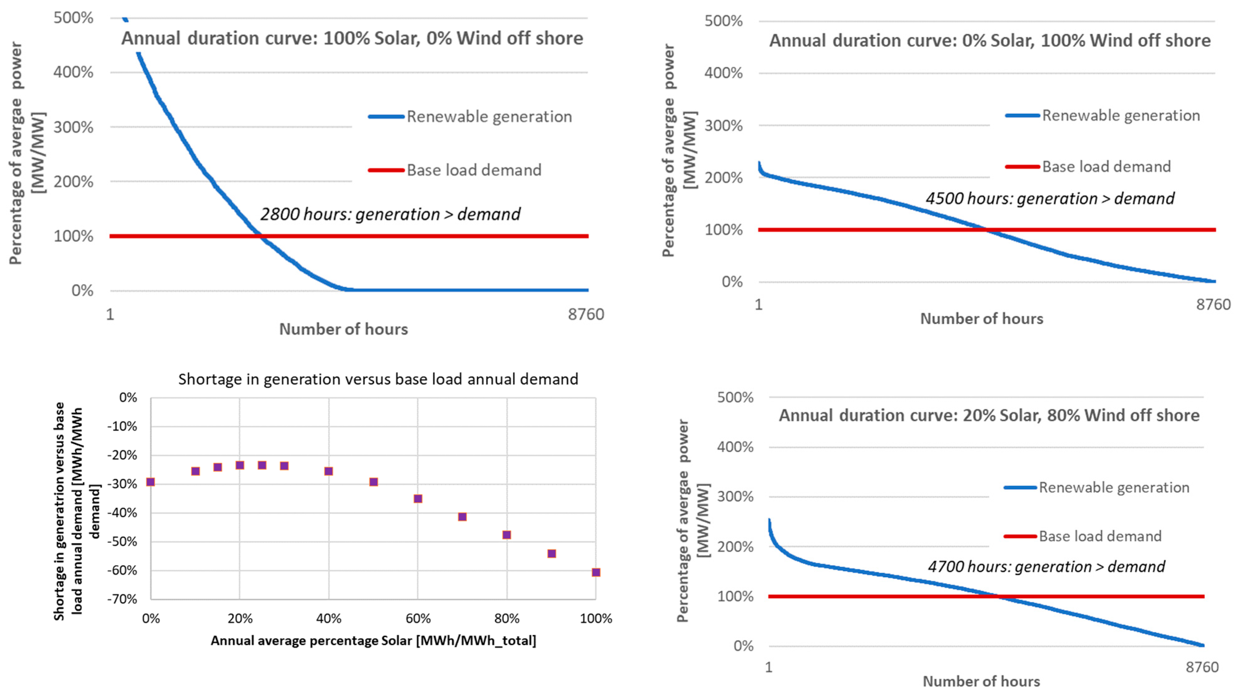
2.6.1. Portfolio of Renewable Generation
2.6.2. Methodology of the Renewable Energy System Study
- Energy generation at any hour is calculated using the renewable generation portfolio from the ENTSO-E data times a correction factor, %VRE.The %VRE is 100%, as the total annual generation (MWh) equals the total annual demand (MWh); a %VRE of 110% indicates a 10% excess in generation (MWh) versus the annual demand
- The balance between generation and demand is calculated for all hours.
- In case of unbalance in generation and demand, first storage is utilized:
- a.
- In case of an excess in generation, the excess generation for that hour is stored in the energy storage.
- b.
- In case of a shortage in generation, the shortage is delivered by the energy storage.
- c.
- The filling and releasing of the storage take place within the technical parameters:
- i.
- Round-trip efficiency.
- ii.
- Storage volume (in MWh, based upon release of electricity).
- iii.
- Storage capacity (both for intake of electricity and release of electricity).
- In case there is still a shortage in electricity at any hour, it is assumed that this electricity is generated by the backup power.In case there is still an excess in renewable production, it is assumed to be curtailed.
2.6.3. Optimal Levelized System Cost of Electricity for a Combined System of Renewable Generation and Storage
2.6.4. Optimization Procedure
3. Results
3.1. Part I: Comparison of Storage Technologies Using the Levelized Cost of Storage Methodology
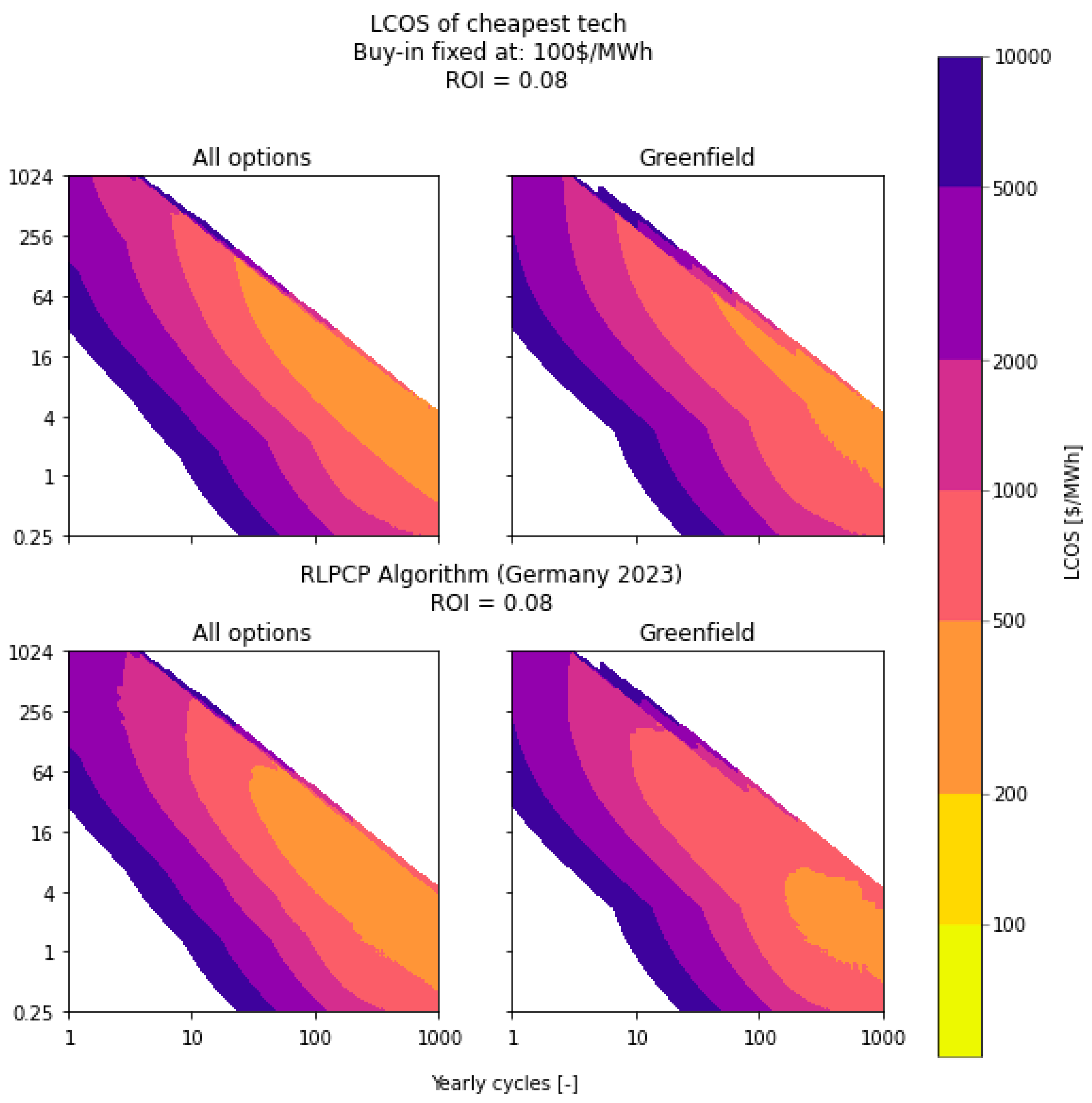
3.1.1. Fixed-Cost Analysis
3.1.2. Dynamic Price Analysis
3.2. Part II: Energy Storage in a Fully Renewable Electricity System
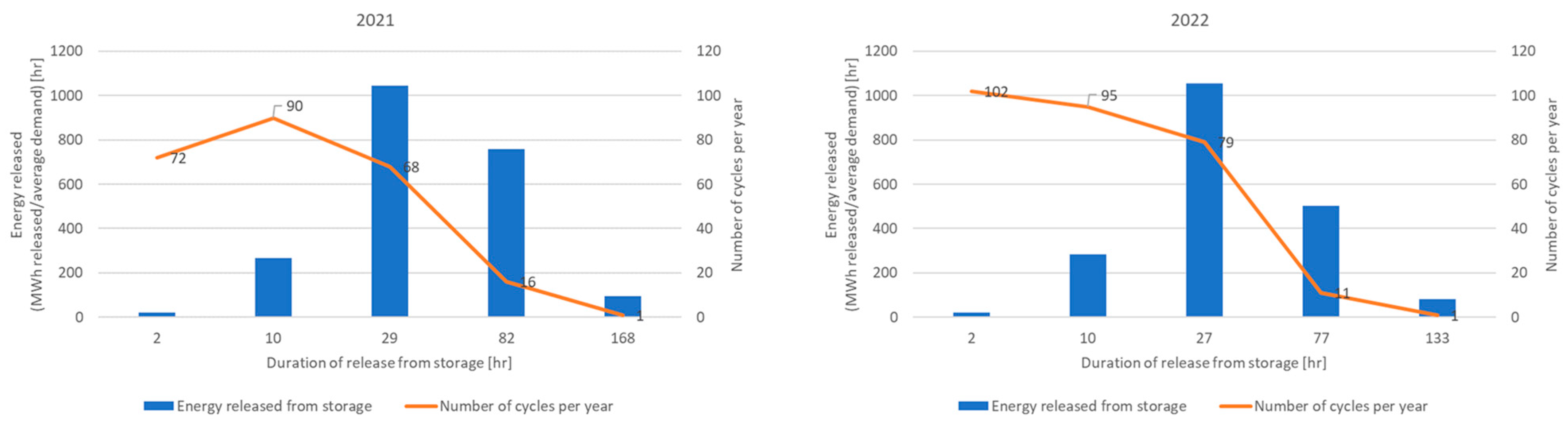
3.2.1. Time/Frequency Analysis of the Energy Balance in a 0D Grid Model
3.2.2. Comparison of LCOEsystem and LCOEstorage for Single Storage Technologies
3.2.3. Balance between Excess Renewable Generation Capacity and Storage Capacity
3.2.4. Sensitivity to Flexibility in Demand
4. Discussion
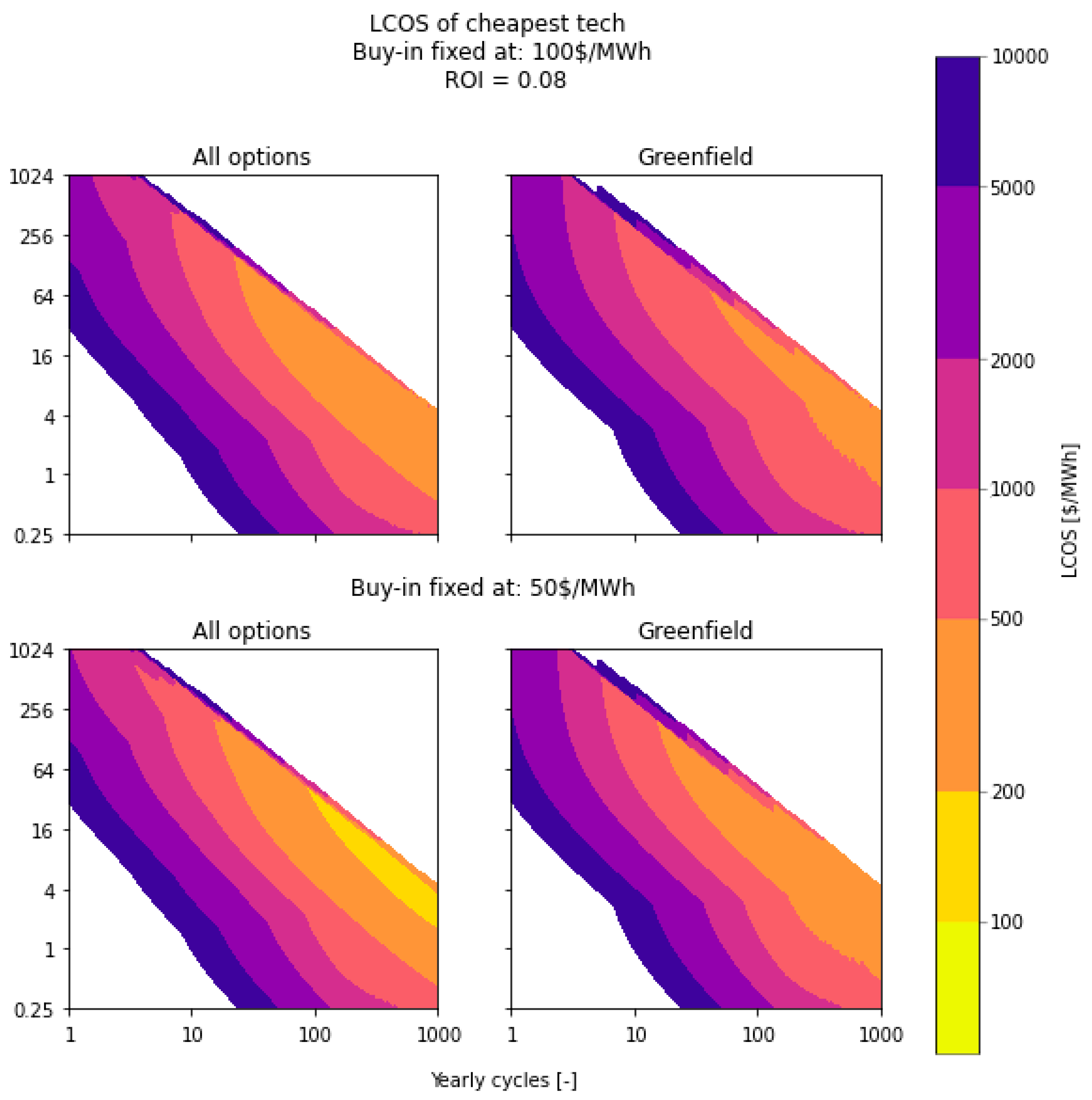
4.1. Impact of the Electricity Buy-In Price
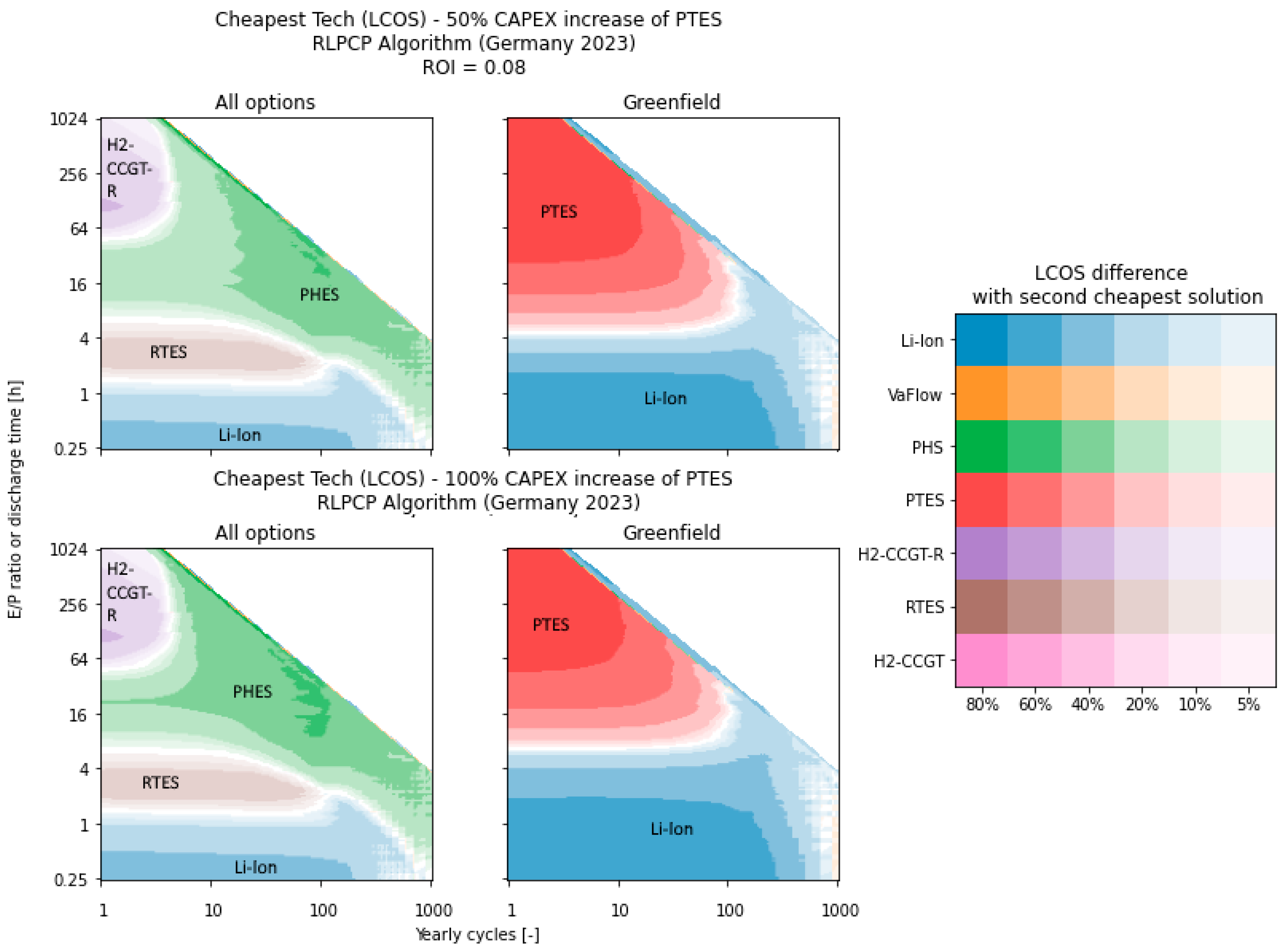
4.2. Influence of a Significant Reduction in CAPEX Costs on the Levelized Cost of Storage
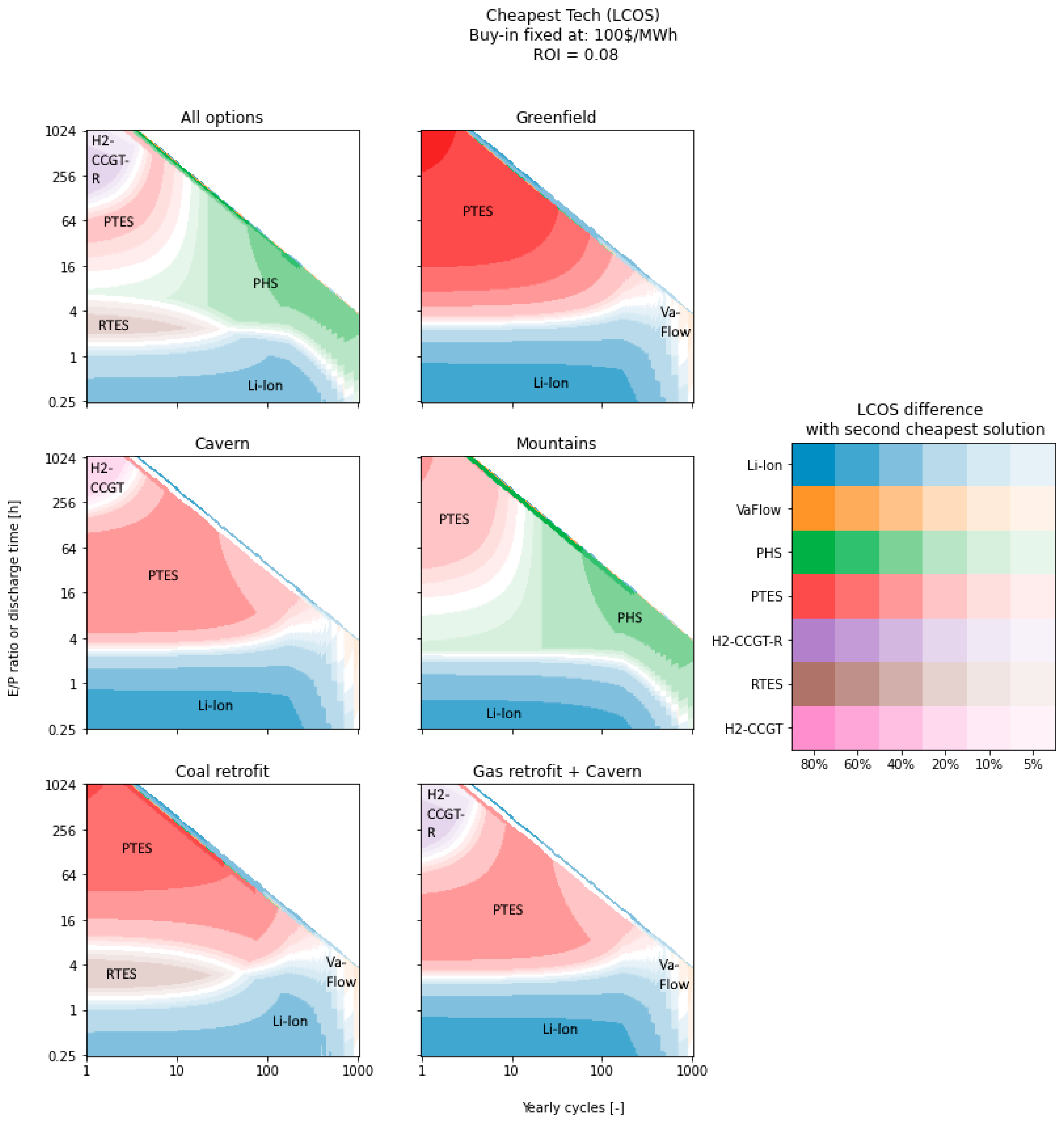
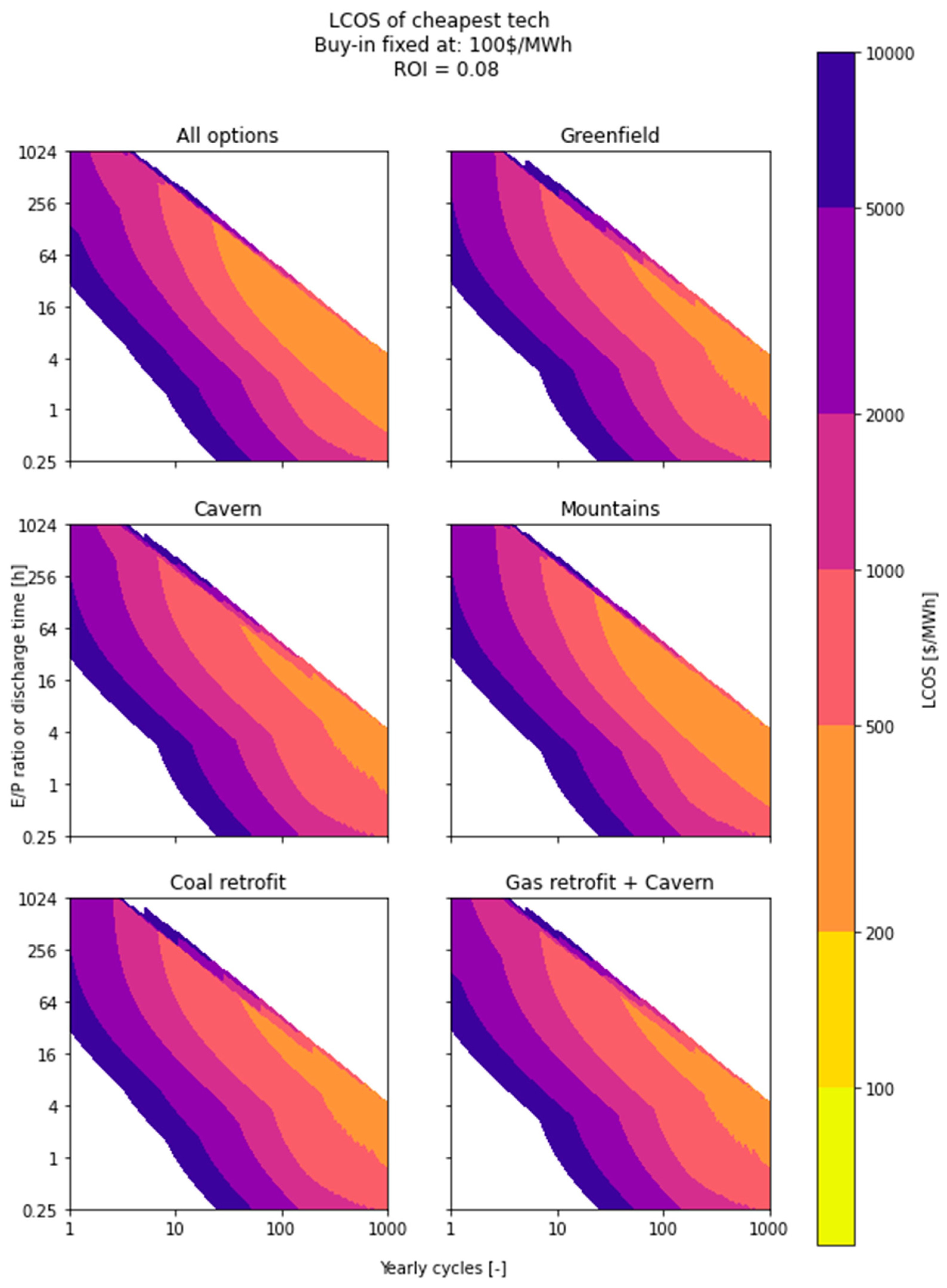
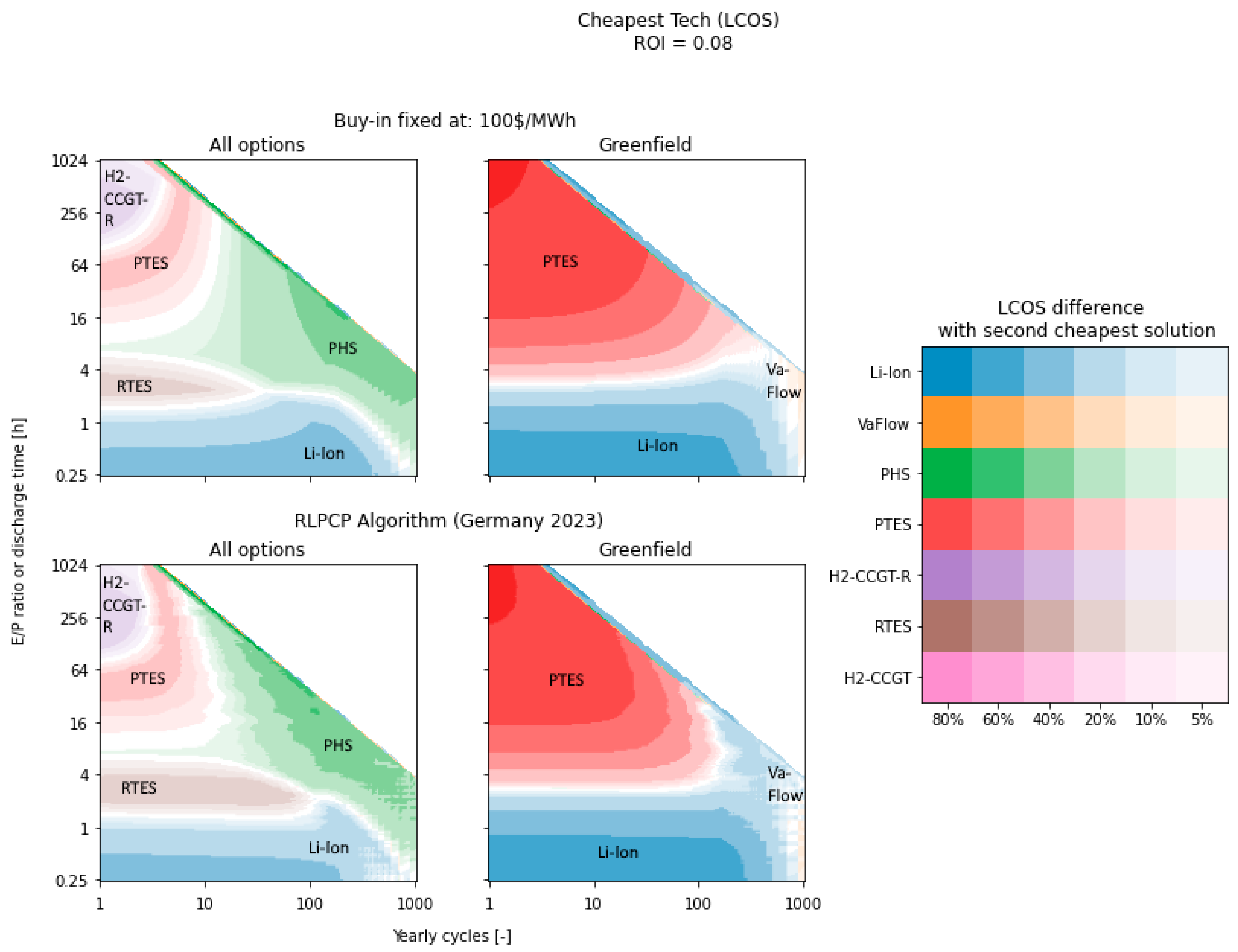
4.3. Second-Best Technologies for the Levelized Costs of Storage
4.4. Further Considerations
5. Conclusions
Author Contributions
Funding
Data Availability Statement
Conflicts of Interest
References
- Guarnieri, M.; Liserre, M.; Sauter, T.; Hung, J.Y. Future energy systems: Integrating renewable energy sources into the smart power grid through industrial electronics. IEEE Ind. Electron. Mag. 2010, 4, 18–37. [Google Scholar] [CrossRef]
- Ipakchi, A.; Albuyeh, F. Grid of the future. IEEE Power Energy Mag. 2009, 7, 52–62. [Google Scholar] [CrossRef]
- Bhatnagar, D.; Currier, A.; Hernandez, J.; Ma, O.; Kirby, B. Market and Policy Barriers to Energy Storage Deployment: A Study for the Energy Storage Systems Program. 2013. Available online: https://www.sandia.gov/ess-ssl/publications/SAND2013-7606.pdf (accessed on 23 February 2024).
- Jülch, V. Comparison of electricity storage options using levelized cost of storage (LCOS) method. Appl. Energy 2016, 183, 1594–1606. [Google Scholar] [CrossRef]
- Schmidt, O.; Melchior, S.; Hawkes, A.; Staffell, I. Projecting the Future Levelized Cost of Electricity Storage Technologies. Joule 2019, 3, 81–100. [Google Scholar] [CrossRef]
- Steckel, T.; Kendall, A.; Ambrose, H. Applying levelized cost of storage methodology to utility-scale second-life lithium-ion battery energy storage systems. Appl. Energy 2021, 300, 117309. [Google Scholar] [CrossRef]
- IEA. ETP Clean Energy Technology Guide; IEA: Paris, France, 2022. [Google Scholar]
- IEA. Grid-Scale Storage; IEA: Paris, France, 2022. [Google Scholar]
- Vistra. Morro Bay Energy Storage Project February 2021. 2021. Available online: https://www.morrobayca.gov/DocumentCenter/View/15093/Vistra---Morro-Bay---Battery-Project-Presentation-022021 (accessed on 21 September 2023).
- Cole, W.J.; Marcy, C.; Krishnan, V.K.; Margolis, R. Utility-scale lithium-ion storage cost projections for use in capacity expansion models. In Proceedings of the 2016 IEEE North American Power Symposium (NAPS), Denver, CO, USA, 18–20 September 2016; pp. 1–6. [Google Scholar] [CrossRef]
- Choi, D.; Shamim, N.; Crawford, A.; Huang, Q.; Vartanian, C.K.; Viswanathan, V.V.; Paiss, M.D.; Alam, M.J.E.; Reed, D.M.; Sprenkle, V.L. Li-ion battery technology for grid application. J. Power Sources 2021, 511, 230419. [Google Scholar] [CrossRef]
- Nitta, N.; Wu, F.; Lee, J.T.; Yushin, G. Li-ion battery materials: Present and future. Mater. Today 2015, 18, 252–264. [Google Scholar] [CrossRef]
- Zakeri, B.; Syri, S. Electrical energy storage systems: A comparative life cycle cost analysis. Renew. Sustain. Energy Rev. 2015, 42, 569–596. [Google Scholar] [CrossRef]
- Kumar, D.; Rajouria, S.K.; Kuhar, S.B.; Kanchan, D.K. Progress and prospects of sodium-sulfur batteries: A review. Solid State Ion. 2017, 312, 8–16. [Google Scholar] [CrossRef]
- McKeon, B.B.; Furukawa, J.; Fenstermacher, S. Advanced lead-acid batteries and the development of grid-scale energy storage systems. Proc. IEEE 2014, 102, 951–963. [Google Scholar] [CrossRef]
- Ding, C.; Zhang, H.; Li, X.; Liu, T.; Xing, F. Vanadium flow battery for energy storage: Prospects and challenges. J. Phys. Chem. Lett. 2013, 4, 1281–1294. [Google Scholar] [CrossRef]
- Zhang, H.; Lu, W.; Li, X. Progress and Perspectives of Flow Battery Technologies. Electrochem. Energy Rev. 2019, 2, 492–506. [Google Scholar] [CrossRef]
- Yong, Q.; Tian, Y.; Qian, X.; Li, X. Retrofitting coal-fired power plants for grid energy storage by coupling with thermal energy storage. Appl. Therm. Eng. 2022, 215, 119048. [Google Scholar] [CrossRef]
- Novotny, V.; Basta, V.; Smola, P.; Spale, J. Review of Carnot Battery Technology Commercial Development. Energies 2022, 15, 647. [Google Scholar] [CrossRef]
- Banaszkiewicz, M. Steam turbines start-ups. Trans. Inst. Fluid-Flow Mach. 2014, 126, 169–198. [Google Scholar]
- Cherif, S. Potential for Power-to-Heat in the Netherlands 3.E04.1-Potential for Power-to-Heat in the Netherlands. 2015. Available online: https://cedelft.eu/wp-content/uploads/sites/2/2021/04/CE_Delft_3E04_Potential_for_P2H_in_Netherlands_DEF.pdf (accessed on 23 February 2024).
- Laughlin, R.B. Pumped thermal grid storage with heat exchange. J. Renew. Sustain. Energy 2017, 9, 044103. [Google Scholar] [CrossRef]
- Smallbone, A.; Jülch, V.; Wardle, R.; Roskilly, A.P. Levelised Cost of Storage for Pumped Heat Energy Storage in comparison with other energy storage technologies. Energy Convers. Manag. 2017, 152, 221–228. [Google Scholar] [CrossRef]
- Rehman, S.; Al-Hadhrami, L.M.; Alam, M.M. Pumped hydro energy storage system: A technological review. Renew. Sustain. Energy Rev. 2015, 44, 586–598. [Google Scholar] [CrossRef]
- Zhou, Q.; Du, D.; Lu, C.; He, Q.; Liu, W. A review of thermal energy storage in compressed air energy storage system. Energy 2019, 188, 115993. [Google Scholar] [CrossRef]
- California Energy Commision. Pecho Energy Storage Center; California Energy Commision: Sacramento, CA, USA, 2021. [Google Scholar]
- Mongird, K.; Viswanathan, V.V.; Balducci, P.J.; Alam, M.J.E.; Fotedar, V.; Koritarov, V.S.; Hadjerioua, B. Energy Storage Technology and Cost Characterization Report. 2019. Available online: https://energystorage.pnnl.gov/pdf/PNNL-28866.pdf (accessed on 23 February 2024).
- Barbour, E. Thermodynamics of CAES. Energy Systems and Energy Storage Lab. 2014. Available online: http://www.eseslab.com/posts/blogPost_CAES_thermodynamics (accessed on 23 February 2024).
- Kim, J.; Noh, Y.; Chang, D. Storage system for distributed-energy generation using liquid air combined with liquefied natural gas. Appl. Energy 2018, 212, 1417–1432. [Google Scholar] [CrossRef]
- Guizzi, G.L.; Manno, M.; Tolomei, L.M.; Vitali, R.M. Thermodynamic analysis of a liquid air energy storage system. Energy 2015, 93, 1639–1647. [Google Scholar] [CrossRef]
- Vecchi, A.; Li, Y.; Ding, Y.; Mancarella, P.; Sciacovelli, A. Liquid air energy storage (LAES): A review on technology state-of-the-art, integration pathways and future perspectives. Adv. Appl. Energy 2021, 3, 100047. [Google Scholar] [CrossRef]
- Mongird, K.; Viswanathan, V.; Alam, J.; Vartanian, C.; Sprenkle, V.; Baxter, R. 2020 Grid Energy Storage Technology Cost and Performance Assessment. Energy 2020, 6–15. Available online: https://www.pnnl.gov/sites/default/files/media/file/Final%20-%20ESGC%20Cost%20Performance%20Report%2012-11-2020.pdf (accessed on 23 February 2024).
- Bouten, T.; Withag, J.; Axelsson, L.-U.; Koomen, J.; Jansen, D.; Stuttaford, P. Development and Atmospheric Testing of a High Hydrogen FlameSheetTM Combustor for the OP16 Gas Turbine. In Volume 3A: Combustion, Fuels, and Emissions; American Society of Mechanical Engineers: New York, NY, USA, 2021. [Google Scholar] [CrossRef]
- Lazard. Levelized Cost of Energy+. 2023. Available online: https://www.lazard.com/research-insights/levelized-cost-of-energyplus/ (accessed on 23 February 2024).
- Schoenfisch, M.; Dasgupta, A. Grid-Scale Energy Storage. 2022. Available online: https://www.iea.org/energy-system/electricity/grid-scale-storage (accessed on 23 February 2024).
- Frauenhofer ISE. Monthly Electricity Spot Market Prices in Germany in September 2023. Available online: https://energy-charts.info/charts/price_average/chart.htm?chartColumnSorting=default (accessed on 24 September 2023).
- ENTSO-E. ENTSO-E Transparancy Platform. 2020. Available online: https://transparency.entsoe.eu// (accessed on 15 November 2023).
- Hirth, L.; Mühlenpfordt, J.; Bulkeley, M. The ENTSO-E Transparency Platform—A review of Europe’s most ambitious electricity data platform. Appl. Energy 2018, 225, 1054–1067. [Google Scholar] [CrossRef]
- Bernath, C.; Deac, G.; Sensfuß, F. Impact of sector coupling on the market value of renewable energies—A model-based scenario analysis. Appl. Energy 2021, 281, 115985. [Google Scholar] [CrossRef]
- Bogdanov, D.; Ram, M.; Aghahosseini, A.; Gulagi, A.; Oyewo, A.S.; Child, M.; Caldera, U.; Sadovskaia, K.; Farfan, J.; Barbosa, L.D.S.N.S.; et al. Low-cost renewable electricity as the key driver of the global energy transition towards sustainability. Energy 2021, 227, 120467. [Google Scholar] [CrossRef]
- Schmidt, O. System Integration of Low-Carbon Electricity. 2023. Available online: https://www.storage-lab.com/emission-mitigation (accessed on 21 September 2023).
- Heide, D.; von Bremen, L.; Greiner, M.; Hoffmann, C.; Speckmann, M.; Bofinger, S. Seasonal optimal mix of wind and solar power in a future, highly renewable Europe. Renew. Energy 2010, 35, 2483–2489. [Google Scholar] [CrossRef]
- Sens, L.; Neuling, U.; Kaltschmitt, M. Capital expenditure and levelized cost of electricity of photovoltaic plants and wind turbines—Development by 2050. Renew Energy 2022, 185, 525–537. [Google Scholar] [CrossRef]
- Heffron, R.; Körner, M.F.; Wagner, J.; Weibelzahl, M.; Fridgen, G. Industrial demand-side flexibility: A key element of a just energy transition and industrial development. Appl. Energy 2020, 269, 115026. [Google Scholar] [CrossRef]
- Zhang, L.; Sun, C.; Cai, G.; Koh, L.H. Charging and discharging optimization strategy for electric vehicles considering elasticity demand response. eTransportation 2023, 18, 100262. [Google Scholar] [CrossRef]
- Cole, W.; Karmakar, A. Cost Projections for Utility-Scale Battery Storage: 2023 Update; NREL: Golden, CO, USA, 2023. [Google Scholar]
- Schmidt, O.; Staffel, I. Monetizing Energy Storage, 1st ed.; Oxford University Press: Oxford, UK, 2023. [Google Scholar]


| Li-Ion | NaS | LeadAcid | VaFlow | PTES | aLAES | RTES | PHS | aCAES | dCAES-H2 | H2-CCGT | H2-CCGT-R | H2-FuelCell | |
|---|---|---|---|---|---|---|---|---|---|---|---|---|---|
| CAPEX (USD/kW) | 250 a | 650 a | 300 a | 700 a | 797 b | 2000 c | 300 | 1100 a | 980 d | 1230 d | 1600 d | 980 d | 2050 e |
| CAPEX (USD/kWh) | 300 a | 450 a | 320 a | 450 a | 21 b | 500 c | 63 | 50 a | 30 d | 3 d,e | 3 d,e | 3 d,e | 3 d,e |
| CAPEX Factor (-) | 1 | 1 | 1 | 1 | 1 | 1 | 1 | 1 | 1.25 d | 1 | 1 | 1 | 1 |
| OPEX (USD/MWh) | 0.4 a | 0.4 a | 0.4 a | 2 a | 2.6 d | 2.6 d | 2.6 d | 0.4 a | 2.6 d | 3.3 d | 3 d | 3 d | 3 d |
| OPEX (USD/kW-y) | 5 a | 5 a | 5 a | 10 a | 11 d | 11 d | 11 d | 11 d | 11 d | 14.9 d | 3.2 e | 3.2 | 28.5 e |
| Replacement (USD/kW) | 50 a | - | - | 90 a | - | - | - | 120 a | 100 a | 100 a | - | - | - |
| Replacement (USD/kWh) | 150 a | - | - | 0 a | - | - | - | 0 a | 0 a | 0 a | - | - | - |
| Rep. Interval (103) | 3.5 a | - | - | 3.5 a | - | - | - | 7.3 a | 1.5 a | 1.5 a | - | - | - |
| EoL (USD/kW) | 0 a | 20 a | 20 a | 20 a | 20 a | 20 a | 20 a | 20 a | 20 a | 20 a | 20 a | 20 a | 20 a |
| EoL (USD/kWh) | 20 a | 0 a | 0 a | −100 a | 0 a | 0 a | 0 a | 0 a | 0 a | 0 a | 0 a | 0 a | 0 a |
| RTE (-) | 86% a | 75% a | 72% a | 68% a | 57.5% b | 49.3% c | 41.8% | 80% a | 70% d | 55% d | 41% d | 41% d | 35% e |
| DoD (-) | 80% a | 80% a | 80% a | 100% a | 100% | 100% | 100% | 100% a | 100% a | 63% d | 63% d | 63% d | 63% d |
| Self-Discharge (1/c) | 1% a | 5% a | 1% a | - | 2% b | 1% b | 2% b | - | 0.75% d | 0% d | 0% d | 0% d | 0% d |
| Cycle Life (103 cycles) | 3.5 a | 4 a | 0.9 a | 20 a | 14.6 b | 10 a | 10 a | 30 a | 15 a | 15 a | 10 a | 10 a | 10 a |
| Shelf Life (y) | 20 | 15 a | 10 a | 20 a | 20 b | 20 d | 30 d | 80 d | 35 d | 35 d | 30 d | 30 d | 30 e |
| Degradation (1/y) | 1% a | 1% a | 1% a | 0.15% a | - | - | - | - | - | - | - | - | - |
| End-of-Life (-) | 80%a | 80% a | 80% a | 95% a | 80% | 95% | 95% | 95% a | 95% a | 95% a | 95% a | 95% a | 95% a |
| Construction Time (y) | 1 a | 1 a | 1 a | 1 a | 1 | 1 | 1 | 3 a | 2 a | 2 a | 2 a | 2 a | 1 |
| Li-ion | NaS | LeadAcid | VaFlow | PTES | aLAES | RTES | PHS | aCAES | dCAES-H2 | H2-CCGT | H2-CCGT-R | H2-FuelCell | |
|---|---|---|---|---|---|---|---|---|---|---|---|---|---|
| All options | |||||||||||||
| Greenfield | |||||||||||||
| Cavern | |||||||||||||
| Mountains | |||||||||||||
| Coal retrofit | |||||||||||||
| Gas retrofit |
| Offshore Wind | Solar PV | |
|---|---|---|
| CAPEX (USD/kW) | 2000 | 400 |
| Annual O&M costs | 2.5% | 1.3% |
| Optimization Parameter | Min. | Max. | |
|---|---|---|---|
| %VRE | 100% | 150% | Given as a percentage of annual average demand |
| Intake capacity of storage | 0.1% | 100% | |
| Release capacity of storage | 0.1% | 100% | |
| Volume of storage | 1 h | 200 h | Multiplied by the annual average hourly demand |
| E/P Ratio (h) | 2 | 10 | 24 | 93 | 133 |
|---|---|---|---|---|---|
| Yearly Cycles (-) | 81 | 111 | 90 | 5 | 1 |
| Li-Ion | 944 | 657 | 825 | ||
| NaS | 2429 | 1382 | 1640 | ||
| LeadAcid | 2575 | 2960 | |||
| VaFlow | 1816 | 1015 | 1228 | ||
| PTES | 1152 | 562 | 731 | 1449 | 5433 |
| dLAES | 3922 | 1442 | 1509 | ||
| RTES | 848 | 962 | 1378 | 3689 | |
| PHS | 1018 | 330 | 385 | 1708 | 7489 |
| aCAES | 2001 | 699 | 838 | 2630 | |
| dCAES-H2 | 2591 | 1088 | 1400 | 3037 | |
| H2-CCGT | 1818 | 2177 | 2481 | 6377 | |
| H2-FuelCell | 2662 | 3120 | 3634 | 9426 | |
| H2-CCGT-R | 2552 | 1585 | 2069 | 1928 | 4442 |
| E/P Ratio (h) | 2 | 10 | 24 | 93 | 133 |
|---|---|---|---|---|---|
| Yearly Cycles (-) | 81 | 111 | 90 | 5 | 1 |
| Li-Ion | 950 | 518 | 563 | ||
| NaS | 2437 | 1168 | 1237 | ||
| LeadAcid | 2387 | 2599 | |||
| VaFlow | 1822 | 817 | 855 | ||
| PTES | 1142 | 201 | 121 | 1191 | 5369 |
| dLAES | 3930 | 1317 | 1251 | ||
| RTES | 797 | 229 | 202 | 3174 | |
| PHS | 1023 | 195 | 130 | 1592 | 7459 |
| aCAES | 1992 | 356 | 220 | 2364 | |
| dCAES-H2 | 2570 | 443 | 262 | 2584 | |
| H2-CCGT | 609 | 293 | 1650 | 6104 | |
| H2-FuelCell | 942 | 494 | 2461 | 8977 | |
| H2-CCGT-R | 2470 | 376 | 185 | 1096 | 4170 |
Disclaimer/Publisher’s Note: The statements, opinions and data contained in all publications are solely those of the individual author(s) and contributor(s) and not of MDPI and/or the editor(s). MDPI and/or the editor(s) disclaim responsibility for any injury to people or property resulting from any ideas, methods, instructions or products referred to in the content. |
© 2024 by the authors. Licensee MDPI, Basel, Switzerland. This article is an open access article distributed under the terms and conditions of the Creative Commons Attribution (CC BY) license (https://creativecommons.org/licenses/by/4.0/).
Share and Cite
Mulder, S.; Klein, S. Techno-Economic Comparison of Electricity Storage Options in a Fully Renewable Energy System. Energies 2024, 17, 1084. https://doi.org/10.3390/en17051084
Mulder S, Klein S. Techno-Economic Comparison of Electricity Storage Options in a Fully Renewable Energy System. Energies. 2024; 17(5):1084. https://doi.org/10.3390/en17051084
Chicago/Turabian StyleMulder, Sebastiaan, and Sikke Klein. 2024. "Techno-Economic Comparison of Electricity Storage Options in a Fully Renewable Energy System" Energies 17, no. 5: 1084. https://doi.org/10.3390/en17051084
APA StyleMulder, S., & Klein, S. (2024). Techno-Economic Comparison of Electricity Storage Options in a Fully Renewable Energy System. Energies, 17(5), 1084. https://doi.org/10.3390/en17051084