Article

CFD Simulation Models and Diffusion Models for Predicting Carbon Dioxide Plumes following Tank and Pipeline Ruptures—Laboratory Test and a Real-World Case Study

1
School of Engineering, University of St. Thomas, St. Paul, MN 55105, USA
2
Institute of Atmospheric Physics, Chinese Academy of Sciences, Beijing 100029, China
*
Author to whom correspondence should be addressed.
Energies 2024, 17(5), 1079; https://doi.org/10.3390/en17051079
Submission received: 6 February 2024 / Revised: 19 February 2024 / Accepted: 19 February 2024 / Published: 23 February 2024
(This article belongs to the Section B3: Carbon Emission and Utilization)

Abstract

:
Ruptures of pipelines can result in dangerous fluids spreading toward populated areas. It is critical for designers to have tools that can accurately predict whether populated areas might be within a plume rupture zone. Numerical simulations using computational fluid dynamics (CFD) are compared here with experimental and real-world carbon dioxide ruptures. The experimental data were used to validate the computer model; subsequently, the algorithm was used for a real-world rupture from 2020 that occurred in the USA. From experiments, CFD predictions were superior to diffusion model results based on measurements made downstream of the release (within 1% concentration). Results from the real-world simulation confirm that a nearby town was in a plume pathway. Citizens in the town sought medical attention consistent with the calculated plume concentrations. CFD predictions of the airborne concentration of carbon dioxide in the town approximately 1 mile (1.5 km) downstream of the rupture reveal time-averaged concentrations of ~5%. One person was unconscious for ~45 min at a distance of 0.6 miles from the rupture site; other unconscious persons were in the center of the town (~1 mile from the rupture site) and ~1.2 miles from the rupture. These reports are in excellent agreement with the calculated plume concentrations in the region.

1. Introduction

One of the most pressing challenges to today’s global society is climate change and its nexus to energy. That climate change is happening is undisputed (as described in refs. [1,2,3,4], for example, with measurements of global warming rates). The only remaining scientific questions deal with the rate and overall extent of the changes.
In response to climate change, various approaches have been proposed for reducing atmospheric greenhouse gases and collecting carbon dioxide from production locations. Once collected, CO2 can be used for various industrial purposes and/or stored underground, a process referred to as carbon capture and storage (CCS).
The transport of CO2 can be performed with pipeline networks—pipelines are generally more cost-effective than other modes of transport, but pipelines have their drawbacks. Among these are the potential ruptures of pipelines and storage vessels. Following a rupture, cold, high-pressure media are released into the atmosphere and then travel as a plume in the direction of prevailing winds.
Concentrations of 0.5% are permissible for 8 h exposures for workplaces in the USA as representative of levels that might be a concern for populated areas. Concentrations of 1% can cause drowsiness, while 1.5% concentrations lead to mild respiratory systems [5]. With concentrations of 3%, more severe respiratory effects occur, whereas at 4%, a plume causes a risk of death if exposure is sufficiently long. A more exhaustive discussion of CO2 health impacts can be found in [6,7]; interested readers are directed there. Of course, health impacts also depend on the exposure duration and any complicating health factors that may be present. The very high pressures and volumes involved in ruptures can result in large areas that are affected. Because of this, it is essential to carry out risk assessments for areas near pressurized CO2 pipelines or vessels. In essence, this requires calculating the area impacted by a plume.
There are two typical means of calculating plume impact areas. The first method is called dispersion modeling—a technique based on simplified diffusion zones of uniform or assumed concentration profiles that move in the direction of the prevailing wind and involve plumes spreading transverse to the wind. Another approach is termed computational fluid dynamics (CFD), a technique that solves the conservation of mass, momentum, and energy at many computational elements (a computational mesh). While more complex, CFD calculations can be more accurate because they account for the local motion of the atmosphere. Because of its simplicity, plume dispersion modeling is more commonly used in industry applications; however, both approaches have a role in risk assessment. In this study, the ability of CFD to perform plume calculations will be explored. First, calculations will be performed for multiple test cases. Next, CFD will be applied to a real-world rupture that occurred in 2020 in the USA.
This study is novel because it involves the application of CFD to both laboratory-scale and real world-scale problems. Furthermore, to the best of our knowledge, it is the first CFD model of a real-world pipeline rupture that involves complicated terrain and weather information. In addition, the results of the real-world model are compared with reports of persons seeking medical attention following the rupture.
CFD can be used while pipeline routes are being planned to reduce the risk to communities if a rupture was to occur. For example, results from CFD can identify what weather conditions and rupture locations present a danger to a given region. As another use, the results of CFD calculations can be used to more safely route pipelines to reduce risk. In addition, CFD calculations can help quantify regions that are affected following a rupture.
That said, CFD calculations typically require too much time to provide real-time plume locations; therefore, CFD calculations should be performed before a rupture. This confirmatory information is valuable because large, full-scale ruptures are not expected. This study will demonstrate that commercially available fluid flow software can adequately quantify the impact area of a plume and the concentrations of a gas species within the plume.

2. Background on Dispersion Modeling and CFD

Dispersion modeling (sometimes alternatively referred to as unified dispersion modeling (UDM) or a Gaussian model) is a mature and easy-to-use approach ([8,9]). There are multiple versions of dispersion programs, and the PHAST approach will be used as a representative. Other dispersion codes include ALOHA, CANARY, SLAB [10], HEGADAS [11], DEGADIS [12], and FRED, among others [13]. There are slight variations in the approaches used by dispersion/Gaussian models, but in short, they assume a concentration profile in an affected region, and the size and position of the profile are governed by nearby conditions such as wind speed, turbulence level, and local temperature, among others. Hereafter, these groups will be referred to collectively as “dispersion models” or UDMs, even though some algorithms do not require a uniform concentration.
UDMs can incorporate either instantaneous or prolonged ruptures from pressurized or unpressurized sources, and they have varying levels of sophistication. One of the most commonly encountered models is PHAST, but many others also exist, as will be described later. To the authors’ best knowledge, the first comprehensive presentation of the PHAST algorithm was provided by [14] along with a very detailed description of its implementation. As discussed there, UDM models incorporate both near-field and far-field dispersion. A rupture often involves the release of very high-pressure gas that rapidly cools because of the Joule–Thomson effect. The rapid temperature and pressure changes in the medium lead to various phase changes (gas–liquid–solid). The dispersion plume is presumed to possess a concentration profile that has either sharp-edge boundaries or a Gaussian profile. The models allow for the sublimation of solid into vapor near the rupture location and the possibility of rainout and re-evaporation, mass transfer between the plume and the ground, and ground-to-plume heat transfer. Despite the ability of PHAST and other UDMs to incorporate many features, the basis for the calculations are assumptions of the concentration profiles, and those assumptions are often not met in the real world.
The thermodynamics associated with high-pressure releases can be complex; however, often, the fluid is supercritical in the storage vessel. Following rupture, the plume is generally near the triple point. The plume exponentially decays in the transverse directions with dispersion coefficients that have been obtained from wind tunnel experiments. Depending on the release direction, the plume is ejected into the ambient air and then—after its momentum is expended—falls to the ground as it continues to spread. The plume descent results from the density difference between the cold plume and the adjacent air. Additionally, there is a difference in the molecular masses between CO2 and air (nitrogen and oxygen).
The dispersion model enforces a plume shape that is typically circular until the plume reaches the ground, after which it is a truncated circular cross-section. As the plume travels downstream, it entrains nearby air, affecting the spread and mass within it. Entrainment also adds turbulence to the plume—at the interface between the fast-moving plume and the slower-moving ambient. Further mixing is caused by the background turbulence levels in the atmosphere, heat transfer from the ground, and momentum conservation in the transverse directions. In some cases, atmospheric instability, such as rising buoyant convective cells, can enhance mixing. In fact, generally, more stable atmospheric conditions enable plumes to travel further distances than less stable conditions allow.
Dispersion models presume a spatial shape of a concentration plume with distribution functions, such as a Gaussian, used to capture variations in concentration transverse to the prevailing winds. As an example, the form of the model used by the ALOHA UDM is represented as follows (x is the wind direction dimension):
C x , y , z = σ 2 π σ z σ y V w i n d e 1 2 y σ y 2 · e 1 2 z z o σ z 2 + e 1 2 z + z o σ z 2
where the σ terms represent standard deviation in the horizontal crosswind direction (y) and the vertical direction (z).
While diffusion models have some minor differences, their core calculations are similar. For example, the PHAST diffusion model calculates a spatially varying concentration from the following:
C x , y , z = C o x · e y R y n · e z R z m
Ry and Rz are the dispersion coefficients in the y and z directions, respectively. Values of n and m control the sharpness of the plume boundary with the adjacent fresh air. For values n = m = 2, the profiles are Gaussian; as n and m values increase beyond 2, the profile edges become increasingly sharp. The values of the parameters in Equations (1) and (2) are based on calibration studies with laboratory experiments.
As reported in [14], the PHAST UDM model was applied to various gas plumes, and a comparison between calculations and experiments was provided. With respect to CO2, it was found that at a distance of 640 m from a rupture, PHAST underpredicted experimental concentrations by 393%, a surprisingly large discrepancy for a controlled test over flat ground. Other validation tests were performed with sulfur dioxide, ammonia, propane, Freon, LNG, and HF. Some of the validation work was not published because of a confidentiality agreement, but the published works show mixed performance for PHAST.
Another UDM study was published [15] that focused on the discharge and thermodynamics of the near-field plume. While the discussion of near-field thermodynamics is helpful, the study itself is not dispositive because of the paucity of downstream data. More recently, the same team published a validation of PHAST against experimental observations [16] using both steady-state releases (DISC) and time-varying releases (TVDI). Those test cases were small scale (less than 100 m) in length. Sublimation between solid and gaseous phases was assumed to be very rapid so that only a vapor plume occurred.
While the number of factors that can be accounted for with UDM is extensive, there are some significant weaknesses with the UDM approach. First, concentration profiles are assumed and correlated to match wind tunnel experiments. The circular cross-sectional shape of the plume is also assumed. While convenient for simplicity, there is no physical basis to support this assumption. Furthermore, UDM models cannot handle non-flat terrain or obstacles (buildings, trees, etc.). In addition, UDM models cannot account for spatial or temporal variations in the local wind speed. Finally, UDM models have a mixed record of accuracy when compared to real-world situations. In some cases, UDM calculations have vastly underpredicted plume travel. Additionally, UDMs generally assume plume travel in the prevailing wind direction—something that may or may not occur [16]. Notably, attempts to connect dispersion models to 2D ground flow models (designed for liquid spills) are not relevant for gaseous and vapor flow.
Generally, PHAST studies do not provide much information about validation because of the confidential information of the measurements. However, ref. [16] provided some experimental data that is useful for model development. Additionally, ref. [17] compared CFD to PHAST calculations and found that the results were not very sensitive to the particle sizes at the rupture site (solid CO2 from Joule–Thomson cooling). Concentration predictions were lower using PHAST than a CFD model (ANSYS CFX).
Bayesian analysis was combined with PHAST by [18]. That study identified the most important input parameters to a UDM analysis and included limited CFD calculations using ANSYS CFX. Later, ref. [19] considered both PHAST and CFD and found that CFD was superior to PHAST modeling. Studies [20,21] continued the comparison of PHAST and CFD and noted that “In general, CFD models are the most adaptable and can produce better predictions as they use more detailed mathematical descriptions of the conservation principles. This allows simulation of complex physical processes involving heat and mass transport in complicated computational domains”. These include various source terms to account for atmospheric stability [22]—a study that accurately used CFD to predict concentration plumes ~1000 m downstream of a release.
The studies in refs. [20,21] relied upon 1995 CO2 experiments (Kit Fox experiments) that were carried out in Nevada, USA. The solution domain extended 225 m downstream of the release location. The authors concluded that CFD performs well in both flat and complex terrain situations and “perform much better than the Gaussian and similar-profile model SLAB”. Other studies that have looked at the ability of dispersion and CFD models to calculate plumes include [23,24,25]. Generally, they found that obstructions and terrain are important factors and that CFD is more capable of predicting plumes than other approaches. These studies also found that multiple turbulence closure models can provide accurate results. These findings reinforce earlier results that found dispersion models incapable of calculating the flow over obstacles or with spatial/temporal variations in weather conditions [26]. It is noteworthy that [20] recommended using CFD models to train less sophisticated dispersion models. Additional studies have been performed on the impact of shrubbery and the ability of CFD models to account for this factor ([27]) as well as other terrain complexities [28,29]. As stated already, these factors are important to plume trajectory [23]. Ref. [30] was a follow-up study that confirmed the ability of CFD to calculate CO2 plumes in areas with obstacles during a full-scale test. Their results provide more evidence supporting the use of CFD calculations for these problems.
In the context of prior research, it is an open question whether the simplicity and ease of use of simple dispersion models provide more value than more complex and more accurate CFD models. Is either approach preferred? Are these approaches exclusive or complementary? Finally, are CFD codes too onerous for their routine use in CCS situations? Answers to these questions will be useful for risk assessment in the real world and are, thus, the focus of the present research. Additionally, data from a real-world unintentional rupture are missing from the literature; to the best of the authors’ knowledge, the present study is the first to use CFD for predicting plume motion in such a situation.
There is a body of helpful literature that interested readers are directed to—these studies are not particularly germane to the findings of the present study but nevertheless provide a detailed collective overview of this subject [20,31,32,33,34,35,36,37,38]. Other studies discuss the origination and development of different dispersion models that readers are directed to [39,40]. Very recent publications include [41], where a review of dispersion modeling was provided. Additionally, ref. [42] used PHAST for a case study that involved natural gas leakage near a population center. Still, this publication did not include experimental measurements, and, thus, its value is limited. Diffusion modeling was used to simulate release from an ethylene tank in [43] from an explosive rupture. More recent efforts to combine flow models with artificial intelligence have appeared and have promise; however, AI–flow model combinations are not yet deployed for real-world use [44,45] and other approaches, such as large eddy simulation (LES) for both large-scale [46] and small-scale problems [47] are currently limited. Despite these prior studies, to the authors’ best knowledge, there are no full-scale real-world CFD calculations of CO2 dispersion (or other gaseous components) following a rupture.

3. CFD Modeling of Plumes

3.1. Governing Equations

CFD relies upon the solution of fundamental equations throughout the solution domain; equations governing the conservation of mass, momentum, concentration, and energy are required. When multiple species are involved, the bulk motion of the mixture is solved with singular values of pressure, temperature, and velocity. However, each species has separate conservation of mass. This study has two species (air and carbon dioxide). While air is technically a mixture of primarily N2 and O2, treating it as a single species with properties that reflect the mixture is standard. The conservation of mass for species i is expressed as follows:
ρ i t + ρ i u j x j = ρ i u i j u j ρ i u j ¯ x j
In this equation, ρi is the average mass density of the ith fluid component in the mixture; the subscript i refers to the ith component, and the subscript j refers to a tensor direction. The uj term is the mass average velocity in the j direction. Equation (3), when applied to both components in the mixture, becomes the following:
ρ i t + ρ i u j x j = 0
The relative motion of the two species may be different because of diffusion effects (driven by concentration gradients), and the governing diffusion equation is the following:
ρ i u i j u j = D i ρ i x j
The symbol Di is the kinematic diffusivity of species i. The multi-component specific concentration equations are solved as a scalar transport equation with the mass fraction ϕ as the variable. The resulting transport equation is the following:
ρ ϕ i t + ρ ϕ i u i x j = D i ϕ i x j x j ρ ϕ i u i x j ¯
The differential transport of a species is reproduced using an eddy dissipation approximation with a turbulent Schmidt number so that the species transport equation can be rewritten as follows:
ρ ϕ i t + ρ ϕ i u i x j = D e f f ϕ i x j x j
The term Deff includes both molecular and turbulent diffusion. The other constraint in a multi-component system is that the sum of all mass fractions must equal one.
The conservation of momentum is written as follows:
ρ u j t + u i u j x i = p x i + x i μ + μ t u j x i j = 1 , 2 , 3
In these equations, x indicates a tensor-based direction, and u represents mixture velocities in the x, y, and z directions. The symbols ρ, μ, p, and μτ are density, molecular viscosity, pressure, and eddy viscosity, respectively. Concerning thermal energy, the governing equation is provided in enthalpy form as follows:
ρ h t p t + ρ u j h x j = x j k k c p + μ t P r t u r b h x j  
Enthalpy terms, h, are mass-weighted averages of the two species. All local fluid properties are calculated using the results from the energy equation—fluid properties such as density require temperature information. More details of the multi-component species transport equations can be found in [48] and a portion of this discussion has been paraphrased from that source.
Turbulence is dealt with using the shear stress transport model, which is a two-equation turbulence model based on turbulent kinetic energy (k) and the specific rate of turbulence dissipation (w). The turbulence equations are the following:
  ρ k t + ρ u i k x i = P k β 1 ρ k ω + x i μ + μ t u r b σ k k x i
ρ ω t + ρ u i ω x i = α 3 ω κ P κ β 2 ρ ω 2 + x i μ + μ t u r b σ ω ω x i + 2 1 F 1 ρ 1 σ ω 2 ω k x i ω x i
and the turbulent viscosity is found from the following:
μ t = a ρ k m a x a ω , S F 2
Pk is the production of turbulent kinetic energy and ω reflects the specific rate of turbulent destruction. As noted earlier, the σ terms are turbulent Prandtl numbers associated with their subscript. The function F1 is the aforementioned blending function that transfers the k-ω model near the wall to the k-ε model away from the wall. The S term is the magnitude of the shear strain rate.
Solutions to the energy equations are important to quantify buoyancy. The buoyancy model is the Boussinesq approach [49]. Buoyant forces in the vertical direction are quantified by a pseudo density difference that is related to temperature within the gas compared to a reference temperature To, so that the following is true:
ρ ρ o = α · T o T
The symbols ρo and To are reference density and temperature, while α is the thermal expansion of the fluid with temperature. With this approximation, the buoyant force in the vertical direction is calculated. In addition, turbulent fluid motion affects the eddy viscosity, which, in turn, impacts the contribution of turbulent motion to the thermal conductivity and the diffusivity. Consequently, the conservation of mass, momentum, energy, and species are solved simultaneously. It is noted that both species (CO2 and air) were modeled using their respective ideal gas laws so that the effects of temperature and pressure are incorporated into the buoyancy forces.
Interested readers are invited to read [50,51,52,53] for more information about the underlying code. For dealing with turbulence, the shear stress transport model was used [54] because of its demonstrated record of solving similar problems. The shear stress model is characterized as a Reynolds-averaged Navier–Stokes (RANS) approach that averages small-scale turbulent fluctuations. We also refer readers to [55,56,57,58], which articulate some recent and relevant advances in modeling that are related to multi-phase buoyant flows.

3.2. Validation

The first calculations correspond to validation exercises that will be used to determine if the CFD model can provide sufficiently accurate solutions for plumes. In this regard, calibration is based on [16] and is a horizontal release of CO2. Two tests from [16] were used (Tests 9 and 11); the input parameters are listed in Table 1.
Figure 1 shows the geometry of the validation tests. The solution domain extended 200 m in the flow direction (175 m downstream of the horizontal injection location). The transverse size of the solution domain was 150 m, and the height of the domain was 25 m. Boundary conditions are annotated in Figure 2. A no-slip condition was applied with a smooth surface on the ground. The top surface and the sides are openings that enable air to flow into and out of the domain based on entrainment. The release was positioned 0.5 m above the ground.
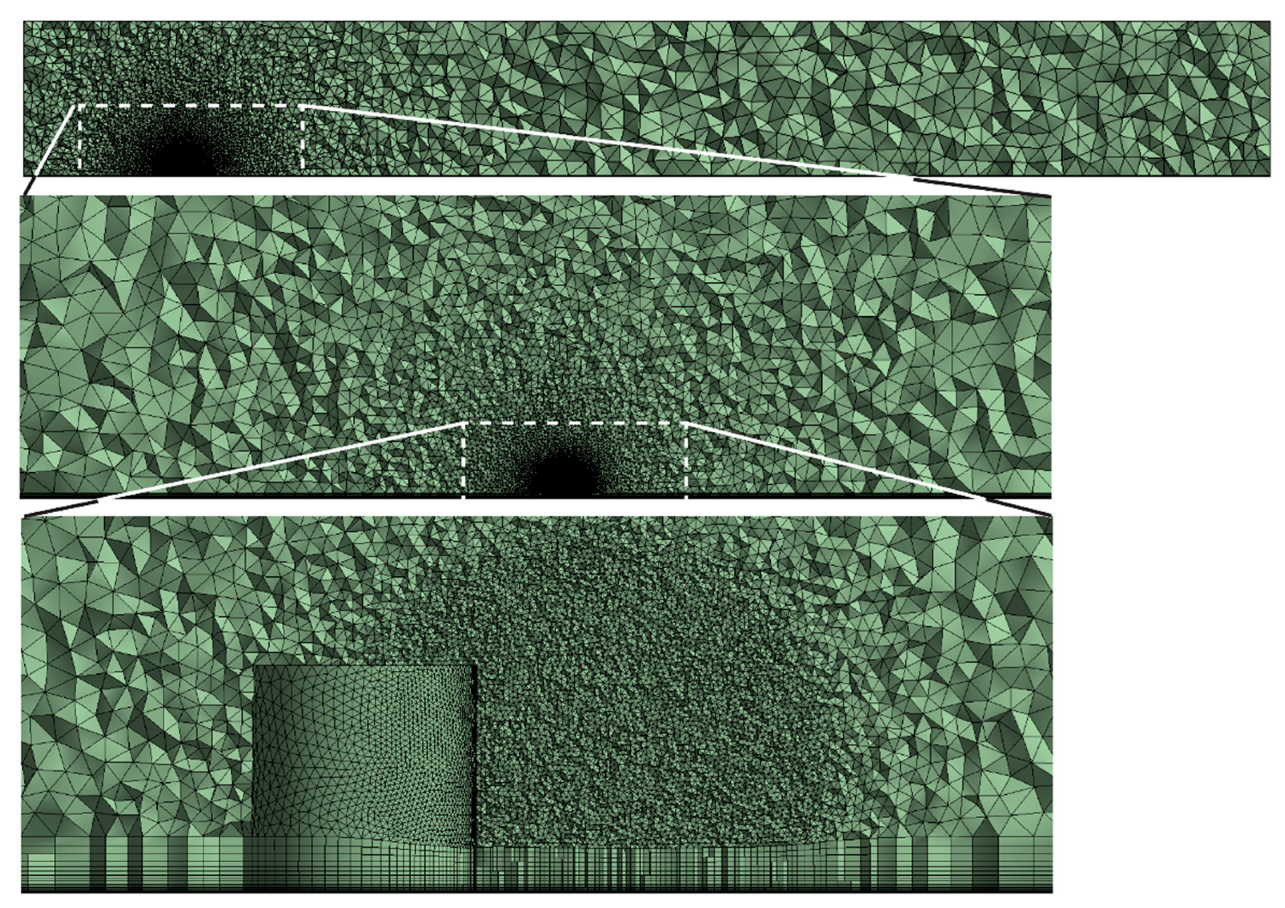
The quality of the computational mesh can be important for numerical accuracy. Images of the mesh are shown in Figure 2. The images show sequentially closer views of the mesh, focusing on the release location. Near the ground, particularly evident in the bottommost figure, are special boundary layer elements. These computational elements promote the accurate calculation of airflow in the boundary layer. The release was from a short vertical extension that is visible in the lowermost figure. The release surface shape is circular. The white lines are used to show subsequent enlarged images.
The mesh was subjected to a mesh-independence study wherein the elements were made progressively smaller until the calculations no longer changed. The final mesh utilized for the validation study incorporated 3.7 million elements. Buoyancy was included in the analysis with a gravitational acceleration of 9.8 m/s2. Both production and dissipation of turbulence by buoyancy were allowed, and the fluid domain was treated as a two-species fluid (non-homogenous air mixture and carbon dioxide gas). The basis for this was that the solid carbon dioxide contribution was very small in the experiments, and it would also be subjected to rapid sublimation.
Images of the plume are shown below. Figure 3 shows a contour diagram on a planar surface that passes through the plume jet. Initially, the flow is unidirectional, and as the flow moves downstream, the jet spreads into ambient space. The contours also drop in altitude because of the high density of carbon dioxide (because of its very low temperature and the molecular mass). Next, Figure 4 and Figure 5 show iso-contour images of the 10% and 2% concentration plumes, respectively. The 10% concentration sags in the gravity field and connects with and spreads out across the ground. On the other hand, the 2% concentration region also comes into contact with the ground, but an airborne portion persists.
To validate the calculation results, downstream concentration values for both the experiments and the simulations are obtained. Table 2 lists the results for both experiments and demonstrates the ability of CFD to match those from experimentation more closely than the PHAST approach. The values in Table 2 are volumetric concentrations of the respective studies. For example, CFD calculations corresponding to Case 9 are 2.1% whereas the experimental measurements are 1.9% (these concentrations differ by ~10%).
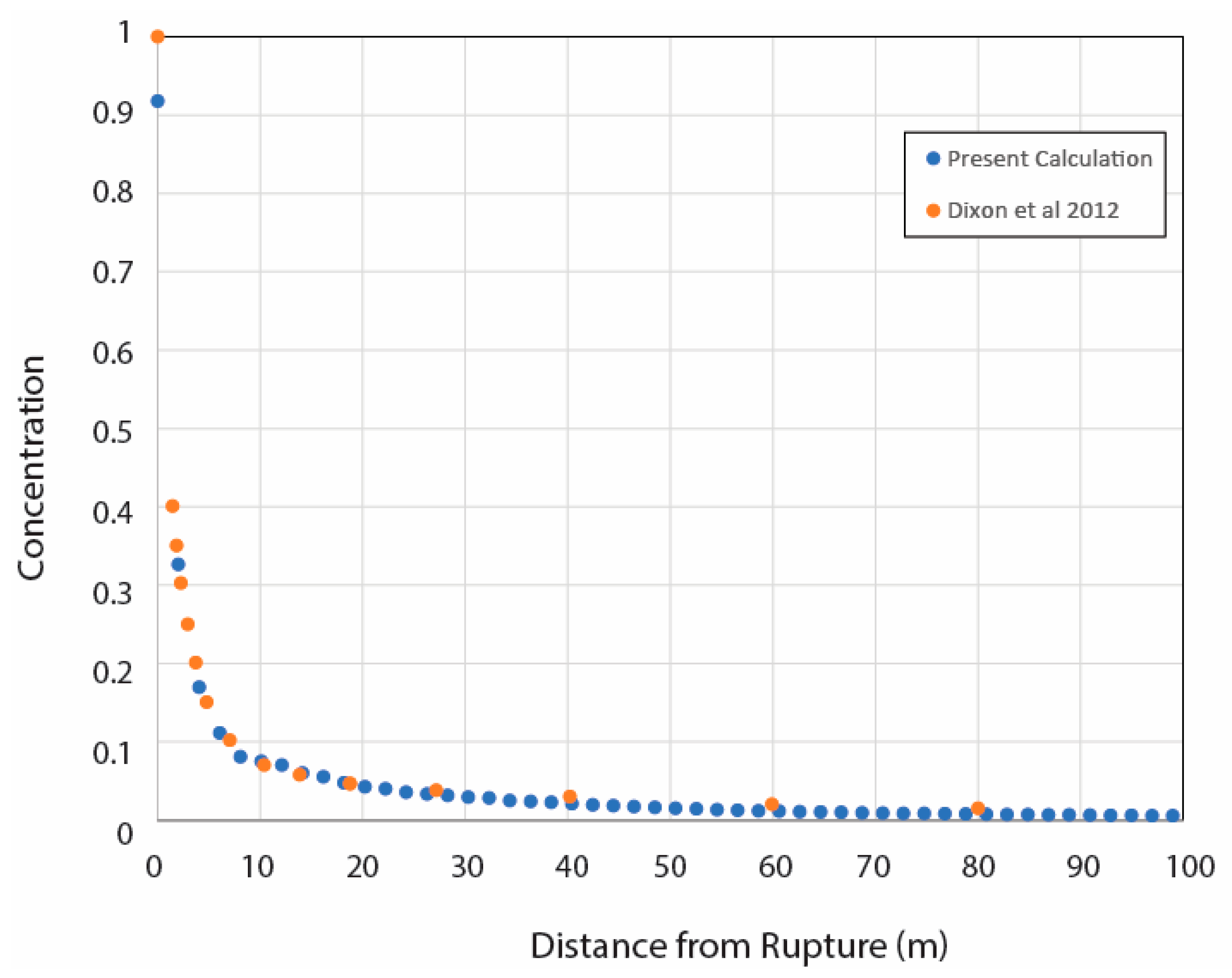
A second validation exercise was performed, this time by comparing the present calculations with [55]. In that study, carbon dioxide was released from a height of 1 m, and the release was oriented horizontally. Ref. [55] provided concentrations along the plume release direction; those values are provided in Figure 6. The corresponding results from the present simulation are also shown in the figure. As evident from the figure, there is excellent agreement between the experimental and simulation results.
With the present calculations providing excellent matches to two independent previously published studies, it increases confidence in the results and motivates continued use for other situations. It is noteworthy that for these CFD calculations, no calibrating parameters were employed to improve the validation. The calculations were carried out from first principles without modifying the model.

3.3. Real-World Model

Next, the simulations were expanded to a real-world, unintentional CO2 rupture. The rupture occurred near Satartia, MS, USA, on 22 February 2020. A 24-inch outer/23-inch inner diameter pipeline which had a pressure of 1336 psi ruptured and, as reported by the operator, released 31,000 barrels of CO2 (a portion of this volume was released intentionally after the initial rupture). The length between valves was 9.55 miles, and the rupture occurred 6.59 miles from the nearest upstream valve. The upstream valve was not closed until 10:25 p.m., more than three hours after the rupture (7:06 p.m.). The discharge of CO2 could have been higher than that used in this study, and, thus, the conclusions found here may be considered underestimates.
CO2 concentrations reportedly reached unsafe levels near the rupture and in Satartia, based on requests for medical assistance—to be discussed in more detail later. Figure 7 shows a topographic map of Satartia and the location of the rupture. The approximate distance from the rupture to the city is ~1.5 km. This topographical map was used to construct the computational topography. That is, the lines of elevation were inserted into the software. It is worthy to note that the present simulations generally applied a stair-step approach to topography; however, in the real world, terrain is smooth. The process of inputting topography levels into the software was burdensome and time consuming. Future efforts should be made to automate this process and to implement a smooth terrain rather than stair-stepping landscape.
Images of the pipeline after the rupture are provided in Figure 8. In the figure, solid CO2 is evident in white, and a crater has formed around the rupture site where the pressurized pipe was buried. The pressure within the pipeline was sufficient to remove significant amounts of soil (the crater’s depth was ~40 ft).
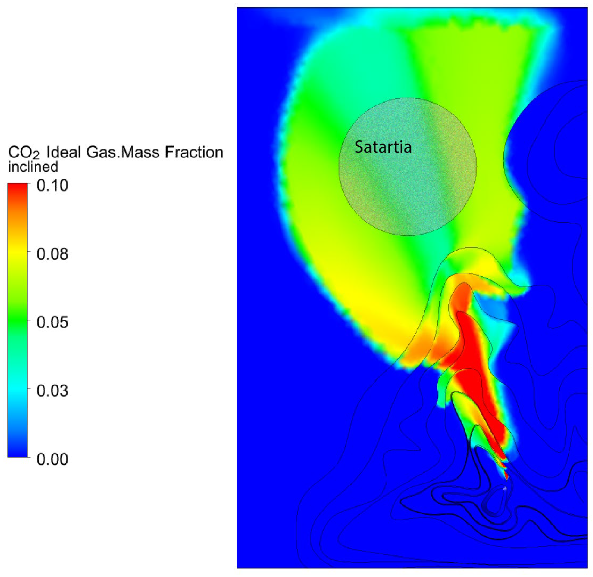
The rupture location was near a road at an elevated location. A geometric model of the typography is shown in Figure 9 with a top view (left) and an inclined view (right). The overall size of the solution domain is ~2000 m by 1250 m in the ground direction and 295 m in the vertical direction. At the time of failure, the operating pressure within the pipe was 1336 psi, and the pipe length was 77.4 miles. The solution domain extended far in the downstream direction because the prevailing wind carries the plume, and upwind dispersion is not expected.
At the left side of Figure 9, an inlet is provided with 5 miles/h (~2.2 m/s) wind, and the wind direction was from the E and SSE directions (taken from weather reports). While the wind speed and direction were constant in this study, it is routine to incorporate time-varying inlet conditions (velocity magnitude and direction) at the inlet location. In extreme cases, it is possible that the direction of wind would change to such a degree that what once was an inlet becomes an outlet and vice versa. This is no impediment for the software which can easily incorporate major changes in directions of wind flow (even 180-degree changes).
CO2 was in a gaseous phase at −70 °C and ambient pressure at the rupture. The very low temperature results from a high-pressure expansion and is consistent with experiments on released CO2 temperatures. After emerging from the rupture, the CO2 gas experienced temperatures changes as a consequence of mixing with ambient air. The densities of both species, CO2 and air, were allowed to vary based on local temperature and pressure. In real-world ruptures, a portion of the CO2 is transformed from gas to solid because of the rapid and significant temperature drop associated with the Joule–Thomson effect. Solid CO2 will subsequently sublimate to gas. The vast majority of the CO2 remains in the gaseous phase and previous studies have shown that solidification and fallout do not significantly affect the plume distance and size. Consequently, in this simulation, the entirety of CO2 was presumed to be gaseous at the rupture site.
The mass flow rate of CO2 exiting the rupture was estimated to be 250–500 kg/s. These estimates are based on the volume of material that was released, the duration of the release, and the pressure and temperature within the pipe, among others. The length between valves was 50,406 ft, which helps quantify the amount of CO2 that was released. While some researchers have applied discharge coefficients and the Bernoulli equation to estimate discharge rates, such calculations have high uncertainty for various reasons. First, the discharge coefficient is never known with high accuracy because the shape of the rupture hole is irregular, and the location of the rupture will affect the discharge coefficient. Second, the rate of discharge changes over time—beginning from an initial large value and decreasing over time as the pressure within the pipeline or vessel decreases. Because of these uncertainties, calculations will be carried out with multiple CO2 discharge rates. These rates are based on the density of the carbon dioxide within the pipeline prior to the rupture, the duration of the rupture, and the volume of carbon dioxide that was released. Among all the parameters, the discharge rate is one of the most important but the least certain, thus motivating calculations with different discharge values. Both of these discharge values are typical of ruptures from these types of pressurized vessels. When available, the real-time monitoring of pressure and temperature within pipelines can provide more accurate estimations of the discharge rate. Because of the great distances between the rupture and the nearby town of Satartia, the plume requires an extended period for travel, thereby allowing timewise average values to be used in the CFD calculations.
The ambient temperature was 15.5 °C (60 °F). At the ground–air interface, a no-slip boundary condition was applied—at the top, a free-slip boundary condition was used. At the solution domain’s downstream end, outlet conditions enforced a zero second derivative on all transported variables. The simulated CO2 injection was from a circular hole at the rupture location.
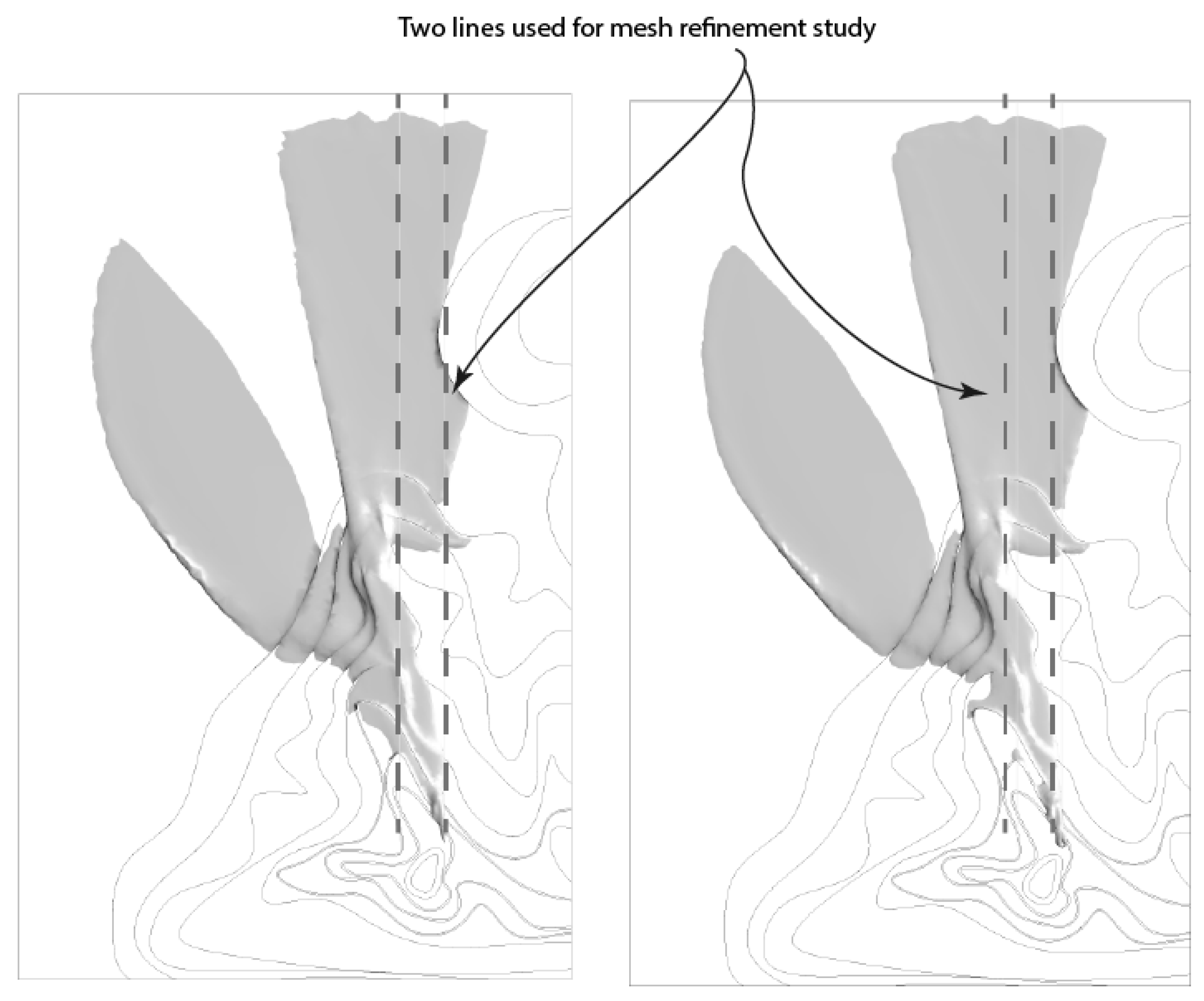
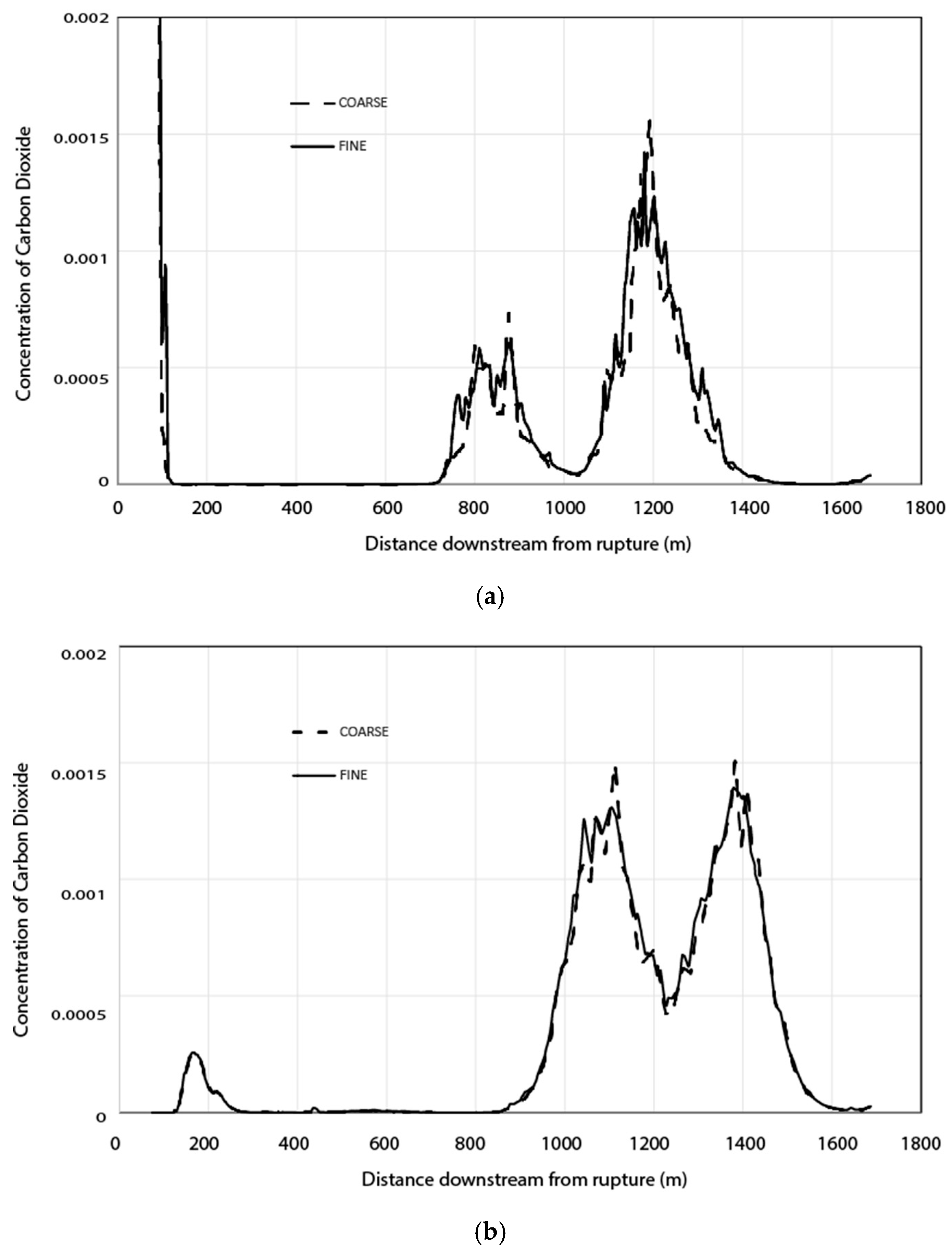
More refined geometry extraction may improve accuracy but also increase the time required to convert topographical maps to CFD models. It is important to ensure adequate elements are used to yield accurate calculations. To explore this, a mesh refinement study was performed. Multiple computational meshes were used to calculate concentration profiles as part of the mesh refinement. The size and location of the plumes for coarse and fine mesh simulations were compared. In addition, quantitative local information is used to demonstrate mesh independence because local values are more challenging to match. In Figure 10, there are two images, the left image corresponds to a coarse mesh and the right images is from the finer mesh. Two lines indicate where the concentrations will be obtained. One dashed line passes through the rupture orifice, while a second line is 100 m west (to the left in the figure) of the rupture location and at a 61 m elevation compared Satartia. Carbon dioxide concentrations will be obtained at 1000 sampling points along these two dashed lines.
These results are in excellent agreement (both the plume size/location and local concentration values). A similar conclusion would have resulted if other locations had been used in the mesh independence study. In Figure 11a, the concentrations are initially very high because the line passes through the rupture orifice. For both sampling lines, there are downstream local maxima of concentration, and both the coarse and fine mesh agree very well on the locations and magnitudes of the maxima.
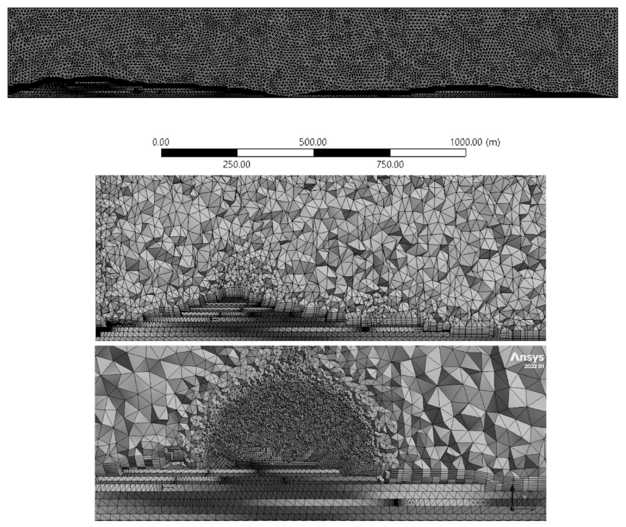
Figure 12 shows three images of the final computational mesh used in the real-world calculation. The geometry was obtained from the already discussed topographical maps, and elevation levels were incorporated into the model. The uppermost image and a scale below the figure show the entire solution domain. The second and third figures show elements that follow the topology. From all images, particularly from the second image, boundary layer elements can be seen deployed along the air–ground interface. These elements are used to capture the velocity gradients in the boundary layer. The third image shows refined elements near the rupture—these smaller elements more accurately capture the emerging jet. The final number of elements was 36 million. The elements generally ranged in size from 1 m to 20 m; however, in the near vicinity of the rupture, elements were 10 cm. The y+ value between the flow and ground ranged from 18–350. These y+ values required the use of scalable logarithmic wall functions. This approach has a strong record of allowing integration from the freestream to a no-slip boundary.
Table 3 is provided with respect to the parameters that govern the calculation. The boundary conditions and the mathematical model have already been discussed. Insofar as the initial jet velocity can be very high, the analysis included compressibility effects. It was found that the final results were very similar regardless of whether compressible effects were accounted for.
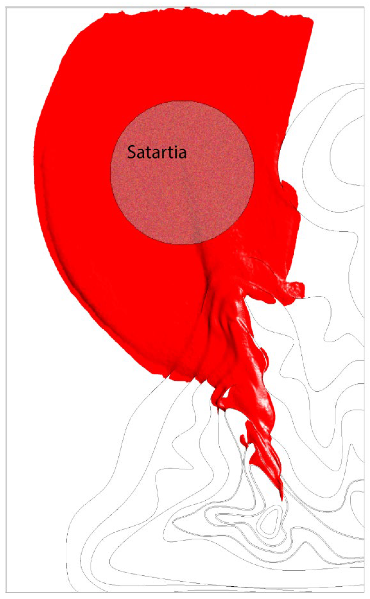
Upon completion of the calculations, the downstream concentration of CO2 was found. Figure 13 shows the region impacted by 5% CO2 concentrations. At this point, it is noteworthy that the calculations were time averaged. The calculations were not designed to quantify small-scale concentration variations due to transient air motion. Performing a transient calculation is possible but is time-consuming and less practical. A consequence of this fact means that areas within the 5% time-averaged concentration plume will experience transient concentrations both above and below 5%. Conservatively, it is expected that within the red zone, concentrations could be as low as ~0% and as high as ~10%. At the same time, locations not within the red plume regions can experience concentrations up to and exceeding 5% for short durations—even though the time-averaged values of CO2 concentration are less than 5%. Concentrations of 5% were chosen for display in Figure 13 because of their proximity to toxic levels of CO2. The total ground area covered by a plume in excess of 5% CO2 is 630,000 m2.
As evident in Figure 13, there is a bifurcation in high CO2 concentrations that is caused by topographical features. Portions of the east and western parts of Satartia experienced higher CO2 concentrations than the center of the town. However, all parts of the town experienced potentially dangerous carbon dioxide levels.
In Figure 14, a continuous distribution of ground-level CO2 is shown from a top-down perspective. It is seen there that the plume decreases in concentration (from 10% near the rupture to ~5% at Satartia). As the plume spreads, the concentrations decrease. At the top of the image, the plume concentrations have decayed to less than 5%.
The calculation results set forth in Figure 13 and Figure 14 correspond to a CO2 mass flowrate of 500 kg/s. Notably, the plume traveled from the rupture site to Satartia in approximately 8 min—a very short time compared to the multi-hour duration of the rupture. Since the actual flow rate is not known with certainty and depends upon factors such as the size of the rupture, the pressure and temperature within the tube, the diameter of the tube, and the distance between valves, a sensitivity analysis is appropriate. To explore the impact of mass flow rate on the downstream plume, calculations were repeated with ~250 kg/s. Figure 15 shows the corresponding results. The red-colored plume represents a 3% concentration. As shown in the figure, the nearby town of Satartia was completely engulfed by the 3% concentration. It should be recalled that these calculations are timewise averages. It can reasonably be expected that in a real-world situation, with variable wind speeds and small-scale eddies, the actual concentration in the plume region could be as low as 0% or as high as ~6%. The total surface area covered by a 3% time-averaged concentration is 1 million square meters. The results from Figure 13, Figure 14 and Figure 15 are consistent with Satartia residents seeking medical treatment following the unintentional rupture. Notably, as part of this study, the ALOHA dispersion model was employed to predict the extent of the Satartia plume—it greatly underpredicted the distance the plume traveled. Similarly, the PHAST model was also found to underpredict the plume distance.
Some commentary about model accuracy is relevant. This paper documents excellent agreement between the numerical model and two separate validation studies. The two validation studies use the same computational approach, the same turbulence modeling equations, the same conservation of mass, momentum, and energy equations, similar buoyancy treatment, and boundary conditions. The main missing ingredient in the validation studies is the varying topography. With body-fitted computational elements, there is no impediment to the ability of software to handle topography. In fact, varying topography is routinely encountered in simulation studies. Based on this observation, we consider the validation studies to be useful indicators of the ability of CFD to predict plumes.
Following the validation exercise, the model was applied to a real-world scenario for which validation data are not available. In fact, to the best knowledge of the authors, there have not been concentration measurements at the time of an unintended rupture such as that which occurred near the town of Satartia. Measurements of unintentional ruptures is difficult because they are, by definition, unintentional, and they occur at times and places that are unexpected.
In view of the above discussion, we are not making claims of the absolute accuracy of the real-world calculations. However, we do assert that the output of the real-world CFD matches records of persons seeking medical attention. We also assert that that CFD can be used as a tool to assess safety. In fact, as noted earlier, results from CFD modeling indicate a risk for inhabitants of Satartia, whereas dispersion modeling of the same rupture failed to identify any risk. Thus, we claim that in the real-world, CFD can help identify locations where an unintentional rupture may present a health risk. We also claim that CFD models can complement more crude dispersion calculations—particularly in varying terrain areas, situations with changing weather conditions, and situations where a pipeline passes close to an inhabited region.

3.4. Selection of CFD and Dispersion Models

With the results presented so far, it is clear that CFD models provide certain advantages over simplified dispersion models. In particular, CFD can handle non-flat terrain, obstacles, timewise or spatial variations in wind and ambient conditions, variations to the direction of release, etc. On the other hand, CFD models generally require more time and effort to construct and, therefore, may not be viable for real-time information following a rupture. The advantages of CFD models persist in a pipeline’s planning and routing stages.
To further elucidate this issue, Figure 16 is presented. This image lists the fraction of time for which the predictions from dispersion models are within a factor of two with the observations. It can be recognized that all of these dispersion models have great difficulty in matching actual plume concentrations—within a factor of two is a poor performance threshold and indicates a clear limitation of the simplified dispersion models. In real-world applications, predictions within a factor of two would give very little assurance to persons in the plume-affected area.
Further concerns about dispersion models are apparent when dispersion predictions are compared. In Figure 17, such a comparison is provided. This comparison utilized chlorine, but the discrepancy of dispersion models is seen regardless of the rupture medium. As apparent in the figure, at a distance of 100 m, there is a factor of ~20 difference between the predictions. At a distance of 1 km, the spread amongst the models is ~350%. At a distance of 10 km from the rupture, the spread amongst the models is ~300%. Clearly, the large spread amongst dispersion models is a concern regarding the use of dispersion models for plume predictions.
Based on these results (the present CFD calculations and past dispersion model results, it is apparent that the improved accuracy of CFD over dispersion models justifies their continued exploration.

4. Concluding Remarks

This study has focused on applying computational fluid dynamics (CFD) for plume modeling. In particular, validation test cases were performed to demonstrate the viability of CFD for making accurate predictions. In addition, a real-world calculation of a ruptured CO2 pipeline was performed, and the CFD predictions indicate that a nearby town would be at risk. These results are supported by several people in the town who sought medical attention following the rupture. Based on these results and on the previously available literature, CFD is found to be a valuable method for determining the downstream concentrations from a rupture.
The alternative approach of a simplified dispersion model was also discussed. While dispersion models are simpler to use and provide results more rapidly, their accuracy is a concern. Dispersion models did not accurately predict the risk that a rupture would present to the town of Satartia. In addition, dispersion models are limited in their inability to handle non-flat terrain, obstacles, and variations in wind speed and other environmental conditions. In fact, dispersion models are built upon assumed concentration profiles that are unlikely to occur in the real world.
While CFD models can make more accurate predictions, they should not supplant simplified dispersion models. Their ease of use and rapid results ensure that dispersion models can continue to play an important role—particularly after a rupture. However, CFD should be utilized in planning and routing stages when pipelines pass near high-consequence areas or where ruptures are more likely.
Among the practical challenges that are faced with in these types of CFD calculations is the accurate modeling of topography—topographical information must be integrated with the CAD model, and currently, this is a manual practice. Future efforts should be undertaken to automatize this. Other inputs, however, are relatively easy to implement. For example, weather conditions are generally available in many developing world countries.
The results of this study demonstrate that CFD can play an important role in improving the safety of pressurized pipelines. First, CFD can be performed during the routing of a pipeline at critical locations where pipelines are close to high-consequence zones. The completion of such calculations will help improve routing to maintain safe distances between the pipeline and inhabited regions. In addition, CFD results at critical locations along a pipeline can be relied upon if a rupture were to occur—plume trajectories calculated for a variety of weather/wind conditions would be made available because of the simulations. These calculations would let first responders know, at the time of a rupture, whether the prevailing weather conditions would bring a plume to a high-risk location. The use of CFD is meant to complement faster and more crude dispersion modeling. Those modeling studies could, conceivably, be performed when a rupture occurs to provide near real-time plume information to first responders. It should be noted, however, that real-time calculations with dispersion models may potentially underpredict the risk to inhabitants. Both methods, used complementarily, are a state-of-the-art standard for pipeline safety.
The present calculations relate to a post facto study of a rupture. We are not suggesting that CFD’s main role is after a rupture occurs—by that time, the risk has already occurred. The real role of CFD is to be completed before a rupture—during planning, routing, and risk assessment. The reason the present calculations were post facto is that only in retrospect is there a real-world eruption that can be used to demonstrate the suitability of CFD for these types of calculations.

Author Contributions

Methodology, J.A. and J.G.; Software, J.G.; Validation, J.A. and L.C.; Formal analysis, L.C.; Investigation, J.A.; Writing—review & editing, L.C. and J.G. All authors have read and agreed to the published version of the manuscript.

Funding

This research received no external funding.

Data Availability Statement

Data are contained within the article.

Conflicts of Interest

Author J.P. Abraham has testified, pro bono, at a hearing involving the safety of CO2 pipeline ruptures. The remaining authors declare that the research was conducted in the absence of any commercial or financial relationships that could be construed as a potential conflict of interest.

References

  1. Abraham, J.P.; Cheng, L.; Mann, M.E.; Trenberth, K.E.; von Schuckmann, K. The Ocean Response to Climate Change Guides Both Adaptation and Mitigation Efforts. Atmos. Ocean. Sci. Lett. 2022, 15, 100221. [Google Scholar] [CrossRef]
  2. Cheng, L.; Foster, G.; Hausfather, Z.; Trenberth, K.E.; Abraham, J.P. Improved Quantification of the Rate of Ocean Warming. J. Clim. 2022, 35, 4827–4840. [Google Scholar] [CrossRef]
  3. Cheng, L.; Abraham, J.; Trenberth, K.E.; Fasullo, J.; Boyer, T.; Mann, M.E.; Zhu, J.; Wang, F.; Locarnini, R.; Li, Y.; et al. Another Year of Record Heat for the Oceans. Adv. Atmos. Sci. 2023, 40, 963–974. [Google Scholar] [CrossRef] [PubMed]
  4. Cheng, L.; Abraham, J.; Trenberth, K.E.; Boyer, T.; Mann, M.E.; Zhu, J.; Wang, F.; Yu, F.; Locarnini, R.; Fasullo, J.; et al. New Record Ocean Temperatures and Related Climate Indicators in 2023. Adv. Atmos. Sci. 2024, in press. [Google Scholar] [CrossRef]
  5. Mazzoldi, A.; Hill, T.; Colls, J.J. A Consideration of the Jet-Mixing Effect when Modeling CO2 Emissions from High-Pressure CO2 Transportation Facilities. Energy Procedia 2009, 42, 1571–1578. [Google Scholar] [CrossRef]
  6. Permentier, K.; Vercammen, S.; Soetaert, S.; Schellemans, C. Carbon Dioxide Poisoning: A Literature Review of an Often Forgotten Cause of Intoxication in the Emergency Department. Int. J. Emerg. Med. 2017, 10, 14. [Google Scholar] [CrossRef] [PubMed]
  7. Department of Health and Human Services; National Institute for Occupational Safe. NIOSH Pocket Guide to Chemical Hazards; DHSS (NIOSH) Publication no. 2005-149; Scholar’s Choice: London, UK, 2015. [Google Scholar]
  8. Woodward, J.L.; Cook, J.; Papadourakis, A. Modeling and Validation of a Dispersing Aerosol Jet. J. Hazard. Mater. 1995, 44, 185–207. [Google Scholar] [CrossRef]
  9. Woodward, J.L.; Papadourakis, A. Reassessment and reevaluation of rainout and drop zie correlation for an aerosol jet. J. Hazard. Mater. 1995, 44, 209–230. [Google Scholar] [CrossRef]
  10. Ermak, D. Users Manual for Slab: An Atmospheric Dispersion Model for Denser-than-Air Releases; Lawrence Livermore Laboratory: Livermore, CA, USA, June 1990. [Google Scholar]
  11. Colenbrander, G.W. A mathematical model for the transient behaviour of dense vapor clouds. In Proceedings of the 3rd International Symposium on Loss Prevention and Safety Promotion in the Process Industries, Basel, Switzerland, 15–18 September 1980. [Google Scholar]
  12. Havens, J. A Dispersion Model for Elevated Dense Gas Jet Chemical Releases, Vol. II: Users Guide; U.S. Environmental Protection Agency: Durham, NC, USA, 1988.
  13. Liu, X.; Godbole, A.; Lu, C.; Michal, G.; Venton, P. Optimization of Dispersion Parameters of Gaussian Plume Model for CO2 Dispersion. Environ. Sci. Pollut. Res 2015, 22, 18288–18299. [Google Scholar] [CrossRef]
  14. Witlox, H.; Holt, A. A Unified Model for Jet, Heavy, and Passive Dispersion Including Droplet Rainout and Re-evaporation. Center for Chemical Process Safety Conference. 1999. Available online: https://www.researchgate.net/profile/Henk-Witlox/publication/265566709_A_unified_model_for_jet_heavy_and_passive_dispersion_including_droplet_rainout_and_re-evaporation/links/54bcf5b50cf253b50e2d8830/A-unified-model-for-jet-heavy-and-passive-dispersion-including-droplet-rainout-and-re-evaporation.pdf (accessed on 1 February 2024).
  15. Witlox, H.; Harper, M.; Oke, A. Modeling of Discharge and Atmospheric Dispersion for Carbon Dioxide Release. J. Loss Prev. Process Ind. 2009, 22, 795–802. [Google Scholar] [CrossRef]
  16. Witlox, H.; Harper, M.; Oke, A. PHAST Validation of Discharge and Atmospheric Dispersion for Pressurized Carbon Dioxide Releases. In Proceedings of the Hazards XXIII Symposium Series 158, Southport, UK, 12–15 November 2012. [Google Scholar]
  17. Hill, T.A.; Fackrell, J.E.; Dubal, M.R.; Stiff, S.M. Understanding the Consequences of CO2 Leakage Downstream of the Capture Plant. Energy Procedia 2011, 4, 2230–2237. [Google Scholar] [CrossRef]
  18. Gant, S.E.; Kelsey, A.; McNally, K.; Witlox, H.; Bilio, M. Sensitivity Analysis of Dispersion Models for Jet Releases of Dense-Phase Carbon Dioxide. Chem. Eng. Trans. 2013, 31, 121–125. [Google Scholar]
  19. Gant, S.E.; Narasimhamurthy, V.D.; Skjold, T.; Jamois, D.; Proust, C. Evaluation of multi-Phase Atmospheric Dispersion Models for Application to Carbon Capture and Storage. J Loss Prev. Process Ind. 2014, 32, 286–298. [Google Scholar] [CrossRef]
  20. Liu, X.; Godbole, A.R.; Lu, C.; Michal, G. Investigation of Terrain Effects on the Consequence Distance of CO2 Released from High-Pressure Pipelines. Fac. Eng. Inf. Sci.–Pap. Part B 2017, 66, 995. [Google Scholar]
  21. Liu, X.; Godbole, A.; Lu, C.; Guillaume, M.; Linton, V. Consequence Modeling of CO2 Pipeline Failure. Energy Procedia. 2019, 159, 5109–5115. [Google Scholar] [CrossRef]
  22. Pontiggia, M.; Derudi, M.; Nusini, V.; Rota, R. Hazardous Gas Dispersion: A CFD model Accounting for Atmospheric Stability Classes. J. Hazard. Mater. 2009, 171, 739–747. [Google Scholar] [CrossRef] [PubMed]
  23. Hsieh, K.J.; Lien, F.S.; Tee, E. Dense Gas Dispersion Modeling of CO2 Released from Carbon Capture and Storage Infrastructure into a Complex Environment. Int. J. Greenh. Gas Control 2013, 17, 127–139. [Google Scholar] [CrossRef]
  24. Wen, J.; Heidari, A.; Xu, B.; Jie, H. Dispersion of Carbon Dioxide from Vertical Vent and Horizontal Releases—A Numerical Study. Proc. Inst. Mech. Eng. Part E J. Process Mech. Eng. 2013, 227, 125–139. [Google Scholar] [CrossRef]
  25. Xing, J.; Liu, Z.; Huang, P.; Zhou, Y.; Zhang, D.; Wang, F. Experimental and numerical study of the dispersion of carbon dioxide plume. J. Hazard. Mater. 2013, 256–257, 40–48. [Google Scholar] [CrossRef]
  26. Sklavounos, S.; Rigas, F. Validation of Turbulence Models in Heavy Gas Dispersion over Obstacles. J. Hazard. Mater. 2004, 108, 9–20. [Google Scholar] [CrossRef]
  27. Wang, H.; Zhanpang, Y.; Fan, M.; Bin, L.; Peng, H. Study on Dispersion of Carbon Dioxide over the Shrubbery Region. Front. Energy Res. 2021, 9, 695224. [Google Scholar]
  28. Wang, H.; Liu, B.; Liu, X.; Deng, J.; You, Z. Dispersion of Carbon Dioxide Released from Buried High-Pressure Pipeline Over Complex Terrain. Environ. Sci. Pollut. Res. Int. 2021, 28, 6635–6648. [Google Scholar] [CrossRef] [PubMed]
  29. Woolley, R.M.; Fairweather, M.; Wareing, C.J.; Falle, S.A.; Mahgerefteh, H.; Martynov, S.; Brown, S.; Narasimhamurthy, V.D.; Storvik, I.E.; Sælen, L.; et al. CO2PipeHaz: Quantitative Hazard Assessment for Next Generation CO2 Pipelines. In Proceedings of the 12th International Conference on Greenhouse Gas Technologies (GHGT-12), Austin, TX, USA, 5 October 2014. [Google Scholar]
  30. Godbole, A.; Liu, X.; Michael, G.; Davis, M.; Lu, C.; Armstrong, K.; Medina, C.H. Atmospheric Dispersion of CO2 Following Full-Scale Burst Tests. In Proceedings of the 14th International Convection on Greenhouse Gas Control Technologies (GHGT-14), Melbourne, Australia, 21–25 October 2018. [Google Scholar]
  31. Peterson, R.L. Effect of Homogeneous and Heterogeneous Surface Roughness on Heavier-than-Air-Gas Dispersion. J. Wind Eng. Ind. Aerodyn. 1990, 36, 643–652. [Google Scholar] [CrossRef]
  32. Hanna, S.R.; Chang, J.C. Use of the Kit Fox data to analyze dense gas dispersion modeling issues. Atmos. Environ. 2001, 35, 2231–2242. [Google Scholar] [CrossRef]
  33. Mack, A.; Spruijt, M.P.N. CFD Dispersion Investigation of CO2 Worst Case Scenarios Including Terrain and Release Effects. Energy Procedia 2014, 51, 363–372. [Google Scholar] [CrossRef]
  34. Mazzoldi, A.; Hill, T.; Colls, J. CFD and Gaussian Atmospheric dispersion models: A comparison for leak from Carbon Dioxide Transportation and Storage Facilities. Atmos. Environ. 2008, 42, 8046–8054. [Google Scholar] [CrossRef]
  35. Ahmad, M.; Lowesmith, B.; De Koeijer, G.; Nilsen, S.; Tonda, H.; Spinelli, C.; Cooper, R.; Clausen, S.; Mendes, R.; Florisson, O. COSHER Joint Industry Project: Large Scale Pipeline Rupture Tests to Study CO2 Release and Dispersion. Int. J. Greenh. Gas Control 2015, 37, 340–353. [Google Scholar] [CrossRef]
  36. Yan, X.; Guo, X.; Yu, J.; Chen, S.; Zhang, Y.; Mahgerefteh, H.; Martynov, S.; Brown, S. Flow and Characteristics and Dispersion Du ring the Vertical Anthropogenic Venting of Supercritical CO2 from an Industrial Scale Pipeline. Energy Procedia 2018, 154, 66–72. [Google Scholar] [CrossRef]
  37. Zhou, X.; Li, K.; Tu, R.; Xie, Q.; Jiang, X. A Modelling Study of the Multiphase Leakage Flow from Pressurized CO2 Pipeline. J. Hazard. Mater. 2016, 305, 286–294. [Google Scholar] [CrossRef]
  38. Vitali, M.; Zuliani, C.; Corvaro, F.; Marchetti, B.; Terenzi, A.; Tallone, F. Risks and Safety of CO2 Transport via Pipeline: A Review of Risk Analysis and Modeling Approaches for Accidental Releases. Energies 2021, 14, 4601. [Google Scholar] [CrossRef]
  39. Hanna, S.R.; Steinberg, K.W. Overview of Petroleum Environmental Research Forum (PERF) Dense Gas Dispersion Modeling. Atmos. Environ. 2001, 35, 2223–2229. [Google Scholar] [CrossRef]
  40. Hanna, S.R.; Strimaitis, D.G.; Chang, J.C. Hazard Response Modeling Uncertainty (A Quantitative Method) Vol. II—Evaluation of Commonly Used Hazardous Gas Dispersion Models; Report No. ESL-TR-01-29; Sigma Research Corporation: Westford, MA, USA, 1993. [Google Scholar]
  41. Pouyakian, M.; Ashouri, M.; Eidani, S.; Madvari, R.F.; Laal, F. A systematic review of Consequence Modeling Studies of the Process Accidents in Iran from 2006 to 2022. Heliyon 2023, 9, e13550. [Google Scholar] [CrossRef] [PubMed]
  42. Alivi, A.T.; Shahraki, F.; Sardashti Birjandi, M.R.; Khalilipour Langerudi, M.M. Consequence Moedling and Determining of Safe Distance in the Natural Gas Pressure Reduction Station Using PHAST Software (Case Study Borumi Station in Ahvax). Occup. Med. 2023, 15, 37–57. [Google Scholar]
  43. Ghasemi, M.; Givehchi, S.; Nasrabadi, M. Modeling the Outcome of Tank Explosion Using PHAST Software and Presentations of Emergency Operations Plan (Case Study: Ethylene Tank of Kavian Petrochemical Company). J. Fundam. Appl. Sci. 2016, 8, 2007–2021. [Google Scholar]
  44. Wang, B.; Chen, B.; Zhao, J. The Real-Time Estimation of Hazardous Gas Dispersion by the Integration of Gas Detectors, Neural Network and Gas Dispersion Models. J. Hazard. Mater. 2015, 300, 433–442. [Google Scholar] [CrossRef] [PubMed]
  45. Dai, Y.; Mak, C.M.; Ai, Z.; Hang, J. Evaluation of Computational and Physical Parameters Influencing CFD Simulations of Pollutant Dispersion in Building Arrays. Build. Environ. 2018, 137, 90–107. [Google Scholar] [CrossRef]
  46. Ai, Z.T.; Mak, C.M. Large-Eddy Simulation of Flow and Dispersion Around an Isolated Building: Analysis of Influencing Factors. Comput. Fluids 2015, 118, 89–100. [Google Scholar] [CrossRef]
  47. Abraham, J.P.; Plourde, B.D.; Vallez, L.J. Comprehensive Review and Study of Buoyant Air Flow Within Positive-Pressure Hospital Operating Rooms. Numer. Heat Transf. A 2018, 72, 1–20. [Google Scholar] [CrossRef]
  48. ANSYS. ANSYS-CFX Solver Theory; ANSYS, Inc.: Canonsburg, PA, USA, 2023. [Google Scholar]
  49. Sparrow, E.M.; Abraham, J.P. A New Buoyancy Model Replacing the Standard Pseudo-Density Difference for Internal Natural Convection in Gases. Int. J. Heat Mass Transf. 2003, 46, 3583–3591. [Google Scholar] [CrossRef]
  50. Minkowycz, W.J.; Abraham, J.P.; Sparrow, E.M. Numerical Simulation of Laminar Breakdown and Subsequent Intermittent and Turbulent Flow in Parallel Plate Channels: Effects of Inlet Velocity Profile and Turbulence Intensity. Int. J. Heat Mass Transf. 2009, 52, 4040–4046. [Google Scholar] [CrossRef]
  51. Olsen, L.E.; Abraham, J.P.; Cheng, L.J.; Gorman, J.M.; Sparrow, E.M. Summary of Forced-Convection Fluid Flow and Heat Transfer for Square Cylinders of Different Aspect Ratios Ranging from the Cube to a Two-Dimensional Cylinder. Adv. Heat Transf. 2019, 51, 351–457. [Google Scholar]
  52. Abraham, J.P.; Bhattacharya, S.; Cheng, L.; Gorman, J.M. A Brief History of and Introduction to Computational Fluid Dynamics. In Computational Fluid Dynamics; Bhattacharya, S., Ed.; IntechOpen: London, UK, 2021. [Google Scholar]
  53. Gorman, J.; Bhattacharya, S.; Abraham, J.P.; Cheng, L. Turbulence Models Commonly used in CFD. In Computational Fluid Dynamics; Bhattacharya, S., Ed.; IntechOpen: London, UK, 2021. [Google Scholar]
  54. Menter, F. Two-Equation Eddy-Viscosity Turbulence Models for Engineering Applications. AIAA J. 1994, 32, 1598–1605. [Google Scholar] [CrossRef]
  55. Dixon, C.M.; Gant, S.E.; Obiorah, C.; Bilio, M. Validation of Dispersion Models for High Pressure Carbon Dioxide Releases. In Proceedings of the Hazards XXIII Symposium Series, Southport, UK, 12–15 November 2012; pp. 153–163. [Google Scholar]
  56. Liu, Y.; Ozbayoglu, E.M.; Upchurch, E.R.; Baldino, S. Computational Fluid Dynamics Simulations of Taylor Bubbles Rising in Vertical and Inclined Concentric Annuli. Int. J. Multiph. Flow 2023, 159, 104333. [Google Scholar] [CrossRef]
  57. Liu, Y.; Mitchell, T.; Upchurch, E.R.; Ozbayoglu, E.M.; Baldino, S. Investigation of Taylor Bubble Dynamics in Annula Conduits with Counter-Current Clow. Int. J. Multiph. Flow 2024, 170, 104626. [Google Scholar] [CrossRef]
  58. Ke, W.; Zeng, H.; Wang, Z.; Yu, H.; Liu, Y.; Zheng, D.; Zhu Jianjun, Z.; Zhu, H. A Numerical Study on Labyrinth Screw Pump (LSP) Performance Under Viscous Fluid Flow. Energies 2023, 16, 5997. [Google Scholar] [CrossRef]
  59. Brown Coal Innovation Australia Limited. Dispersion Modelling Techniques for Carbon Dioxide Pipelines in Australia; Document no. 20873-RP-001; Brown Coal Innovation Australia Limited: Melbourne, Australia, 2015; pp. 1–193.
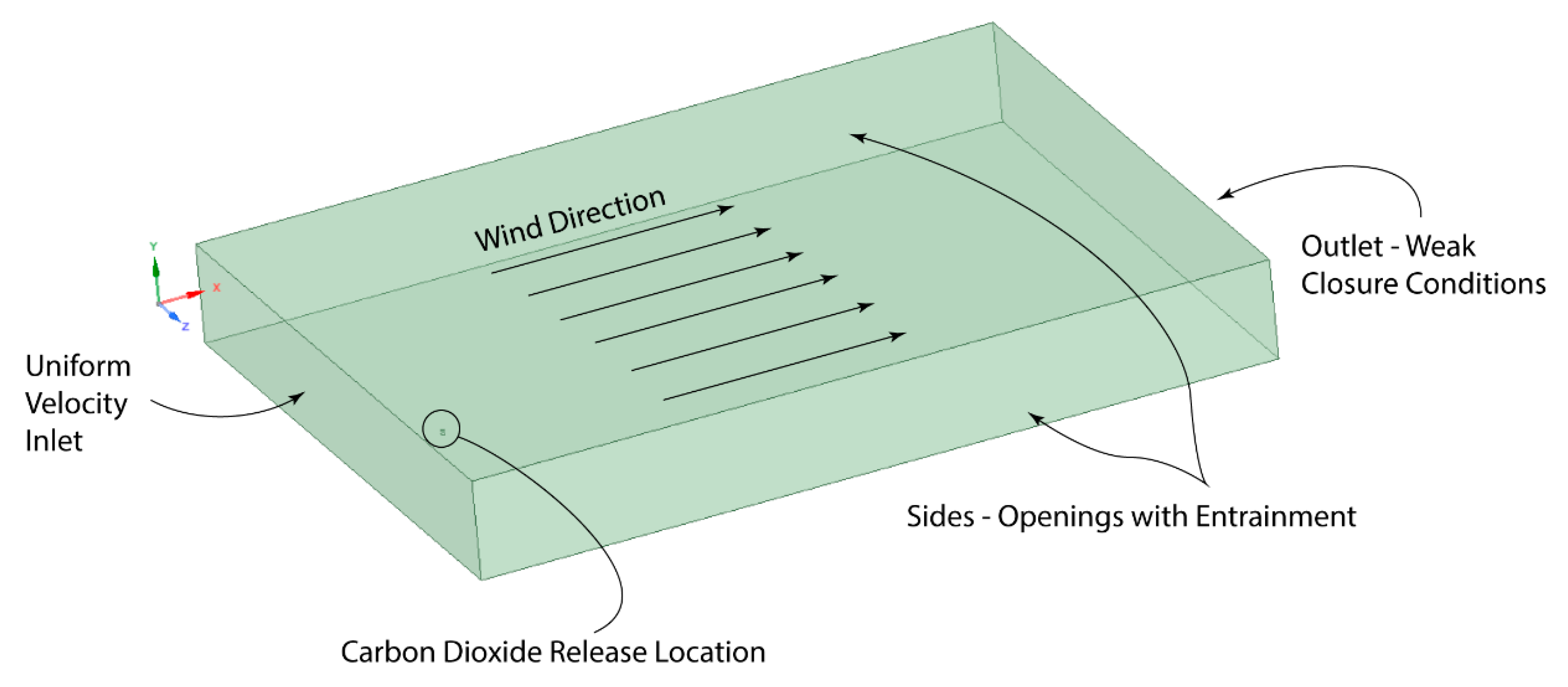
Figure 1. Computational domain for validation test cases.
Energies 17 01079 g001
Figure 2. The computational mesh for validation studies.
Energies 17 01079 g002
Figure 3. CO2 concentrations for validation calculation 9 just downstream of the rupture location.
Energies 17 01079 g003
Figure 4. Iso-concentration area for 10% CO2 concentration.
Energies 17 01079 g004
Figure 5. Iso-concentration area for 2% CO2 concentration.
Energies 17 01079 g005
Figure 6. Comparison of the present calculations with results from Dixon et al., 2012 [55].
Energies 17 01079 g006
Figure 7. Topographical map near Satartia.
Energies 17 01079 g007
Figure 8. (a) Photograph of the ruptured pipeline from above; (b) closeup photograph of the ruptured pipeline.
Energies 17 01079 g008
Figure 9. Top and inclined views of the geometric model extracted from the topography map.
Energies 17 01079 g009
Figure 10. Comparison of plume size and position (grey region) and the identification of two sampling lines used for a more rigorous comparison. The left image corresponds to a coarse mesh whereas the right image corresponds to a fine mesh. with the plume has a 500 kg/s rupture release rate.
Energies 17 01079 g010
Figure 11. Comparisons of concentration values along two testing lines: (a) a line passing northwards and passing through the center of the rupture; (b) a parallel line positioned 100 m to the west, both lines at a 61 m elevation with respect to Satartia. The coarse mesh has ~3 million elements, and the fine mesh has ~36 million elements. Plume with 500 kg/s.
Energies 17 01079 g011
Figure 12. Computational mesh for Satartia plume calculations.
Energies 17 01079 g012
Figure 13. View from above—calculated 5% plume extent (500 kg/s discharge).
Energies 17 01079 g013
Figure 14. View from above—ground-level CO2 concentration contour (500 kg/s discharge).
Energies 17 01079 g014
Figure 15. View from above—calculated 3% plume extent with 250 kg/s CO2 flow.
Energies 17 01079 g015
Figure 16. Graphic showing the reported performance of various dispersion models [40].
Energies 17 01079 g016
Figure 17. Comparison of dispersion model results indicating a lack of agreement from [59].
Energies 17 01079 g017
Table 1. Settings for two validation calculations.
ParameterTest 9Test 11
Storage pressure (atm)15281
Ambient temperature (°C)8.211.6
Ambient pressure (atm)0.950.95
Wind speed (m/s)4.045.99
Discharge rate (kg/s)6.057.12
Discharge temperature (°C)−70−70
Orifice diameter (mm)11.9411.94
Orifice opening area (mm2)112112
Table 2. Comparison of numerical simulations to experimental observations for two test cases, measurements made 40 m downwind of release [16].
Case No.Experimental (%)CFD (%)PHAST (%)
91.92.11.3
113.42.31.9
Table 3. Settings for in-field calculations.
ParameterInputs
Pipe OD and ID (inches)24 and 23
Pipeline pressure (psi)1336
Ambient temperature (°C, °F)15.5 °C, 60 °F
Wind speed (m/s)2.25
Discharge rates (kg/s)250 and 500
Discharge temperature (°C, °F)−56 °C, −70 °F
CO2 released (barrels)31,000
Disclaimer/Publisher’s Note: The statements, opinions and data contained in all publications are solely those of the individual author(s) and contributor(s) and not of MDPI and/or the editor(s). MDPI and/or the editor(s) disclaim responsibility for any injury to people or property resulting from any ideas, methods, instructions or products referred to in the content.