A Data-Driven Prediction Method for Proton Exchange Membrane Fuel Cell Degradation

Abstract

This paper proposes a long short-term memory (LSTM) network to predict the power degradation of proton exchange membrane fuel cells (PEMFCs), and in order to promote the performance of the LSTM network, the ant colony algorithm (ACO) is introduced to optimize the hyperparameters of the LSTM network. First, the degradation mechanism of PEMFCs is analyzed. Second, the ACO algorithm is used to set the learning rate and dropout probability of the LSTM network combined with partial aging data, which can show the characteristics of the dataset. After that, the aging prediction model is built by using the LSTM and ACO (ACO-LSTM) method. Moreover, the convergence of the method is verified with previous studies. Finally, the fuel cell aging data provided by the Xiangyang Da’an Automotive Testing Center are used for verification. The results show that, compared with the traditional LSTM network, ACO-LSTM can predict the aging process of PEMFCs more accurately, and its prediction accuracy is improved by about 35%, especially when the training data are less. At the same time, the performance of the model trained by ACO-LSTM is also excellent under other operating conditions of the same fuel cell, and it has strong versatility.

1. Introduction

Since the 21st century, countries around the world have seen a growing demand for efficient and low-emission new energy. Hydrogen energy, as a type of new energy, has been defined as the “ultimate energy source” and has garnered widespread attention in recent years. PEMFCs, as devices capable of efficiently utilizing hydrogen energy, are gradually becoming a promising type of power generation equipment, with advantages such as zero emission, no Carnot cycle limitation, high energy efficiency, high reliability, and convenient maintenance [1]. Moreover, most renewable energy sources (such as solar and wind energy) are intermittent, creating spatial and temporal gaps between the availability of energy and the consumption by end-users. The combination of hydrogen energy and PEMFCs (proton exchange membrane fuel cells) can effectively address this issue. However, in the course of use, the fuel cells are extremely sensitive to the operating environment, and this will accelerate the aging of the fuel cells in high dynamic operation, which will seriously affect the reliability and safety of the fuel cells [2,3]. In addition, the control of fuel cells, such as thermal and water management, also has a significant impact on their aging [4].

The causes of fuel cell degradation include carbon corrosion and catalyst particle shedding [5,6]. In addition, the degradation performance of fuel cells (FCs) is completely different under divergent control strategies [7,8,9,10]. However, the industry does not fully understand the principle of fuel cell degradation. To correctly design a maintenance strategy for PEMFCs, the aging mechanism should be accurately predicted. Predictive and health management (PHM) is a technology that aims at forecasting and maintenance [11].

The definition of PHM is as follows [12]: “an equipment management method for detection, prediction, and maintenance, which is based on models, uses signals and measurements, and finally combines algorithms to evaluate equipment degradation and predict fault progress.” [13]. It can be inferred that, if the decline state of fuel cells can be predicted, targeted decisions or control strategies can be made to prolong its service life, and failure risk can be avoided. Prediction can ensure the smooth operation of some fuel cell systems, which shows that prediction is the key factor of PHM. Therefore, predicting the performance degradation trend of PEMFCs has attracted much attention in recent years.

In recent research, many methods have been proposed and applied to predict the performance decline of PEMFCs. According to the different emphases of prediction, we can make a rough classification of these methods, such as model-driven method, data-driven method, and their combination method.

In the research on the model-driven method, the models can be divided into mechanism degradation models, empirical degradation models, and semiempirical degradation models. Zhang et al. [14] established a fuel cell catalyst degradation model, and in order to predict FC degradation, an unscented Kalman filter (UKF) method was proposed. However, because the inherent mechanism of FCs is particularly complicated, it is often very hard to establish an accurate physical model [15].

Therefore, a lot of empirical or semiempirical models are widely used. Hu Di et al. [16] reconstructed a model on the basis of an engineering experience formula recognized by SAIC and Toyota, and two time vectors related to the working conditions are obtained to describe two key working conditions that cause the degradation. Lu et al. [17] proposed a semiempirical model of voltage degradation of a low-voltage PEMFC stack under bus city driving conditions, and an important assumption in this model is that degradation of several key parameters is linear with the running time. Jouin M et al. [18] selected the key components in the heap through degradation assessment, introduced the fault tree to define their fault principle, and finally established an aging prediction model including these components and mechanisms. M. Ou et al. [19] introduced the aging model of electrochemical active surface area (ECSA) and equivalent resistance and then established a semiempirical model based on these. Many previous studies are model-based because this method is highly interpretable and has little demand for data quantity and quality. However, the decline mechanism of the fuel cell system is extremely complex, so it is very hard to establish an accurate fuel cell decay model that is suitable for all operating conditions. Therefore, most studies still use semiempirical or empirical models. In addition, most models selectively simplify and ignore some causes of degradation.

Therefore, to avoid the shortcomings of the model-driven method and promote the generality of prediction, many people have begun to pay attention to using data-driven methods to build degradation prediction models. Z. Deng et al. [20] used the combination of an echo state network (ESN) and a genetic algorithm (GA) to predict the decline of fuel cells. Z. Liu et al. [21] predicted and evaluated the decline from two aspects: short term and long term, which used a machine learning (ML) method under dynamic conditions. K. He et al. [22] introduced a prognosis strategy of an ESN based on a minimum absolute contraction selection operator (LASSO-ESN), which was used to optimize the input parameters and predict the long-term performance of PEMFCs. Z. Hua et al. [23] combined the Bayesian theory with GRU to put forward a Bayesian gated recursive unit model (B-GRU) to quantify the uncertainty of PEMFC degradation prediction results. Their article used discrete wavelet transform and EESN (DWT-EESN) to predict degradation. In particular, that study did not use conventional health indicators but defined a relative power loss rate as a health index [24]. There are also many studies, such as the method based on ESN in [25], the method of using correlation vector machine in [26], and the method based on the LSTM algorithm in [27]. These data-driven methods mainly rely on the availability of a lot of high-quality training data.

Data-driven methods have been widely considered by many researchers in recent years because they are less dependent on the model and can make degradation predictions using only a lot of fuel cell degradation data. For the data-driven methods, apart from a lot of high-quality data, the appropriate parameters are also very important, because this will directly affect the final training effect. LSTM, as one of the data-driven methods, is not immune from this problem. Determining the initial learning rate and dropout probability is still a critical problem. In previous research, this information is often obtained through previous experience or experimentation. For example, in [28], a comparison study was performed, and it was found that a learning rate of 0.1 was best. The prediction results with learning rates of 0.01 and 0.001 were also obtained. It was concluded that the simulation result was closest to the actual value when the learning rate was 0.01. When training with a learning rate of 0.1, the information about operation changes could not be learned. However, for different datasets, different inputs, and different training ratios, the optimal learning rate and dropout probability should be different. To solve this problem, a method that uses an LSTM network and an ACO algorithm is proposed to predict the decline trend of FCs. As the data-driven method requires high-quality training data, the decline principle of PEMFCs is analyzed in order to select appropriate monitoring parameters to improve the training effect and reduce the initial learning rate and dropout rate within a limited number of iterations.

The terminal voltage, impedance, and peak power of a fuel cell can be used as health indicators. According to the 2014 Data Challenge [29], the health state of fuel cells is defined as the ability to guarantee sufficient power at all times, and the decline of FCs can be defined as the power drop compared to the initial power. Therefore, this study uses peak power to evaluate and predict the degradation state of PEMFCs.

The content of this article is arranged as follows: In the first section, the degradation process of a fuel cell is qualitatively analyzed through the degradation mechanism. The second section introduces the principle and architecture of the LSTM network for predicting degradation trends, as well as the principle and implementation of the ACO algorithm for optimization. The third section introduces the simulation results, that is, the prediction effect of ACO-LSTM, and a comparison with the traditional LSTM. Finally, this paper is summarized, and future work is described in the fourth section.

2. Fuel Cell Aging Experimental Implementation

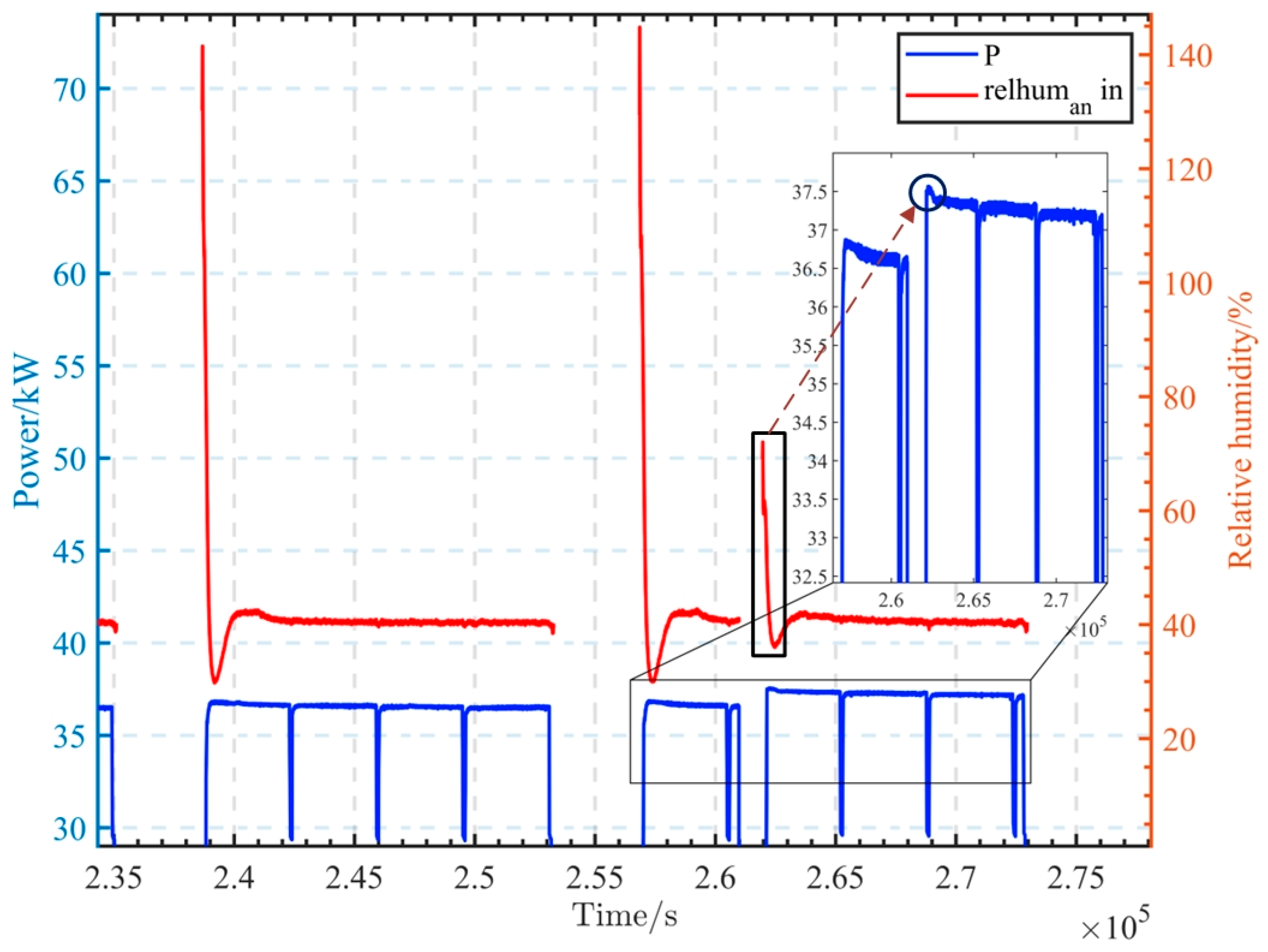
2.1. Fuel Cell Degradation Phenomena

Before predicting the decline trend of PEMFCs, the analysis of the degradation characteristics of PEMFCs is very important because the essence of this study is to determine the degradation-related factors of PEMFCs and predict them. Therefore, in this section, some previous work is referenced, and the decline phenomenon of FCs is analyzed [30,31,32,33,34,35]. During the whole operation of a PEMFC, all its components will degenerate or fail, leading to the decline of the PEMFC. The decline mechanisms of FCs often influence each other, and the primary causes for the degradation are the decline of the gas diffusion layer (GDL), the degradation of the catalyst layer, and the degradation of the polymer film. In addition, degradation mainly occurs in the MEA section.

The main phenomenon causing the decline of the GDL is carbon corrosion, which is often due to the high humidity and high potential of PEMFCs and the start–stop operation cycle [36]. Oxygen starvation, large changes in load, and other reasons will also accelerate performance decline.

In the catalyst layer, the important factor leading to the performance degradation is generally the dissolution or sintering of the catalyst particles. Because platinum particles are attached to carbon carriers, platinum particles easily fall off and gather when carbon corrosion occurs, while in acidic media, platinum is more likely to dissolve with increasing potential [37]. The shedding, migration, and accumulation of platinum will cause the loss of the ECSA [38].

In repeated chemical reactions, a polymer film is eroded and degraded [39]. Hydroxyl or hydrogen peroxide radicals are often produced in fuel cells under the conditions of high voltage, high temperature, and low humidity. These free radicals often come from hydrogen peroxide formed by fuel pollution or gas crossover. The free radical reacts with the end group of the polymer containing the terminal H group [40], resulting in the decomposition of the polymer to form HF. On the other hand, HF corrodes metals and forms metal cations to lead to the faster formation of free radicals. At the same time, due to the thinning of the polymer film, hydrogen can more easily penetrate into the cathode and accelerate the formation of free radicals, thus leading to a positive feedback loop and causing performance degradation.

In addition, the start–stop cycle will greatly affect the durability of the membrane electrode assembly (MEA). If FCs have a power outage for long, hydrogen will cross from the anode to the cathode so that the anode channel is filled with air. When in this state, starting the fuel cell will produce a transient operating condition, that is, although fuel is present at the entrance, there is a lack of fuel on the anode side of the exit. This local fuel shortage will cause the local potential of the cathode to be higher than 1.8 V, which will lead to serious degradation of the MEA [41].

In summary, many factors, including temperature, current, voltage, humidity, potential cycle, load change, start–stop condition, and fuel supply, will affect the degradation of PEMFCs.

It is worth noting that most of these factors are combined with each other, and there are still many factors that cannot be quantified, but can only qualitatively analyzed, so it is difficult to separate these factors to discuss the phenomenon of degradation. This is why many current model-based fuel cell degradation predictions are based on engineering empirical or semiempirical models rather than mechanism models. Therefore, regarding a fuel cell stack as a “black box” and using the external characteristic data-driven method to study its degradation characteristics has increasingly become an important method to establish a PEMFC degradation model.

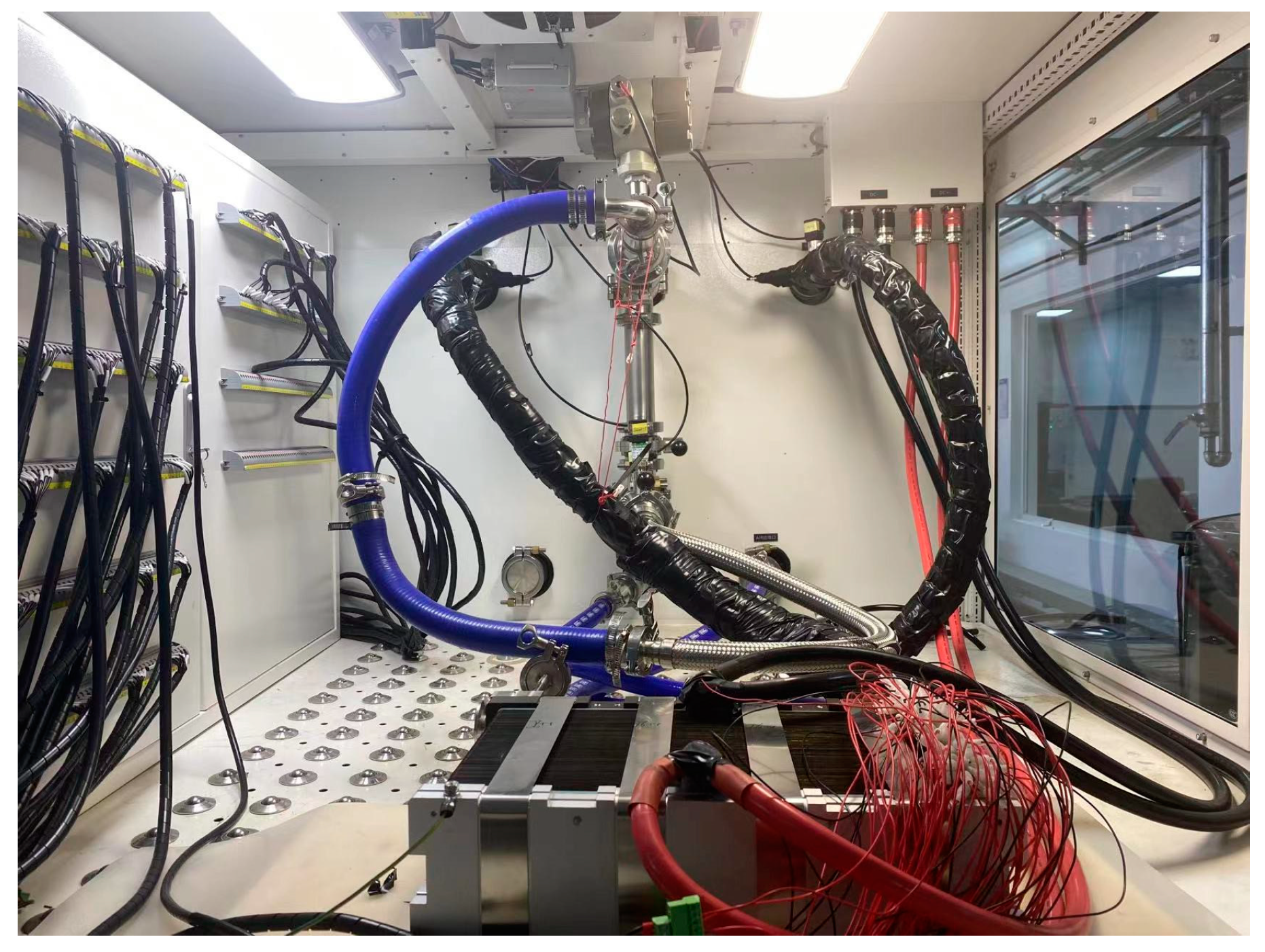
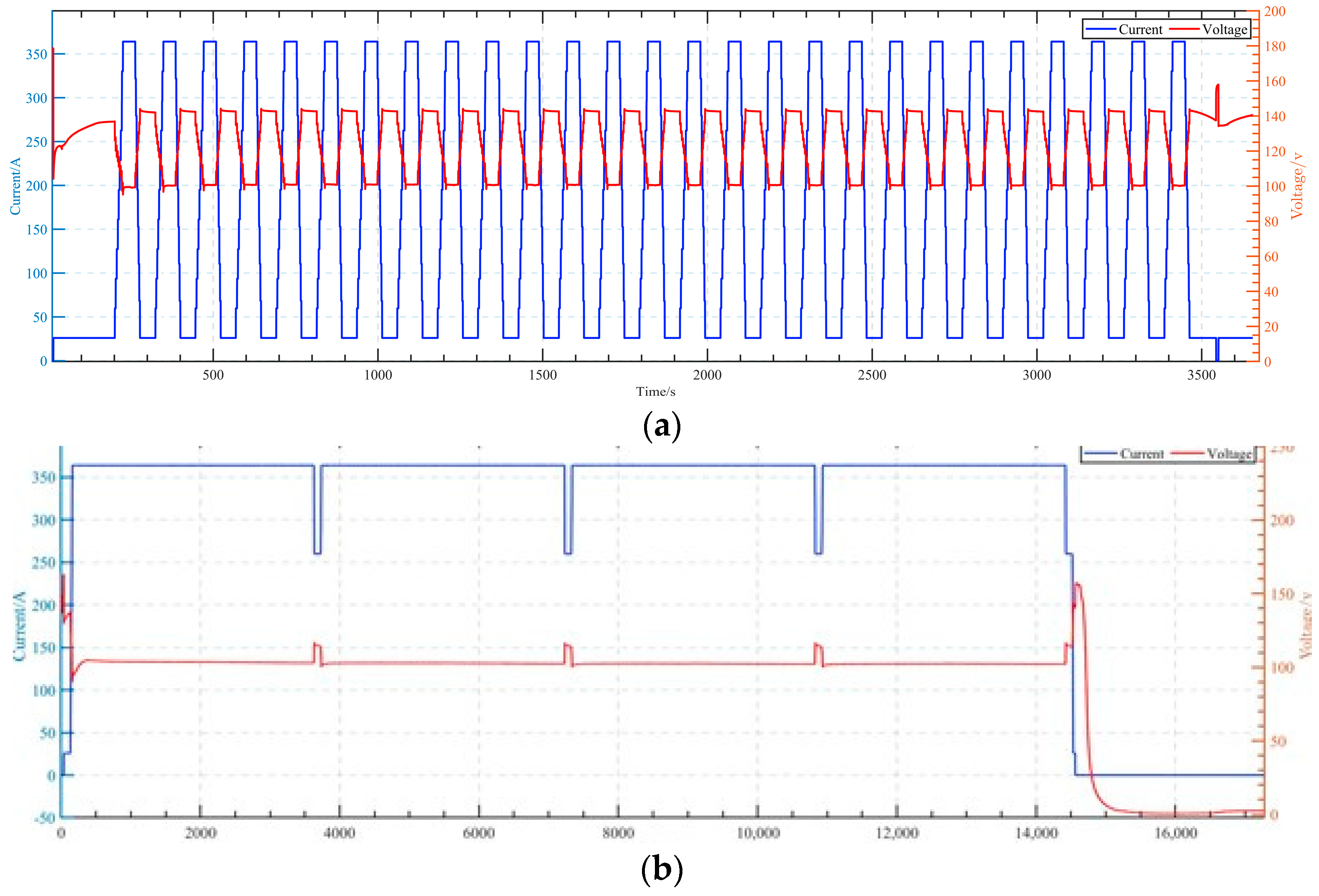
2.2. Aging Experiments for the Fuel Cell

The aging test was carried out with a 37 kW H2 core35 fuel cell stack containing 162 cells. The test bench is exhibited in Figure 1. This test was conducted at the Xiangyang Da’an Automobile Testing Center. The fuel cell was operated under the dynamic load conditions of stability assessment and rated conditions, as shown in Figure 2.

The stability test condition (FC1) was run for 340 h according to Figure 2a, and the sampling interval was 0.5 s. The working condition spectrum was as follows: start and stop once per hour, load 27 times, idle condition for 21 min, and rated condition for 18 min. After every 4 h of operation, the fuel cell stack was stopped and rested for 1 h. The rated state test (FC2) was run for 75 h with a sampling interval of 0.5 s, including the start-up, idle condition, rated current condition, reference current condition, and idle-stop condition. The test cycle is shown in Figure 2b. A test cycle was completed every 4 h, and after each cycle, the fuel cell stack was stopped for 1 h.

For this paper, stability assessment condition data were selected to train the fuel cell degradation model. Then, the prediction performance of the model was further verified with the data from the rated test conditions.

3. Degradation Model with an ACO-LSTM Architecture

This section, firstly, describes how the data directly obtained through the sensor were processed to eliminate specific points and enhance the characteristics of the degradation trend. In addition, it explains how the LSTM was improved to train the decline prediction model. Then, we will discuss the principle of the ACO method. Thus, a data-driven prediction model based on ACO-LSTM was developed for fuel cell degradation prediction.

3.1. Data Acquisition and Processing

In general, in the course of operation, the data directly obtained through the sensor are rarely directly used as training data, because these data often contain a lot of unexpected information, such as noise, downtime, specific points, and so on.

Therefore, after obtaining the original data, the first step is to resample and filter the data. As a finite impulse response (FIR) digital filter, a Savitzky–Golay (SG) filter smooths original time-domain signals based on local polynomial least-square fitting in the time domain. The most important feature of this method is that it can maintain the same signal structure as that of the original data after filtering. In this work, the SG filter [42] was used to eliminate the noise in the original data. The main parameters of the SG filter are the order of the polynomial and the length of the filter window [43].

The order of the polynomial and the window length of the SG filter were set to 2 and 20, respectively. The health state of the fuel cell has been defined in the previous text as its ability to guarantee sufficient power. Therefore, the degradation of the fuel cell’s health status can be represented by the power reduction, as shown in Equation (1):

$$P_{\mathit{drop}}=\frac{{P-P}_{\mathit{init}}}{P_{\mathit{init}}}\times 100\%$$

(1)

This formula represents the percentage drop in power, where $P_{\mathit{drop}}$ is the percentage decrease in power, $P$ is the current power, and $P_{\mathit{init}}$ is the initial power.

Therefore, the degradation of the PEMFC’s health status can be characterized by predicting the decay in power. However, under different operating conditions, especially in dynamic situations, defining an appropriate power value to characterize the health status is complex, because the power is not fixed but fluctuates within a certain range. Therefore, we chose to use the peak power $P_{\mathit{peak}}$ under the current condition for description:

$$Healt{h}_{FC,decline}=P_{peak,drop}=\frac{P_{peak}-P_{peak,init}}{P_{peak,init}}\times 100\%$$

(2)

In this formula, $Healt{h}_{FC,decline}$ represents the degradation of the fuel cell’s health status, $P_{peak,drop}$ represents the reduction in the fuel cell’s peak power, $P_{\mathit{peak}}$ represents the current peak power of the fuel cell, and $P_{peak,init}$ represents the peak power of the fuel cell in its initial state.

Therefore, the decline of the PEMFC is defined as the decline of peak power in this paper. The power envelope data under the condition of stability evaluation were selected in this study, and Figure 3 shows the data before and after filtering.

3.2. LSTM Architecture

An LSTM recurrent neural network is a special RNN. Its main advantage is that it can avoid the gradient disappearance and explosion of traditional neural networks in the process of long-sequence training. Its structure is shown in Figure 4. Unlike the traditional RNN, which has only one transfer state $C^{(t)}$, the LSTM RNN has two transport states, a cell state ($C^{(t)}$) and a hidden layer state ($h^{(t)}$). Among them, the update of $C^{(t)}$ adds some information on the bias of the previous state $C^{(t-1)}$, and the change range is very small. In contrast, $h^{(t)}$ makes large updates between different nodes. The main difference between the LSTM RNN and the traditional RNN is the improvement of the “gate” structures, such as the forget gate, input gate, and output gate. The gate structure is a sigmoid unit. Another key aspect of the LSTM, the internal state $S^{(t)}$, which is the core of each linearly activated neuron, can be seen as a carrier for adding or deleting information, in which the control of information flow is realized by the “gate” structure.

(1)

Forget gate: the first step of the LSTM algorithm is to selectively discard part of the information with the forget gate. It receives the inputs of $C^{(t)}$ and ${\mathrm{h}}^{(t)}$, then outputs a number between 0 and 1 to the internal state ${\mathrm{s}}^{(t)}$, where 1 represents the fully reserved state and 0 indicates complete discarding.

$$f^{(t)}=\sigma (W^{fc}{C}^{(t)}+W^{fh}{h}^{(t-1)}+b_f)$$

(3)

(2)

Input gate and input node: the second step is to decide which information to store in the internal state. This step needs to be completed in two small steps. First, the input gate ^(t) determines which values to update; then, a candidate state $\stackrel{\wedge }{S^{\left(t\right)}}$ is created by the input node $g^{(t)}$:

$$i^{(t)}=\sigma (W^{ic}{C}^{(t)}+W^{ih}{h}^{(t-1)}+b_i)$$

(4)

$$g^{(t)}=\tanh (W^{gc}{C}^{(t)}+W^{gh}{h}^{(t-1)}+b_g)$$

(5)

Thus, Equations (3)–(5) can update the old internal state ${\mathrm{s}}^{(t-1)}$ to $s^{(t)}$.

$${\mathrm{o}}^{(t)}=\sigma (W^{\mathrm{o}c}{C}^{(t)}+W^{\mathrm{o}h}{h}^{(t-1)}+b_o)$$

(6)

(3)

Output gate: the output gate determines what information to output.

$${\mathrm{o}}^{(t)}=\sigma (W^{oc}{C}^{(t)}+W^{\mathrm{o}h}{h}^{(t-1)}+b_o)$$

(7)

Finally, the hidden layer status is updated by combining the output door and the new internal state.

$$h^{(t)}=\tanh s^{(t)}\times o^{(t)}$$

(8)

Moreover, $w$ and $b$ are weights and biases, respectively, and their superscripts correspond to the corresponding relations. For example, $w^{\mathit{fc}}$ are the weights of the forget gate corresponding to $C^{(t)}$, and $b_f$ are the biases of the forget gate.

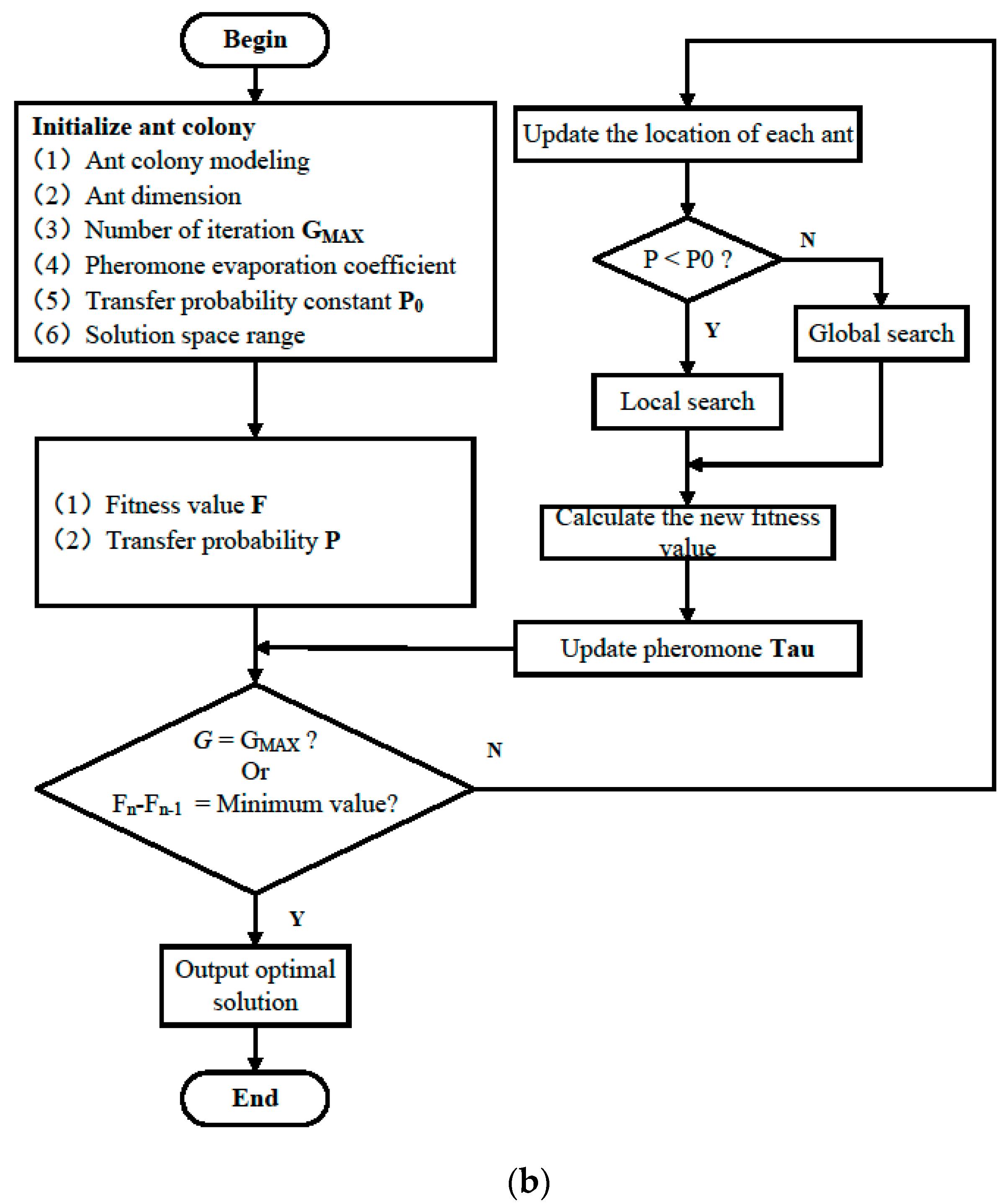
3.3. Structure and Implementation of ACO

The ACO is a kind of swarm intelligence algorithm, which is often used to solve optimization problems. In the ACO, there is a group of ants. “Nest” represents the nest, “Food” represents the food, and obstacles are randomly distributed on the map. The group of ants sets out randomly from the nest and gradually spreads all over the map until food is found. Then, the ants begin to move between the Nest and the Food. If an obstacle suddenly appears in front of an ant, the ant must make a decision about which direction to move in. Because there are no pheromones left by the first ants on the road, ants are equally likely to travel in any direction. However, when an ant is walking on the road, it releases pheromones on the road, and the pheromones are released at a certain speed. The pheromone is one of the tools for communication between ants, and it is also the core parameter of ant colony algorithm optimization. Each ant makes a decision and determines the direction of action based on the concentration of pheromones left on the road by the previous ants. Obviously, the pheromones along the shortest route will become increasingly thicker, attracting an increasing number of ants to walk along this path.

This kind of population intelligence behavior is transformed into a mathematical equation. Suppose there are M ants on the whole map, and the movement dimension of each ant is D, then, the location of ant $i$ is $X_i=(x_{i1}, x_{i2}, \dots , x_{\mathit{iD}},)$. Then, the transfer probability is shown in Equation (9) as follows:

$$P(G,i)=\frac{\max (Tau)-Tau(i)}{\max (Tau)}$$

(9)

where $\max (Tau)$ represents the maximum value of the pheromone, $Tau(i)$ represents the pheromone of ant $i$, and $P(G,i)$ represents the transfer probability value of ant $i$ in the $G$th iteration. When the transfer probability P is less than the transfer probability constant P₀, a local search is performed, and the search is shown in Equation (10):

$$\mathit{New}=\mathit{Old}+{\gamma }_1\times \mathit{step}\times \lambda$$

(10)

where $new$ is the position to be moved to, $old$ is the current position of the ant, r₁ is a random number from [−1,1], step is the local search step, and λ is the reciprocal of the current iteration number.

When P > P₀, a global search is performed, and the search formula is shown in Equation (11):

$$New=Old+r_2\times \mu$$

(11)

where r₂ is a random number in [−0.5, 0.5] and μ is the range of the solution space.

In defining the position of an ant within the range of values, whether or not to update the current position of the ant will be determined by judging the value of the objective function of the position to be moved to and the value of the objective function of the current position, and the boundary condition will be processed by using the boundary absorption method. The pheromone value for the new ant location is then set as follows:

$$Tau(i)=(1-Rho)\times Tau(i)+f$$

(12)

3.4. Dropout

At present, the commonly used methods to prevent neural network overfitting are the L1 and L2 regularization methods. Both methods rely on adding an extra term to the cost function, and this term can also be regarded as a penalty term of the loss function, which is used to limit some parameters in the loss function. In 2014, dropout technology was introduced by Srivastava et al. [44] to address the problem of overfitting more effectively.

The core of this method is to randomly delete some neurons and their connections temporarily (only before the next iteration) in the training process, as shown in Figure 3, and then randomly delete them in the next iteration so that each iteration trains a different network. The probability of deleting neurons is P (the probability between neurons is independent of each other). This approach is equivalent to sampling a “sparse” network in the original network. Thus, the training of the whole network is able to be seen as training multiple “samples”, so the completely unchanged network can avoid being trained repeatedly. Therefore, the whole network is no longer very sensitive to the specific weights of neurons. At the same time, this approach can also enhance the generalizability.

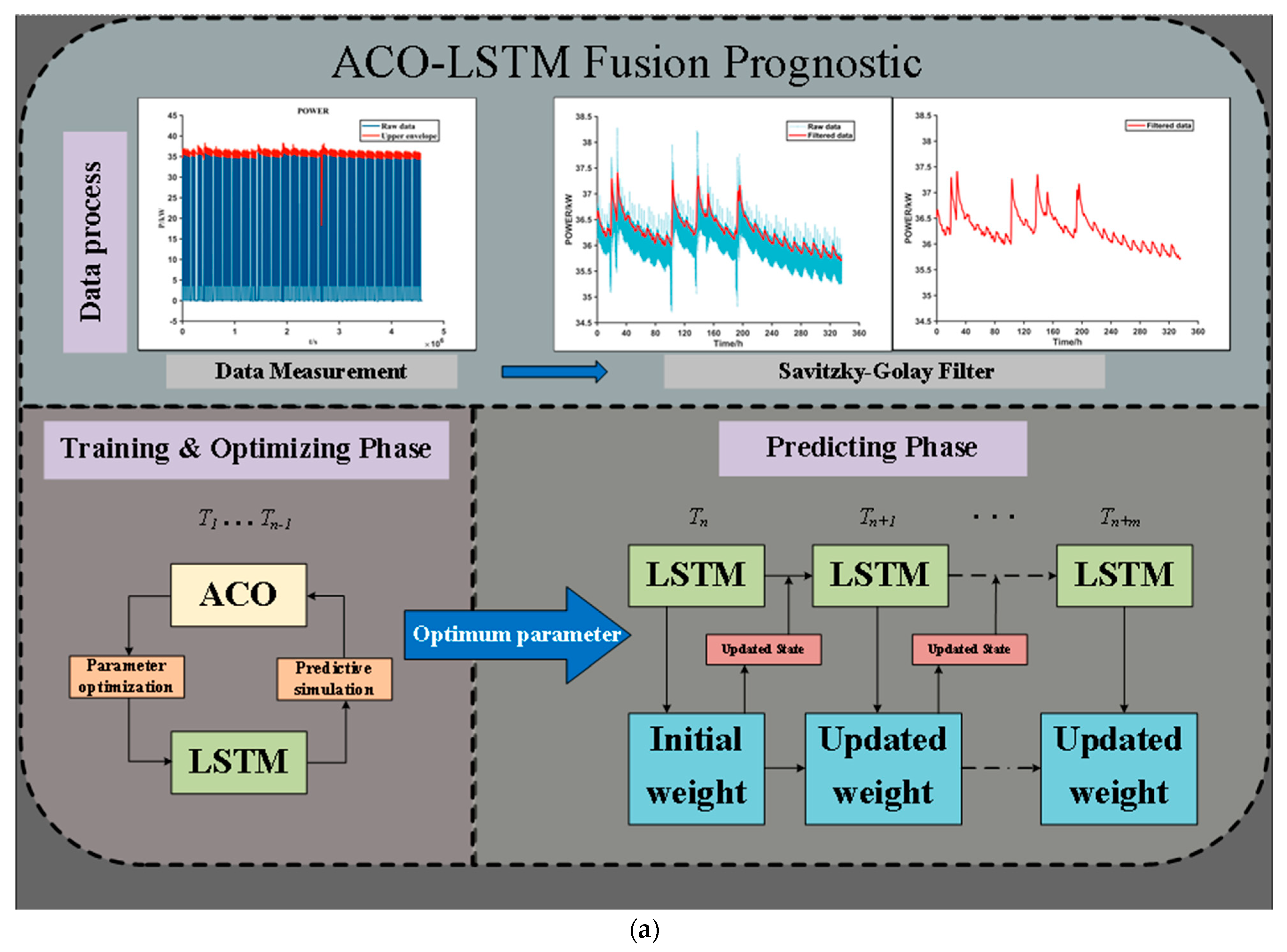
3.5. ACO-LSTM Approach

The previous sections of this paper analyzed the advantages and disadvantages of the traditional LSTM approach. The conventional LSTM method performs exceptionally well in long-term forecasting, for instance, it can prevent issues like gradient explosion and vanishing, and it is capable of retaining a moderate number of old experiences during training, rather than completely ignoring the impact of past experiences on the future. However, as a type of neural network, the setting of hyperparameters has a significant impact on LSTM training and forecasting performance. To some extent, improper hyperparameter settings can lead to the complete failure of the neural network. Existing studies often set key parameters based on prior experience or through continuous trial and error, but these methods can lead to numerous problems, such as being time consuming and labor intensive, leading to uncertainty about whether the parameter settings are appropriate, and fixed parameter settings based on different data characteristics and data volumes can lead to inappropriate parameters or even complete inapplicability. To address this, our study introduces the ACO (ant colony optimization) method to adaptively optimize the hyperparameters of the LSTM network, ensuring outstanding performance across different data characteristics and data volumes.

The ACO-LSTM method used in this study effectively combines the advantages of both approaches. It not only retains the excellent training and forecasting performance of the LSTM but also adaptively optimizes its key parameters. This prediction method can be divided into three independent parts, which are described in Figure 4a. The upper part corresponds to the selection and processing of data. The second part located at the bottom left is the ACO module, which can optimize the LSTM parameters. The last part, which is at the bottom right, is the prediction process.

The flowchart of the ACO-LSTM method is shown in Figure 4b, and the more specific implementation measures are listed as follows:

(1)

After the dataset is initially divided into a training set and a prediction set, the training set is subdivided into an LSTM simulation training set and an ACO optimization set.

(2)

The ACO algorithm is initialized, and a two-dimensional (initial learning rate, dropout probability) ant population is randomly generated.

(3)

The LSTM simulation training set is used as the training set, and the ACO optimization set is used as the test set to simulate the LSTM prediction process and let the ant with the smallest prediction error (defined as the RMSE in this paper) produce the densest pheromone in each iteration.

(4)

When the end condition is satisfied, the ant with the smallest historical error is selected as the optimal solution. Then, the optimal initial learning rate and dropout probability are obtained from this solution and are used to obtain the prediction results.

4. Degradation Prediction Results

4.1. Criteria of Predictive Performance

In this study, the mean absolute percentage error (MAPE), the root mean square error (RMSE), and the coefficient of determination (R²) are used to represent the prediction performance of the degradation model. Smaller MAPE and RMSE values indicate a more accurate prediction with lower errors. In contrast, the larger the R² value is, the better the prediction result is because it indicates the degree of agreement between the predicted data and the actual data. We can assume that in a perfect degradation prediction model, the MAPE and RMSE values are equal to 0, and the values of R² are 1:

$$\mathit{MAPE}=\frac{1}{N}{\displaystyle \sum _{i=1}^N\frac{\left|X_{\mathit{pre},i}-\left.X_{\mathit{obs},i}\right|\right.}{\left|X_{\mathit{pre},i}\right|}}$$

(13)

$$\mathit{RMSE}=\sqrt{\frac{{\displaystyle \sum _{i=1}^N(X_{pre.i}-X_{obs,i}{)}^2}}{N}}$$

(14)

$$R^2=1-\frac{{\displaystyle \sum _{i=1}^N(X_{pre.i}-X_{obs,i}{)}^2}}{{\displaystyle \sum _{\mathrm{i}=1}^N(\overline{X_{over}}-X_{obs,i}{)}^2}}$$

(15)

where X_pre represents the predicted power value, X_obs is the actual value of power, X_obs is the average of the actual power value, and N represents the total amount of data.

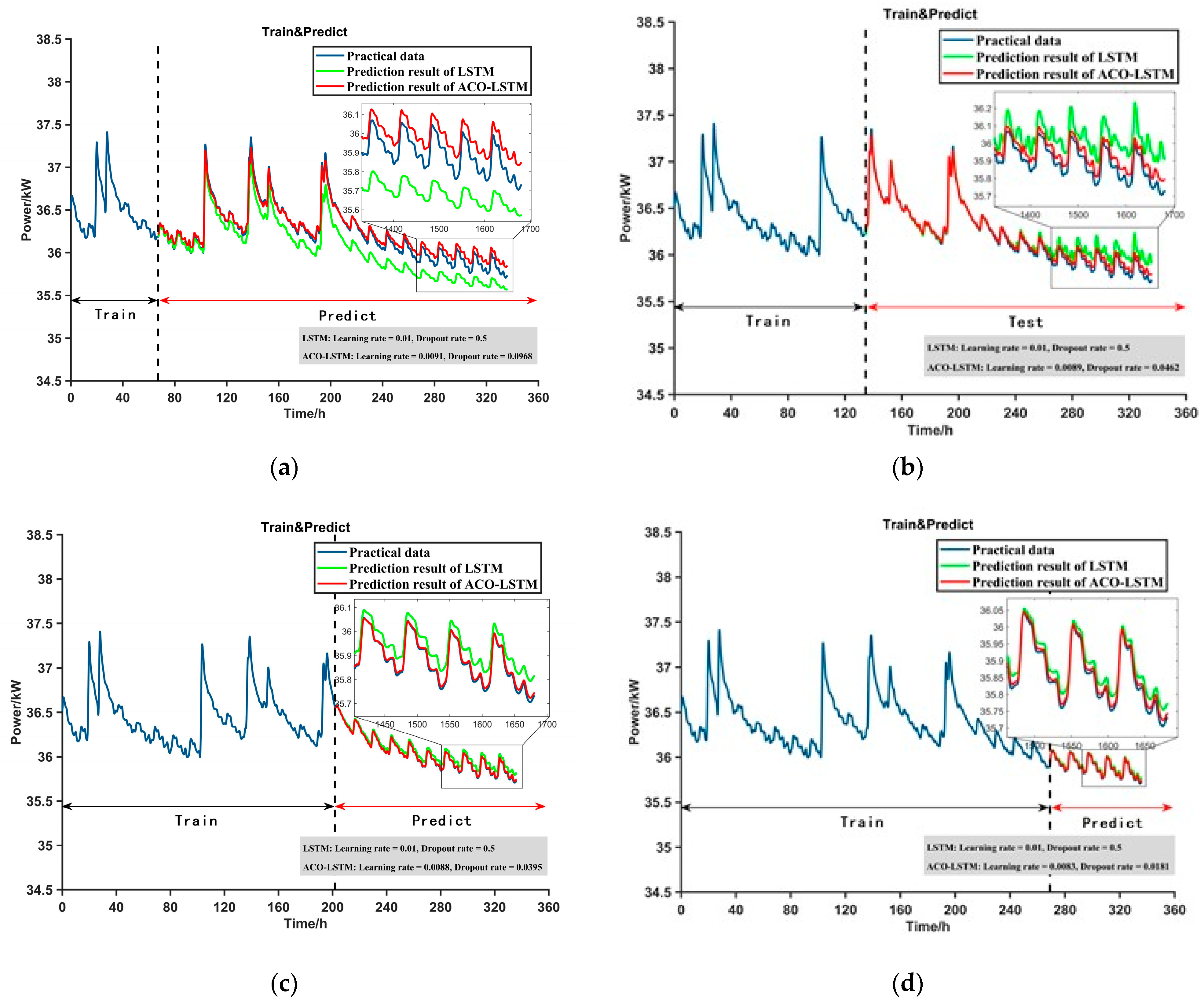
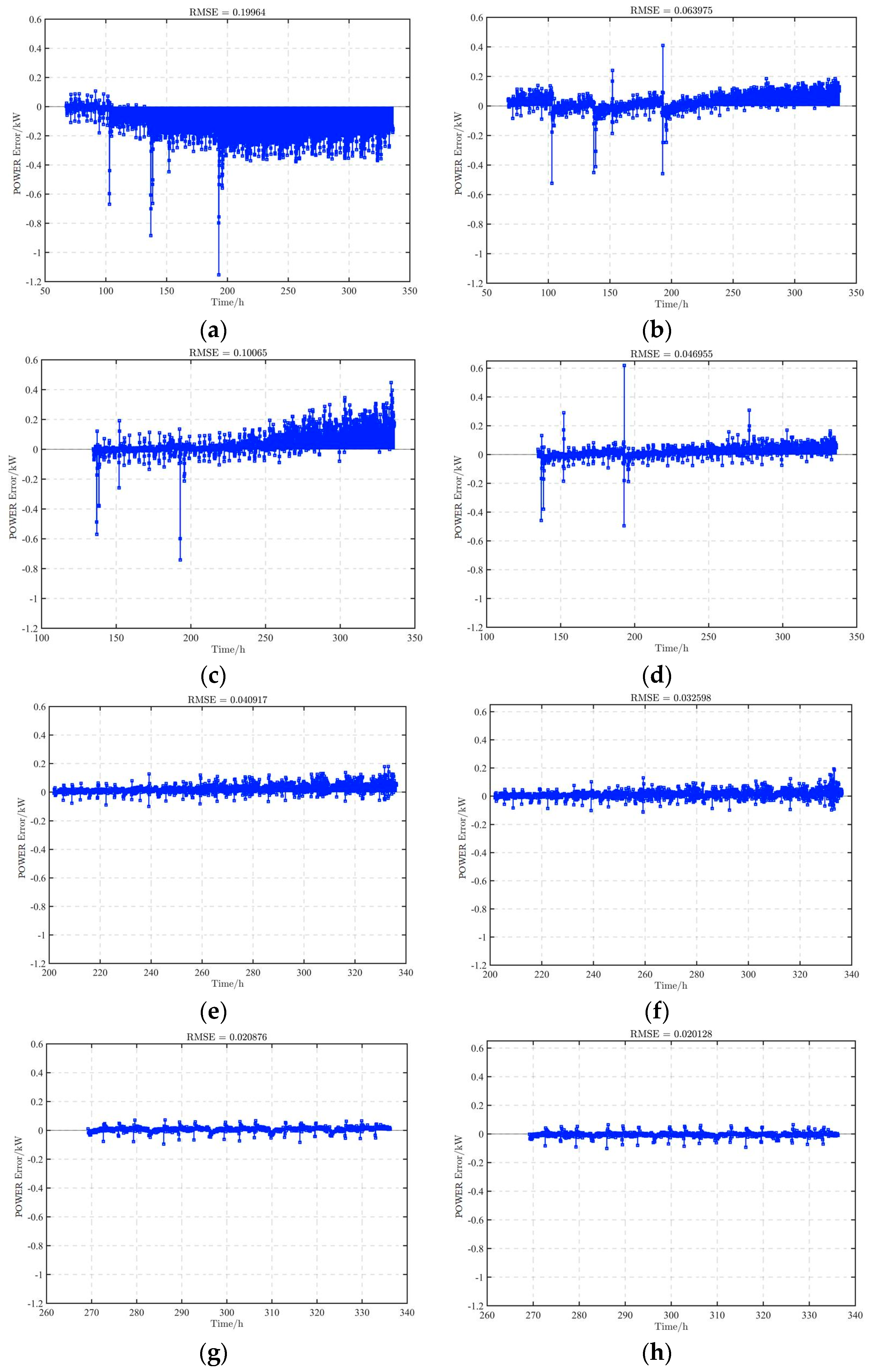
4.2. Degradation Prediction Model Based on ACO-LSTM

This section describes how the ACO-LSTM is trained with the FC1 (stability test) dataset and verified with the FC2 (rated test) dataset. It should be noted that FC2 did not participate in model training. The experiments of the two methods were based on CPU calculation and simulation. The LSTM RNN used in both groups consisted of an input layer, an LSTM layer (containing 100 hidden layer neurons), a fully connected layer, a dropout layer, and a regression layer. All used the Adam solver, and the total number of iterations was 100. In addition, 20%, 40%, 60%, and 80% of the dataset were selected for training (training data/total data) in both groups of experiments. In the first group, according to the recommendation in [27], the learning rate and the dropout probability were set as 0.01 and 0.5, respectively. The parameter settings of LSTM and ACO-LSTM were compared as shown in

Table 1. Comparison of the parameter settings between LSTM and ACO-LSTM.

	LSTM	ACO-LSTM
Hidden units	100	100
Solver	Adam	Adam
Iteration number	100	100
Learning rate decay algebra	50	50
Learning rate decay rate	0.2	0.2
Learning rate	0.01	Adaptive optimization
Dropout probability	0.5	Adaptive optimization

.

In this paper, the health status of FCs is defined according to the IEEE PHM 2014 data challenge [35] as the ability of a fuel cell stack to guarantee sufficient power at all times. Therefore, we use the peak power decay to indicate the health status of an FC stack.

Figure 5 shows a comparison of the prediction results of the LSTM method and the ACO-LSTM method under four different data proportions. In this figure, the blue curve is the actual power of PEMFCs, the green one is the power decline trend that is predicted using the LSTM, and the red curve represents the result predicted using the ACO-LSTM method.

Table 2. The learning rate and the dropout probability optimized using the ACO-LSTM method.

ACO-LSTM	20%	40%	60%	80%
Learning rate	0.0091	0.0089	0.0088	0.0083
Dropout probability	0.0968	0.0462	0.0395	0.0181

shows the learning rate and dropout probability obtained by using the adaptive optimization of the ACO-LSTM under different data ratios. In addition, the learning rate and dropout probability of the LSTM method remained at 0.01 and 0.5 under the four training data ratios.

As can be seen in Figure 5, the prediction accuracy of the decline prediction model trained using LSTM and ACO-LSTM increases with an increasing proportion of training data. The more training data are used, the more power degradation information the model will learn. According to the power RMSE error in Figure 6, the error increases gradually with time, regardless of which method is chosen. A single data-driven model always produces this result, and a solution is to introduce physical models for constraints. Although the error increase is inevitable, it is clear from

Table 3. Error assessment for LSTM and ACO-LSTM.

LSTM	20%	40%	60%	80%
MAPE	0.0049	0.0019	0.0008	0.0004
RMSE	0.1996	0.1007	0.0409	0.0209
R2	0.6328	0.9135	0.9604	0.9573
ACO-LSTM	20%	40%	60%	80%
MAPE	0.0014	0.0009	0.0007	0.0003
RMSE	0.0640	0.0470	0.0326	0.0201
R2	0.9623	0.9812	0.9774	0.9603

that the MAPE, RMSE, and R2 based on the ACO-LSTM method were all smaller than those of the traditional LSTM method. However, the gap between the ACO-LSTM method and the LSTM method was small at a high data ratio (60%, 80%), but was more significant at a low data ratio (20%, 40%). In particular, it is obvious that the LSTM method gradually lost different degrees of data traction for the power degradation curve, and the fitting accuracy of the prediction data was low. In contrast, although the ACO-LSTM method had a certain degree of error at low data ratios, it accurately tracked the degradation trend. Thus, it can be seen that the hyperparameters selected for the LSTM were more suitable for training the model under a high data ratio than under a low ratio, but the learning rate and dropout probability in [27] were selected on the basis of experience under the proportion of 25% training data, which is more suitable for a low ratio than a high ratio. This phenomenon further shows that different hyperparameters should be configured for diverse datasets and different proportions of training data.

4.3. Verification of the Degradation Prediction Model

To verify the predictive performance and generality of the trained model, the 60% data ratio training model was used to predict FC1 and FC2. As can be seen in Figure 7, the overall degradation trend of the fuel cell under dynamic load input was affected by the power recovery phase (power recovery to a certain extent after each shutdown restart). However, the ACO-LSTM still obtained the decline trend.

Brilliantly, for the whole prediction phase of FC1 and FC2, most of the errors between the target and the output were within 0.2 kW, which shows that the learning effect of the network is acceptable. It is worth noting that after 3321 s of FC2, the power degradation curve showed an abnormal jump, and the tracking effect of the prediction model decreased obviously. This was due to a short shutdown caused by a failure at 3321 s, and the anode inlet relative humidity control was not initialized during restart, as shown in Figure 8.

There was a more obvious downward trend in fuel cell power after 75 h under the rated test condition. For this condition, which is completely different from FC1, the proposed ACO-LSTM prediction network also performed well in the whole operating time range. The predicted output RMSE was 0.0471. The error distribution was within 0.2 kW most of the time, and within 0.4 kW after 3321 s. Thus, it can be concluded that the ACO-LSTM degradation model can achieve higher prediction accuracy of fuel cell aging.

Table 4. Error evaluation of the prediction results using the 60% data training model for LSTM and ACO-LSTM.

LSTM	FC1 (Stability)	FC2 (Rated)
MAPE	0.0006	0.0012
RMSE	0.0406	0.0564
R2	0.9857	0.9584
ACO-LSTM	FC1 (Stability)	FC2 (Rated)
MAPE	0.0005	0.0008
RMSE	0.0330	0.0463
R2	0.9905	0.9711

summarizes and compares the error assessment.

4.4. Conclusions

In this paper, a new data-driven method is proposed to predict the degradation trend of fuel cells, in which an LSTM network with ACO optimization is used to solve the problem of inappropriate setting of hyperparameters in the process of network training. And the dropout technology is introduced to avoid gradient disappearance or explosion during network training. Two different dynamic load conditions from the H2 Core35 fuel cell are used to train and verify the results of the prediction. At the same time, the traditional LSTM, which has the same setting but sets the hyperparameters according to experience, is compared with ACO-LSTM, which is introduced in this paper. The conclusions are as follows:

• The results show that ACO-LSTM can efficaciously train the high-precision degradation prediction model under different training data ratios and has a significant improvement compared with the traditional LSTM, especially in the case of a low data ratio.
• The proposed model shows good prediction performance in working conditions that are completely different from the training conditions, which proves its excellent generalizability.
• However, when there is a large instantaneous change in the prediction data, the prediction model loses part of its tracking ability, although its performance is still better than that of the traditional LSTM.

This method can be used to predict the performance degradation of fuel cells and further determine the failure threshold, which is helpful to monitor the performance of FCs. Because of its simple construction, the proposed ACO-LSTM prediction model can be easily implemented online once it has been trained. The proposed method is also expected to be combined with a model-driven method to constrain the error and further improve the prediction accuracy and interpretability, which needs to be further solved in the following work.

References

1. Liu, D.; Lin, R.; Feng, B.; Yang, Z. Investigation of the effect of cathode stoichiometry of proton exchange membrane fuel cell using localized electrochemical impedance spectroscopy based on print circuit board. Int. J. Hydrogen Energy 2019, 44, 7564–7573. [Google Scholar] [CrossRef]
2. Silva, R.E.; Gouriveau, R.; Jemeï, S.; Hissel, D.; Boulon, L.; Agbossou, K.; Steiner, N.Y. Proton exchange membrane fuel cell degradation prediction based on adaptive neuro-fuzzy inference systems. Int. J. Hydrogen Energy 2014, 39, 11128–11144. [Google Scholar] [CrossRef]
3. Yuan, H.; Dai, H.; Wei, X.; Ming, P. Model-based observers for internal states estimation and control of proton exchange membrane fuel cell system: A review. J. Power Sources 2020, 468, 228376. [Google Scholar] [CrossRef]
4. Yan, S.; Yang, M.; Sun, C.; Xu, S. Liquid Water Characteristics in the Compressed Gradient Porosity Gas Diffusion Layer of Proton Exchange Membrane Fuel Cells Using the Lattice Boltzmann Method. Energies 2023, 16, 6010. [Google Scholar] [CrossRef]
5. Zhong, D.; Lin, R.; Jiang, Z.; Zhu, Y.; Liu, D.; Cai, X.; Chen, L. Low temperature durability and consistency analysis of proton exchange membrane fuel cell stack based on comprehensive characterizations. Appl. Energy 2020, 264, 114626. [Google Scholar] [CrossRef]
6. Lin, R.; Che, L.; Shen, D.; Cai, X. High durability of pt-ni-ir/c ternary catalyst of pemfc by stepwise reduction synthesis. Electrochim. Acta 2020, 330, 135251. [Google Scholar] [CrossRef]
7. Wang, Z.; Xie, Y.; Zang, P.-F.; Wang, Y. Energy management strategy of fuel cell bus based on pontryagin’s minimum principle. J. Jilin Univ. Eng. Technol. Ed. 2020, 50, 36–43. [Google Scholar]
8. Lin, R.-H.; Xi, X.-N.; Wang, P.-N.; Wu, B.-D.; Tian, S.-M. Review on hydrogen fuel cell condition monitoring and prediction methods. Int. J. Hydrogen Energy 2019, 44, 5488–5498. [Google Scholar] [CrossRef]
9. Keller, R.; Ding, S.X.; Müller, M.; Stolten, D. Fault-tolerant model predictive control of a direct methanol-fuel cell system with actuator faults. Control. Eng. Pract. 2017, 66, 99–115. [Google Scholar] [CrossRef]
10. Tang, W.; Lin, R.; Weng, Y.; Zhang, J.; Ma, J. The effects of operating temperature on current density distribution and impedance spectroscopy by segmented fuel cell. Int. J. Hydrogen Energy 2013, 38, 10985–10991. [Google Scholar] [CrossRef]
11. Vasilyev, A.; Andrews, J.; Jackson, L.; Dunnett, S.; Davies, B. Component-based modelling of pem fuel cells with bond graphs. Int. J. Hydrogen Energy 2017, 42, 29406–29421. [Google Scholar] [CrossRef]
12. Park, J.; Oh, H.; Ha, T.; Lee, Y.I.; Min, K. A review of the gas diffusion layer in proton exchange membrane fuel cells: Durability and degradation. Appl. Energy 2015, 155, 866–880. [Google Scholar] [CrossRef]
13. Chen, H.; Pei, P.; Song, M. Lifetime prediction and the economic lifetime of proton exchange membrane fuel cells. Appl. Energy 2015, 142, 154–163. [Google Scholar] [CrossRef]
14. Zhang, X.; Pisu, P. Prognostic-oriented fuel cell catalyst aging modeling and its application to health-monitoring and prognostics of a pem fuel cell. Int. J. Progn. Health Manag. 2020, 5. [Google Scholar] [CrossRef]
15. Li, Y.; Yang, F.; Chen, D.; Hu, S.; Xu, X. Thermal-physical modeling and parameter identification method for dynamic model with unmeasurable state in 10-kW scale proton exchange membrane fuel cell system. Energy Convers. Manag. 2023, 276, 116580. [Google Scholar] [CrossRef]
16. Hu, Z.; Xu, L.; Li, J.; Ouyang, M.; Song, Z.; Huang, H. A reconstructedfuel cell life-prediction model for a fuel cell hybrid city bus. Energy Convers. Manag. 2018, 156, 723–732. [Google Scholar] [CrossRef]
17. Lu, L.; Ouyang, M.; Huang, H.; Pei, P.; Yang, F. A semi-empirical voltage degradation model for a low-pressure proton exchange membrane fuel cell stack under bus city driving cycles. J. Power Sources 2007, 164, 306–314. [Google Scholar] [CrossRef]
18. Jouin, M.; Gouriveau, R.; Hissel, D.; Pera, M.C.; Zerhouni, N. Degradations analysis and aging modeling for health assessment and prognostics of PEMFC. Reliab. Eng. Syst. Saf. 2016, 148, 78–95. [Google Scholar] [CrossRef]
19. Ou, M.; Zhang, R.; Shao, Z.; Li, B.; Yang, D.; Ming, P.; Zhang, C. A novel approach based on semi-empirical model for degradation prediction of fuel cells. J. Power Sources 2021, 488, 229435. [Google Scholar] [CrossRef]
20. Deng, Z.; Chen, Q.; Zhang, L.; Zhou, K.; Zong, Y.; Liu, H.; Li, J.; Ma, L. Degradation prediction of pemfcs using stacked echo state network based on genetic algorithm optimization. IEEE Trans. Transp. Electrif. 2021, 8, 1454–1466. [Google Scholar] [CrossRef]
21. Liu, Z.; Xu, S.; Zhao, H.; Wang, Y. Durability estimation and short- term voltage degradation forecasting of vehicle pemfc system: Development and evaluation of machine learning models. Appl. Energy 2022, 326, 119975. [Google Scholar] [CrossRef]
22. He, K.; Mao, L.; Yu, J.; Huang, W.; He, Q.; Jackson, L. Long-term performance prediction of pemfc based on lasso-esn. IEEE Trans. Instrum. Meas. 2021, 70, 3511611. [Google Scholar] [CrossRef]
23. Zhu, W.; Guo, B.; Li, Y.; Yang, Y.; Xie, C.; Jin, J.; Gooi, H.B. Uncertainty quantification of proton-exchange-membrane fuel cells degradation prediction based on bayesian-gated recurrent unit. eTransportation 2023, 16, 100230. [Google Scholar] [CrossRef]
24. Hua, Z.; Zheng, Z.; Pahon, E.; Pera, M.-C.; Gao, F. Multi-timescale lifespan prediction for pemfc systems under dynamic operating conditions. IEEE Trans. Transp. Electrif. 2022, 8, 345–355. [Google Scholar] [CrossRef]
25. Morando, S.; Jemei, S.; Hissel, D.; Gouriveau, R.; Zerhouni, N. Proton exchange membrane fuel cell ageing forecasting algorithm based on echo state network. Int. J. Hydrogen Energy 2016, 42, 1472–1480. [Google Scholar] [CrossRef]
26. Wu, Y.; Breaz, E.; Gao, F.; Paire, D.; Miraoui, A. Nonlinear performance degradation prediction of proton exchange membrane fuel cells using relevance vector machine. IEEE Trans. Energy Convers. 2016, 31, 1570–1582. [Google Scholar] [CrossRef]
27. Ma, R.; Yang, T.; Breaz, E.; Li, Z.; Briois, P.; Gao, F. Data-driven proton exchange membrane fuel cell degradation predication through deep learning method. Appl. Energy 2018, 231, 102–115. [Google Scholar] [CrossRef]
28. Zuo, B.; Cheng, J.; Zhang, Z. Degradation prediction model for proton exchange membrane fuel cells based on long short-term memory neural network and savitzky-golay filter. Int. J. Hydrogen Energy 2021, 46, 15928–15937. [Google Scholar] [CrossRef]
29. Gouriveau, M.H.R.; Hissel, D. IEEE phm 2014 Data Challenge: Outline, Experiments, Scoring of Results, Winners. Tech. Rep. 2014. [Google Scholar]
30. Pukrushpan, J.T. Modeling and Control of Fuel Cell Systems and Fuel Processors. Ph.D. Thesis, University of Michigan, Ann Arbor, MI, USA, 2003. [Google Scholar]
31. Dong, S.; Luo, T. Bearing degradation process prediction based on the pca and optimized ls-svm model. Meas. J. Int. Meas. Confed. 2013, 46, 3143–3152. [Google Scholar] [CrossRef]
32. Chen, J.; Jing, H.; Chang, Y.; Liu, Q. Gated recurrent unit based recurrent neural network for remaining useful life prediction of nonlinear deterioration process. Reliab. Eng. Syst. Saf. 2019, 185, 372–382. [Google Scholar] [CrossRef]
33. Mao, L.; Jackson, L.; Davies, B. Effectiveness of a novel sensor selection algorithm in pem fuel cell online diagnosis. IEEE Trans. Ind. Electron. 2018, 65, 7301–7310. [Google Scholar] [CrossRef]
34. Pei, P.; Chen, D.; Wu, Z.; Ren, P. Nonlinear methods for evaluating and online predicting the lifetime of fuel cells. Appl. Energy 2019, 254, 113730. [Google Scholar] [CrossRef]
35. Revankar, S.T.; Majumdar, P. Fuel Cells: Principles, Design, and Analysis, Fuel Cells Principles, Design, and Analysis; CRC Press: Boca Raton, FL, USA, 2014. [Google Scholar]
36. Huang, S.Y.; Ganesan, P.; Jung, H.Y.; Popov, B.N. Development of supported bifunctional oxygen electrocatalysts and corrosion- resistant gas diffusion layer for unitized regenerative fuel cell applications. J. Power Sources 2012, 198, 23–29. [Google Scholar] [CrossRef]
37. Xing, L.; Hossain, M.A.; Tian, M.; Beauchemin, D.; Adjemian, K.T.; Jerkiewicz, G. Platinum electro-dissolution in acidic media upon potential cycling. Electrocatalysis 2014, 5, 96–112. [Google Scholar] [CrossRef]
38. Zhang, S.; Yuan, X.Z.; Hin, J.; Wang, H.; Friedrich, K.A.; Schulze, M. A review of platinum-based catalyst layer degradation in proton exchange membrane fuel cells. J. Power Sources 2009, 194, 588–600. [Google Scholar] [CrossRef]
39. Lim, C.; Ghassemzadeh, L.; Van Hove, F.; Lauritzen, M.; Kolodziej, J.; Wang, G.G.; Holdcroft, S.; Kjeang, E. Membrane degradation during combined chemical and mechanical accelerated stress testing of polymer electrolyte fuel cells. J. Power Sources 2004, 257, 102–110. [Google Scholar] [CrossRef]
40. Curtin, D.E.; Lousenberg, R.D.; Henry, T.J.; Tangeman, P.C.; Tisack, M.E. Advanced materials for improved pemfc performance and life. J. Power Sources 2004, 131, 41–48. [Google Scholar] [CrossRef]
41. Yuan, X.Z.; Hui, L.; Zhang, S.; Martin, J.; Wang, H. A review of polymer electrolyte membrane fuel cell durability test protocols. J. Power Sources 2011, 196, 9107–9116. [Google Scholar] [CrossRef]
42. Schettino, B.M.; Duque, C.A.; Silveira, P.M. Current-transformer saturation detection using savitzky-golay filter. IEEE Trans. Power Deliv. 2016, 31, 1400–1401. [Google Scholar] [CrossRef]
43. Wu, M.T.; Tsai, M.H.; Huang, Y.Z.; Islam, S.H.; Hassan, M.M.; Alelaiwi, A.; Fortino, G. Applying an ensemble convolutional neural network with savitzky golay filter to construct a phonocardiogram prediction model. Appl. Soft Comput. 2019, 78, 29–40. [Google Scholar] [CrossRef]
44. Srivastava, N.; Hinton, G.; Krizhevsky, A.; Sutskever, I.; Salakhutdinov, R. Dropout: A simple way to prevent neural networks from overfitting. J. Mach. Learn. Res. 2014, 15, 1929–1958. [Google Scholar]
Figure 1. H2 Core 35 37 kW fuel cell stack experimental platform.
Energies 17 00968 g001
Figure 2. Fuel cell stack test cycle. (a) FC1: stability assessment condition, (b) FC2: rated test condition.
Energies 17 00968 g002
Figure 3. Savitzky–Golay filtered data. (a) Upper envelope of original power data; (b) upper original data; (c) filtered data.
Energies 17 00968 g003
Figure 4. ACO-LSTM fusion prediction model. (a) ACO-LSTM fusion prognostic; (b) the flow chat of ACO-LSTM.
Energies 17 00968 g004aEnergies 17 00968 g004b
Figure 5. LSTM and ACO-LSTM degradation model prediction performance: (a) 20% dataset for training; (b) 40% dataset for training; (c) 60% dataset for training; (d) 80% dataset for training.
Energies 17 00968 g005
Figure 6. LSTM and ACO-LSTM degradation model prediction performance: (a) 20% dataset for training (LSTM); (b) 20% dataset for training (ACO-LSTM); (c) 40% dataset for training (LSTM); (d) 40% dataset for training (ACO-LSTM); (e) 60% dataset for training (LSTM); (f) 60% dataset for training (ACO-LSTM); (g) 80% dataset for training (LSTM); (h) 80% dataset for training (ACO-LSTM).
Energies 17 00968 g006
Figure 7. Prediction results of training model using 60% of FC1 data. (a) Forecast result of FC1; (b) forecast result of FC2.
Energies 17 00968 g007
Figure 8. Analysis of FC2.
Energies 17 00968 g008