Short-Term Prediction of the Intermediate Point Temperature of a Supercritical Unit Based on the EEMD–LSTM Method

Abstract

The quality of the intermediate point temperature control of a supercritical unit is directly related to the quality of the coal–water ratio and main steam temperature control of the supercritical unit, which is also related to the economy and safety of the unit. In order to improve the accuracy of short-term predictions of the intermediate point temperature, a short-term prediction model of the intermediate point temperature based on the EEMD (Ensemble Empirical Mode Decomposition)-LSTM (Long Short-Term Memory) model is proposed. This model uses the data of a 600 MW thermal power station in 2022 as a sample. The EEMD method is used to decompose the historical data into IMF components and residual components, and the correlation between each component and the original data is calculated. The relevant components are sent to the LSTM neural network, and all the sub-components are superimposed to obtain the final intermediate point temperature prediction results. At the same time, the BP and LSTM models are built to compare the errors with the proposed model. The results show that the single model will produce large errors when predicting the factors of large data fluctuations. The EEMD–LSTM coupling model can fully extract the detailed features and the prediction effect is obvious. The prediction accuracy of the EEMD–LSTM prediction model built in this paper is significantly better than that of the other two models. It has certain application value in the research field of intermediate point temperature prediction and can meet the requirements of short-term predictions of the intermediate point temperature.

1. Introduction

The intermediate point temperature of a supercritical boiler temperature is the temperature of the working fluid from the water wall to the outlet steam water separator. The intermediate point temperature is often used as the feed-forward signal of the main steam in the field. Through the introduction of a control system, the measures to prevent the film boiling or film boiling of the water wall are prevented, and the alarm signal of the water wall is protected [1]. The intermediate point temperature is affected by parameters such as the feed water, coal quantity, feed water temperature, total air volume and unit load. There is a strong coupling relationship between the above parameters and the intermediate point temperature, which cannot be described by a simple mechanistic model. It is easier to describe using a data-driven method. The main steam temperature has a great influence on the safety, stability and operation of the unit. In boiler emergencies, more than 50% of the accidents are caused by the overheating and overpressure of the superheated steam [2]. Because of the multi-internal DC form adopted by supercritical units, the complex of the steam–water system, the length of travel, and the changing model parameters with changing working conditions (especially the introduction of deep peak regulation), the working state of the steam–water system is extremely complicated. It is difficult for a controller designed according to the traditional object model to meet the control requirements [3]. It cannot be described by a simple mechanistic model, and it is easier using a data-driven method. In actual operation, the intermediate point temperature is controlled by adjusting the water–coal ratio through experimentation; however, the difference in the intermediate temperatures corresponding to the load of each unit results in hysteresis and errors in the regulatory control of the intermediate point temperature. Therefore, it is very important to establish an intermediate point temperature simulation model to guide the regulation control. With the increase in the installed capacity of the unit and the continuous improvement of the parameters, higher requirements are needed for the performance of the control system [4]. In-depth studies of the thermal object of a power plant unit and the establishment of a mathematical model are key to ensuring the control quality, and have always been the focus of research in the field of thermal process control. The study in [5] shows that in the 1960s, simulation technology was applied to the modeling of thermal systems. At present, many experts and scholars have used the mechanism model identification method to study the power station control system, and have achieved a lot of research results, and established many models and empirical formulas. The study in [6] used the recursive least squares method to develop a model for the superheated steam temperature system of a 330 MW subcritical unit, and on this basis, a two-stage superheated steam temperature linkage control optimization strategy was constructed by applying multivariate generalized predictive control. In [7], an improved particle swarm algorithm identification was used to obtain a mathematical model with three inputs and three outputs for a 600 MW supercritical unit, which was established a temperature model with a high accuracy. The study in [8] used partial least squares regression in conjunction with actual unit operational data to model a supercritical unit.

However, the identification method based on the mechanism model requires in-depth principle analysis of the controlled object and relies on an empirical formula to set the parameters. The accuracy and universality of the model are very poor, especially for a power plant with flexible transformation and deep peak shaving, where the impact is greater and the model’s adaptability is difficult to guarantee. With the development of artificial intelligence algorithms, data-driven modeling methods are becoming more and more mature. In particular, for thermal power plants, which have long-term continuous operation and accumulated massive data, data-driven modeling is very suitable. In the data-driven modeling method, neural network algorithms are a typical representative and are widely [9] used. As an adaptive pattern recognition technology, neural networks do not need empirical knowledge and a discriminant function of the model in advance. It can automatically form the required decision region through its own learning mechanism. The characteristics of the network depend on the topology of the neural network, the characteristics of the neurons, and the rules of learning and training [10]. Therefore, many experts and scholars have applied neural network algorithms to the control of thermal power units. In study in [11], the neural network identification method was used for training using a large amount of data to obtain a model of the main steam temperature system. The study in [12] proposed an identification method combining field data and mechanism analysis, and verified that the output of the model and the actual field output data have a high degree of fitting. The study in [13] proposed a steam temperature identification method combining field data and neural networks. The results show that the identified model met the accuracy requirements.

With the development of technology, deep learning has gradually replaced the traditional neural network as the representative of intelligent algorithms. Long Short-Term Memory (LSTM) is a kind of machine learning intelligent algorithm, which is widely used in signal modeling, time series prediction and other research which can effectively solve the series of gradient problems caused by RNNs. Many scholars have applied time series prediction methods to finance and business, computer science, agricultural engineering, power plant thermal systems, and many interdisciplinary fields [14]. In [15], a model prediction method based on the LSTM algorithm was proposed by identifying the real-time data [16]; it analyzed how windy weather can easily lead to high-speed train accidents and proposed a two-layer LSTM network structure, which was verified by using wind speed data in a certain area. The study in [17] analyzed the characteristics of wind speed with strong randomness and many influencing factors and proposed a wind speed prediction method based on LSTM. The studies in [18,19] described the application of deep learning in power-load forecasting, listed the commonly used deep learning algorithms, and after comparative analysis, verified that the LSTM (Long Short-Term Memory Neural Network) algorithm has high accuracy. In study in [20], the LSTM algorithm was applied to the study of pollutant emissions from power plants, and the correctness of the method was proven. In study in [21], the LSTM algorithm was introduced into the field of the prediction and identification of coal-fired boilers. The experiments showed that the convergence process of the model identified using LSTM was stable, and few time steps were required.

However, in terms of the prediction method for the intermediate point temperature, which is an important parameter of the main steam temperature control and the main feed water control, the combination of EEMD (Ensemble Empirical Mode Decomposition) and LSTM has been less used. EEMD can decompose various features contained in the intermediate point temperature time series data one by one, and the selection of the main IMF components is carried out, which can effectively avoid the phenomenon of modal aliasing [22], which is conducive to better prediction and an improvement in the prediction accuracy. LSTM is a good alternative model to the RNN, as it eliminates the risk of gradient disappearance and gradient explosion that may occur in RNN when processing time series [23]. When predicting without considering the underlying mechanism process, the LSTM model can be used as an alternative to the physical model to predict the change in the intermediate point temperature. The model has strong applicability and learning ability for data with high degree of nonlinearity, can compare and update memory information and current information more accurately and efficiently, and has a higher accuracy and better prediction ability than the traditional prediction methods [24]. For neural networks, state information can be fully utilized to train information from different states one by one to obtain a certain correlation mapping relationship. Due to the characteristics of the neural network itself, it has been widely studied and applied in the field of time series prediction.

The intermediate point temperature of a supercritical unit refers to the temperature of the working medium in the steam–water separator at the outlet of the water wall. In the supercritical pressure boiler, the temperature of the working fluid in the water wall changes with the change in the heat absorption, while the change in the temperature of the working fluid at the outlet of the water wall must first directly affect the superheated steam temperature. Therefore, the intermediate point temperature is obviously very important as the leading signal or the primary reference temperature for controlling the superheated steam temperature.

The intermediate point temperature is a function of the separator pressure, which needs to ensure that the steam in the separator is 10~30 °C. Based on the importance of the intermediate point temperature, the intermediate point temperature protection is set. Obviously, the quality of the coal directly affects the size of the water–coal ratio; for example, if the actual coal type has a higher calorific value than the designed coal type, the value of the water–coal ratio will be larger. Therefore, the water–coal ratio is only a coarse estimate of the intermediate point temperature.

At present, most of the research on the control model of the intermediate point temperature of a supercritical unit has difficulty in fully reflecting its dynamic characteristics. The model data are very different from the actual operating data, and it is difficult to apply in practice. A combined prediction model can indeed improve the prediction accuracy in the prediction of the intermediate point temperature time series. The use of EEMD does not require any subjective intervention; it provides a truly adaptive data analysis method. By eliminating modal aliasing, a set of IMFs that can carry the full physical meaning of each component is generated. These IMF components are able to more accurately characterize the local features of the original data at different time scales [25]. Moreover, LSTM consists of a forgetting gate, input gate, output gate, and cell state messaging part [26], creating good short-term prediction capability. From the literature review and analysis, few prediction studies were found in this field based on an EEMD and LSTM decomposition ensemble series combination model. Therefore, this paper attempts to construct an EEMD–LSTM decomposition and integration model for empirical analysis to explore its performance in the short-term prediction of an intermediate point temperature time series.

In this study, an intermediate point temperature identification method based on EEMD–LSTM is proposed. Firstly, the neural network is used to abstract the historical data for preprocessing to decompose the characteristic data and extract the variation law of the signal at different scales. Then, the data after EEMD decomposition are input into the LSTM identification algorithm for object modeling. The model has higher accuracy than the traditional prediction method. In order to improve the learning efficiency of the prediction model and extract the characteristics of the data, this work introduces the data processing method of data decomposition into the prediction and uses the EEMD signal decomposition method to extract the characteristics of the data on different time scales, so that the prediction accuracy can be further improved. By adjusting the structure and parameters of the algorithm, the intermediate point temperature system model is finally established.

2. Analysis of Input Influencing Factors

In the actual operation of a supercritical unit, the important parameters of the main steam temperature control and the wall temperature safety control are determined by the key variable of the intermediate point temperature, and there are many factors affecting the intermediate point temperature. As the main means to adjust the temperature of the intermediate point, the amount of water and coal can directly affect the temperature of the intermediate point. When the unit load is different, the intermediate point temperature will be different; thus, the relationship between the two is close. The total air volume can control the combustion and heat transfer of the furnace, which further affects the heat absorption of the water wall and then affects the intermediate point temperature. At the same time, the feed water temperature, as an advance control parameter for entering the water wall, indirectly affects the temperature of the intermediate point [27]. According to the relevant mechanism research and field operation experience, four feature vectors, including the coal quantity, water supply quantity, water supply temperature of the economizer outlet, and the total air volume of the furnace, were selected as inputs. Considering the change in the normal operation parameters of a boiler under different unit loads, the unit load was also used as an input neuron for the accuracy of the simulation training.

Based on the above analysis, it was reasonable to use the coal quantity, water supply quantity, water supply temperature of the economizer outlet, total air volume of the furnace, and the boiler load as prediction input data, which are shown in Figure 1. Some input and output data of the prediction model are shown in

Table 1. Access characteristics of the thermal equipment.

Serial Number	Feed Water Quantity (t/h)	Coal Quantity (t/h)	Unit Load (MW)	Feed Water Temperature (°C)	Total Furnace Air Volume (%)	Intermediate Point Temperature (°C)
1	849.206	162.533	328.516	600.4415	1224.46	363.171
2	845.906	162.282	329.573	600.4415	1226.206	364.171
3	843.209	162.459	329.111	600.4415	1227.82	364.171
4	842.526	162.226	329.903	600.3695	1229.516	364.025
5	840.602	162.226	329.243	600.298	1233.786	364.025
6	842.22	162.026	330.102	600.2265	1236.135	364.171
7	841.738	161.825	329.375	600.2265	1238.163	364.025
8	839.977	161.825	329.375	600.155	1236.797	364.025
9	839.596	161.825	330.696	600.011	1234.9	364.171
10	841.877	161.825	329.639	600.011	1231.505	364.171
11	842.23	161.825	329.639	600.011	1230.08	364.171
12	842.381	161.825	330.234	600.011	1233.341	364.317
13	842.806	161.825	328.78	600.011	1235.257	364.317
14	842.584	161.825	329.375	599.868	1232.022	364,463
15	844.239	161.825	328.846	599.9395	1235.836	364.609
16	843.355	161.825	328.639	599.9395	1235.629	364.754
17	844.658	161.825	330.102	599.7965	1230.513	364.9
18	844.679	161.633	329.045	599.868	1227.551	364.9
19	843.926	161.633	328.582	599.7965	1228.61	365.046
20	843.365	161.633	329.111	599.7965	1221.381	365.046

. The intermediate point temperature of a supercritical once-through boiler is used as the output neuron. Due to the strong coupling and nonlinear characteristics among neurons, it is difficult to describe it with a simple mechanism model. The EEMD–LSTM neural network can be arbitrarily approximated to nonlinear functions and dynamic systems. Therefore, this model was used to establish the intermediate point temperature prediction model.

3. EEMD and LSTM Prediction Methods

When the output data of the intermediate point temperature fluctuate, the parameters of the model will change accordingly, and the accuracy of the prediction model will be affected. Therefore, it is necessary to use EEMD to decompose the historical data to ensure the accuracy of the model.

3.1. EEMD Decomposition

The EEMD decomposition aliasing method is mainly designed to optimize the mode-aliasing phenomenon similar to the Empirical Mode Decomposition method; EEMD is an improvement on the EMD method, which is a method of assisting in the decomposition of the data through the inclusion of noise signals [28]. The Empirical Mode Decomposition (EMD) method can decompose the different scale components in any time series signal in turn and generate multiple sets of data sequences with different scale features; each set of data sequences is an intrinsic mode function (IMF) [29]. Firstly, white noise is added to the input signal, and then EMD decomposition is performed. The mean value of the IMF component after multiple decompositions is calculated [30], and an original input signal $x\left(t\right)$ is given. Adding Gaussian white noise to the original signal effectively improves the mode aliasing problem. Since the EEMD method is based on the EMD method, the decomposition frequency $m$ of EMD and the amplitude k of the Gaussian white noise will directly affect the accuracy of model prediction.

Before using EEMD, the integrated average number m and the amplitude k of the added white noise need to be initialized, where σ is the standard deviation of the original signal.

$$\ln \sigma +\frac{k}{2}\ln m=0$$

(1)

$$k=0.2\sigma$$

(2)

After several parameter adjustments, the m value was finally determined to be 150 and the k value to be 0.25.

The EEMD decomposition process is as follows:

(1)

Add normal Gaussian noise with amplitude k = 0.25 into the signal, set the number of EMD decomposition $m$ as 150, and set the number of iterations m as 1.

(2)

Carry out the m-th iteration of the Empirical Mode Decomposition (EMD). The EMD decomposition process is as follows:

➀

After adding Gaussian white noise to the data series of the intermediate point temperature, the new data series is as follows:

$$x_m\left(t\right)=x\left(t\right)+k{q}_m\left(t\right), m=1,\cdots ,k$$

(3)

In the formula:

$x\left(t\right)$—raw data series of the intermediate point temperature;

$m$—the number of times white noise is added;

$q_m\left(t\right)$—white Gaussian noise;

$x_m\left(t\right)$—new temperature series.

➁

The new temperature series $x_m\left(t\right)$ is decomposed by EMD to obtain n IMF components and one remaining component:

$$x_m(t)={\sum }_{i=1}^n{C}_{mi}(t)+R_m\left(t\right)$$

(4)

  In the formula:

  $C_{mi}\left(t\right)$—the m-th decomposition yields the i-th component of the IMF;

  $R_m(t)$—remaining component.

(3)

Compute the average of each individual decomposed quantity:

$$C_i(t)=\frac{1}{k}{\sum }_{m=1}^k{C}_{mi}(t)$$

(5)

  $C_i\left(t\right)$ represents the ultimate outcome of the decomposition process.

3.2. LSTM Algorithm

Long Short-Term Memory (LSTM) [31] is a kind of machine learning intelligent algorithm, which is widely used in signal modeling and time series prediction and can effectively solve a series of gradient problems caused by the recurrent neural network RNN.

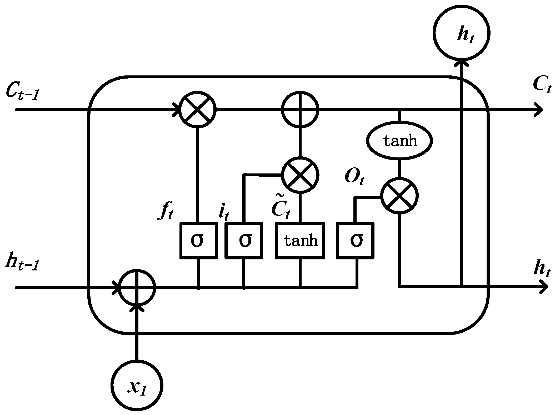
As with the traditional RNN networks, LSTM topological neural networks are also composed of a combination of an input control layer, an output control layer, and a hidden layer. Compared with traditional RNN networks, the hidden layer of LSTM neural networks uses gated memory modules to replace ordinary input neurons, whose topology is shown in Figure 2. The gated memory module unit is the most important core component of the LSTM system structure, and its memory state at a certain moment $t$ is recorded as $c_t$, which includes part of the long-term memory data information of the memory sequence. The memory state $h_t$ of the hidden layer at a certain moment $t$ mainly contains some short-term memory data information of the memory sequence. Obviously, the former memory data cycle update rate is much lower than the latter. The whole memory module is realized through an input gate, an output gate, and a forget gate.

At a specific moment, the input of a memory unit module in LSTM mainly includes the sequence input $x_t$, the state $h_{t-1}$ before the hidden layer, and the state $c_{t-1}$ before the memory unit. The sequence output of the memory unit module mainly includes the state of the hidden layer $h_t$ and the state of the memory unit $x_t$ at this moment. The influence degree of the input gate control is $x_t$ on $c_t$; the influence of $c_t$ on $h_t$ is controlled by the output gate. The forgetting door is mainly responsible for controlling and processing the historical data information in the memory unit.

3.3. The EEMD–LSTM Model

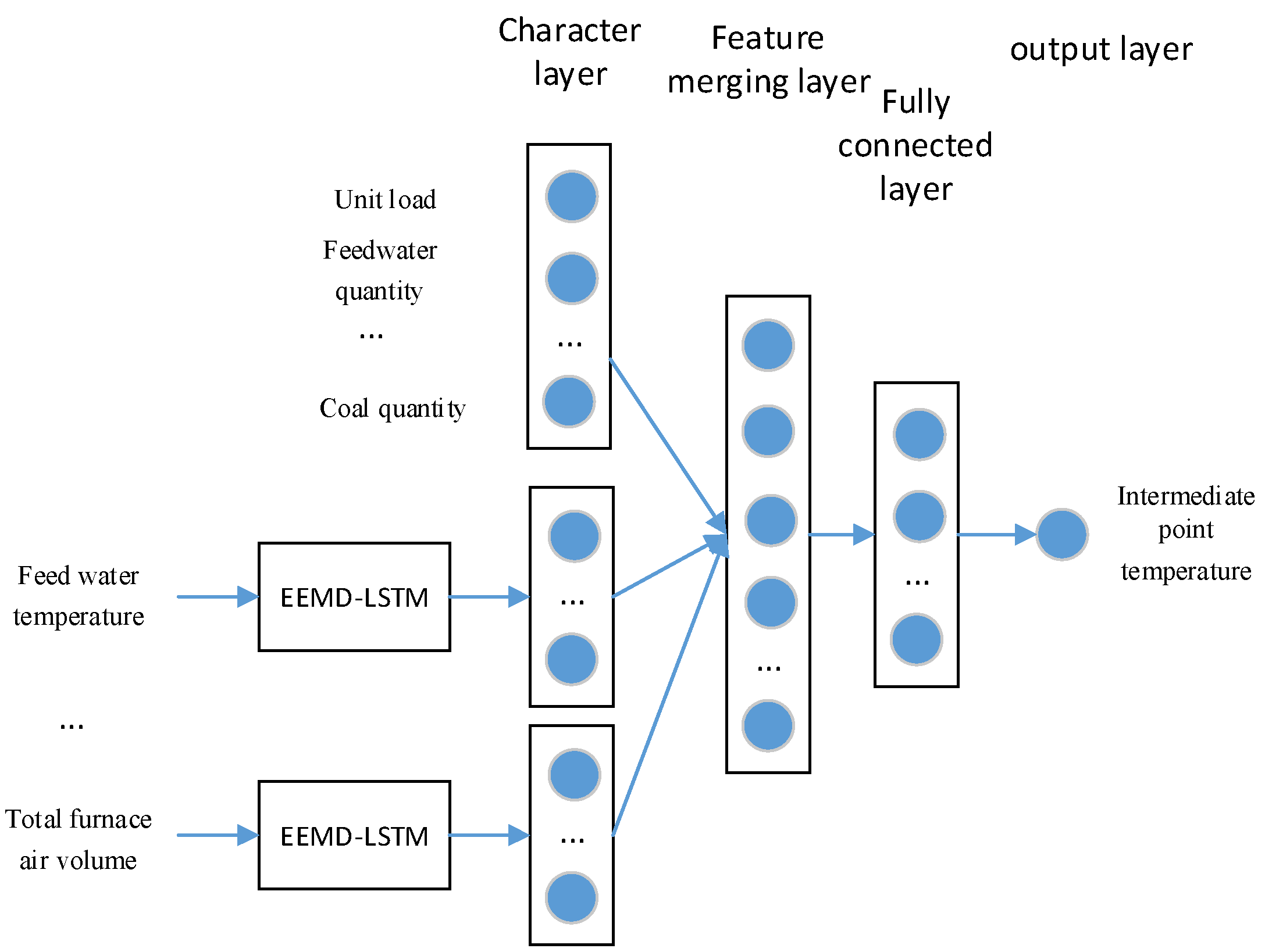
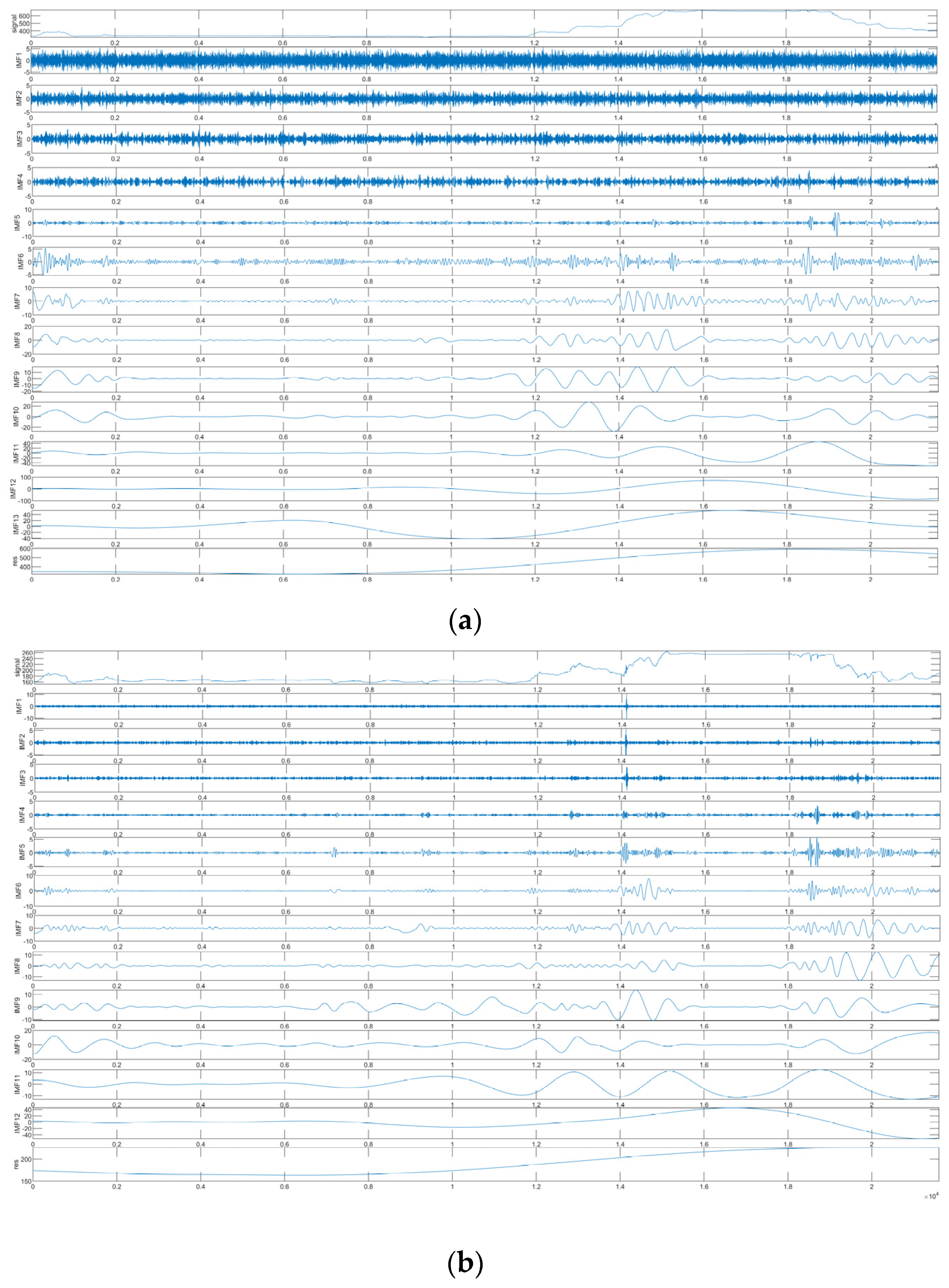
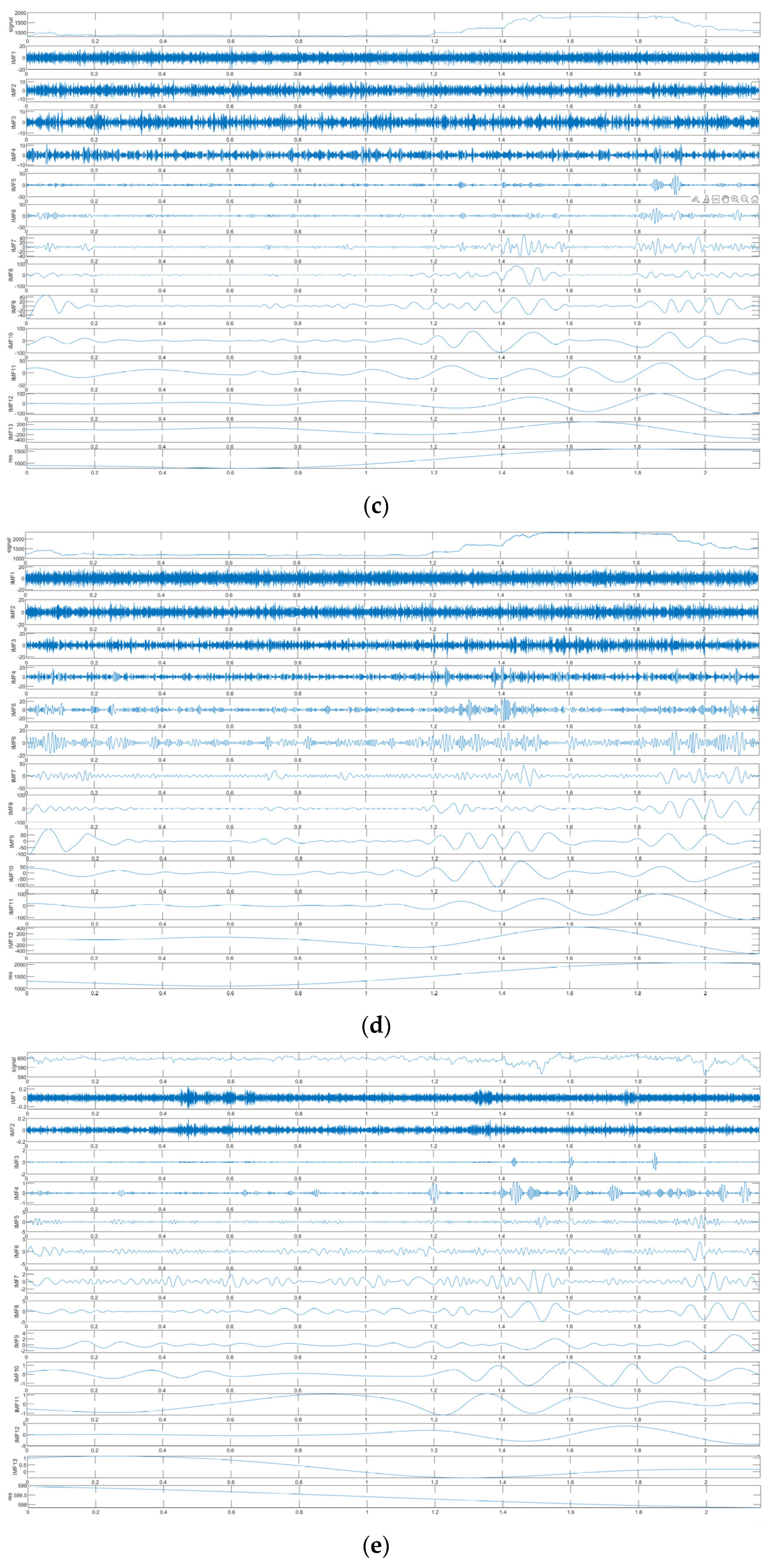
The intermediate point temperature model is affected by factors such as the unit load, the coal quantity, the main feed water flow, the total air volume, and the feed water temperature. It is a typical nonlinear and non-stationary signal. Therefore, this work proposes an EEMD–LSTM coupling model. The model decomposes the intermediate point temperature sequence into a series of IMF components using EEMD decomposition. The decomposed input sequence is shown in Figure 3a–e, and the output sequence of the output intermediate point temperature is shown in Figure 3f. The first behavior inputs the original output power of the variable, and the IMF is the decomposed sequence, the remaining component of the last behavior, which then selects the subsequences highly correlated with the target variable to input into the multi-layer LSTM network. Finally, the subsequence prediction results are reconstructed to obtain the prediction results. For the more stable second-by-second data of the operating unit on 30 July 2022, the data within each 4 s were averaged, and the temperature sequence with a resolution of 4 s was formed after preprocessing. EEMD decomposition was performed on the five input variables. Through observation, it can be seen that the fluctuation trend of the IMF component had certain similarities overall, but the details of the fluctuation were different. The IMFs and residual components of each input variable were added to other factors as the prediction conditions for the LSTM model.

The specific modeling process was as follows:

(1)

EEMD decomposition

Using the EEMD decomposition method, the signal $x\left(t\right)$ was decomposed into the IMF component and the residual component $R_n$.

(2)

IMF component extraction

Pearson correlation coefficients of the IMF component and the residual component $R_n$ and $x\left(t\right)$ were calculated, denoted as $P=\left\{p_1,p_2,\cdots ,p_n\right\}$. 1/(2(n + 1)) of Pearson’s correlation coefficient was taken as the threshold $p_0$ for the correlation coefficient, where n is the sum of the number of IMF components and the number of $R_n$ of the remaining components.

$$p_0=\frac{\sum _{i=1}^n{p}_i}{2(n+1)}$$

(6)

For any two equal length vectors X and Y, Pearson’s correlation coefficient can be expressed as [32]:

$$\begin{array}{c}{p}_{X,Y}=\frac{\mathrm{cov}(X,Y)}{{\sigma }_X{\sigma }_Y}=\frac{E\left(\left(X-{\mu }_X\right)\left(Y-{\mu }_Y\right)\right)}{{\sigma }_X{\sigma }_Y}=\\ \frac{E\left(XY\right)-E\left(X\right)E\left(Y\right)}{\sqrt{E\left(X^2\right)-E^2\left(X\right)}\sqrt{E\left(Y^2\right)-E^2\left(Y\right)}}\end{array}$$

(7)

According to Equation (5), the value range of $p_i$ is between −1 and 1, and when the absolute value of $p_i$ is close to 1, it shows a strong correlation. When the absolute value of $p_i$ approaches 0, it is said to be uncorrelated. The IMF component or $R_n$ component with high correlation can be screened out according to the threshold $p_0$.

(3)

LSTM network prediction

In order to reduce the influence caused by different dimensions of the temperature series after decomposition, the selected components with high correlation are normalized [33]. After being input to the LSTM neural network, the prediction result of the subsequence is obtained. The sub-temperature prediction components are reverse normalized and then superimposed to obtain the final intermediate temperature prediction results. Initial parameter settings: the maximum number of training times was set to 20, the Minibatch Size was selected as 128, the initial learning rate was 0.01, the learning rate was adjusted to 70 after training, the learning rate adjustment factor was 0.2, there were two neural network layers, there were two fully connected layers, the input dimensions were set to five, the output dimensions were set to one, and the mean absolute error function was selected as the loss function, Adam as the optimization function, and tanh as the activation function. Due to the large amount of data, in order to alleviate the overfitting phenomenon, the Dropout was set to 0.2, of which 70% of the sample data were used as the training set, and 30% of the sample data were used as the testing set. The IMF components obtained from the EEMD decomposition were input into the LSTM model for training, and the resulting optimal adaptation parameters were set as follows: the maximum training times were set to 20, the Minibatch Size was selected as 64, the initial learning rate was 0.01, the adjusted learning rate after training was 70, and the learning rate adjustment factor was 0.2. There were two neural network layers, there were two fully connected layers, the input dimension was set to five, and the output dimension was one. The average absolute error function was selected as the loss function, with Adam as the optimization function and tanh as the activation function. Due to the large amount of data, the Dropout was set to 0.2 to mitigate overfitting. Finally, 70% of the sample data were used as the training set, and 30% of the sample data were used as the testing set.

The evaluation indexes of the experimental results are as follows:

MAE (mean absolute error) is the mean absolute error, and its calculation formula is:

$$X_{MAE}=\frac{1}{n}{\sum }_{t=1}^n\left|y_t-\widehat{y_t}\right|$$

(8)

RMSE (root mean square error) is the root mean square error, and its calculation formula is:

$$X_{\mathrm{RMSE}}=\sqrt{\frac{1}{n}{\sum }_{i=1}^n{\left(y_i-{\widehat{y}}_i\right)}^2}$$

(9)

MAPE (mean absolute percentage error) is the mean absolute percentage error, and its calculation formula is:

$$X_{\mathrm{MAPE}}=\frac{1}{n}{\sum }_{i=1}^n\frac{\left|y_i-{\widehat{y}}_i\right|}{y_i}$$

(10)

The coefficient of determination R² represents the fitting effect of each model:

$$R^2=1-{\sum }_{i=1}^n{\left({\widehat{y}}_i-y_i\right)}^2/{\sum }_{i=1}^n{\left({\overline{y}}_i-y_i\right)}^2$$

(11)

In the formula:

${\widehat{y}}_i$—the ith intermediate point temperature real data;

$y_i$—the ith intermediate point temperature predicted value;

${{\overline{y}}_i}_i$—the mean of true value;

$n$—the total number of intermediate temperature data points.

4. Example Analysis of Unit Temperature Prediction Based on the EEMD–LSTM Neural Network

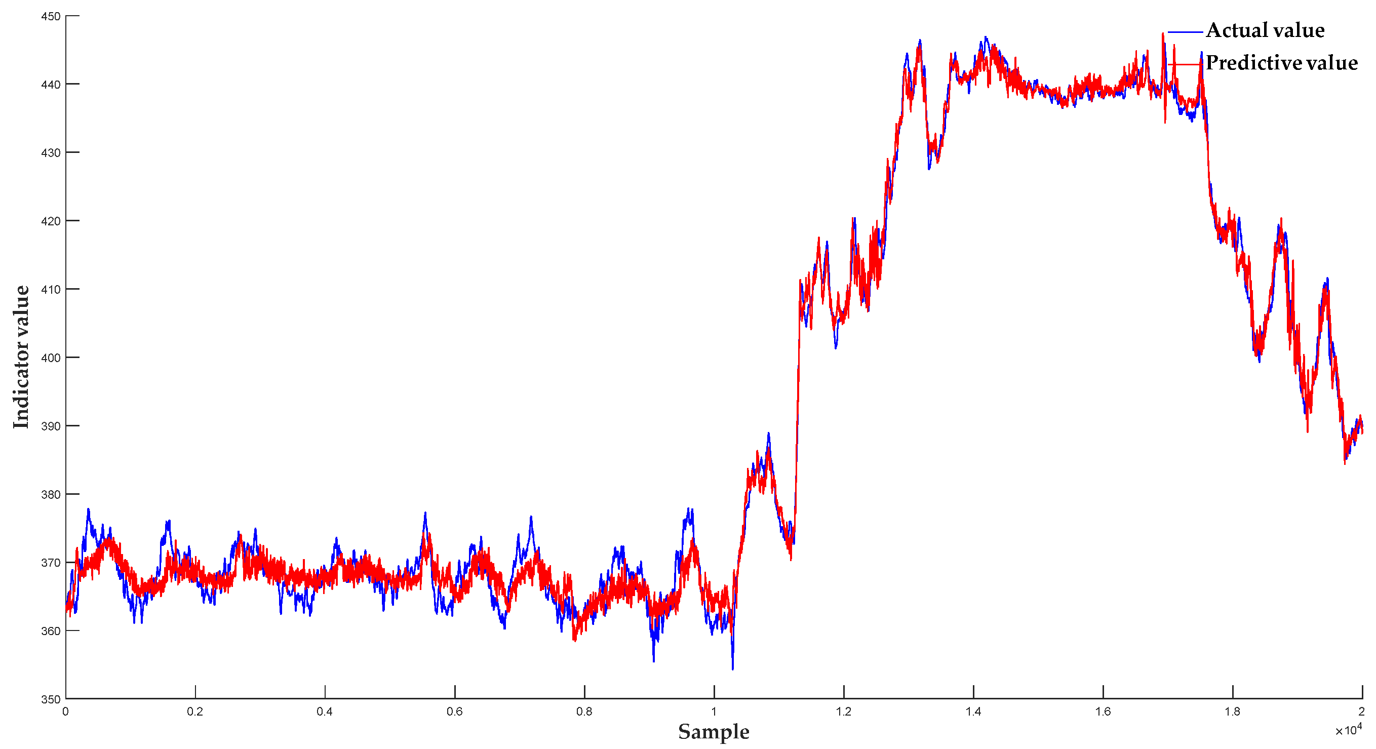
The time series data column of the intermediate point temperature was selected as the research object, and the prediction model constructed by LSTM, BP, and EEMD–LSTM, respectively, was used for short-term prediction research. The prediction results were comprehensively evaluated using four evaluation indexes: the root mean square error RMSE, the mean absolute percentage error MAPE, the determination coefficient R², and the mean absolute error MAE. We determined which of the three prediction models, BP, LSTM, and EEMD–LSTM, was superior in the prediction of intermediate point temperature time series, analyzed whether the signal decomposition technology EEMD improved the prediction accuracy, and focused on the performance of the combined model based on long-term and short-term memory neural network in the short-term prediction of the intermediate point temperature time series. This experiment was implemented on the MATLAB 9.9.0.1467703 (R2020b) software platform.

In this work, the operation data of all thermal power units from 16 July 2022 to 2 August 2022 were analyzed in detail, and it was found that the data on 30 July 2022 were more suitable, the unit load was more typical, the quantity of coal used was of good quality, the feedwater quantity was appropriate, and the sampling time was appropriately 4 s. Therefore, the validity of the model was verified using the operation data of a thermal power unit on 30 July 2022. The data came from the same unit. The data group was taken from the intermediate point temperature control system during the operation of a 600 MW supercritical unit, including real-time data such as the fuel quantity, feed water quantity, and intermediate point temperature, with a total of 21,600 groups, and the sampling time was 4 s. The first 15,120 groups were taken as training samples, and the last 6480 groups were taken as testing samples. We selected the following time period (00:00 to 23:56) for prediction. Analyzing the RMSE, MAE, MAPE, and R² separately, it was determined that the error of the proposed EEMD–LSTM prediction model was generally lower than that of a single prediction model. Compared with the single prediction model, the proposed EEMD–LSTM prediction model was closer to the actual temperature curve, and the fitting effect was the best.

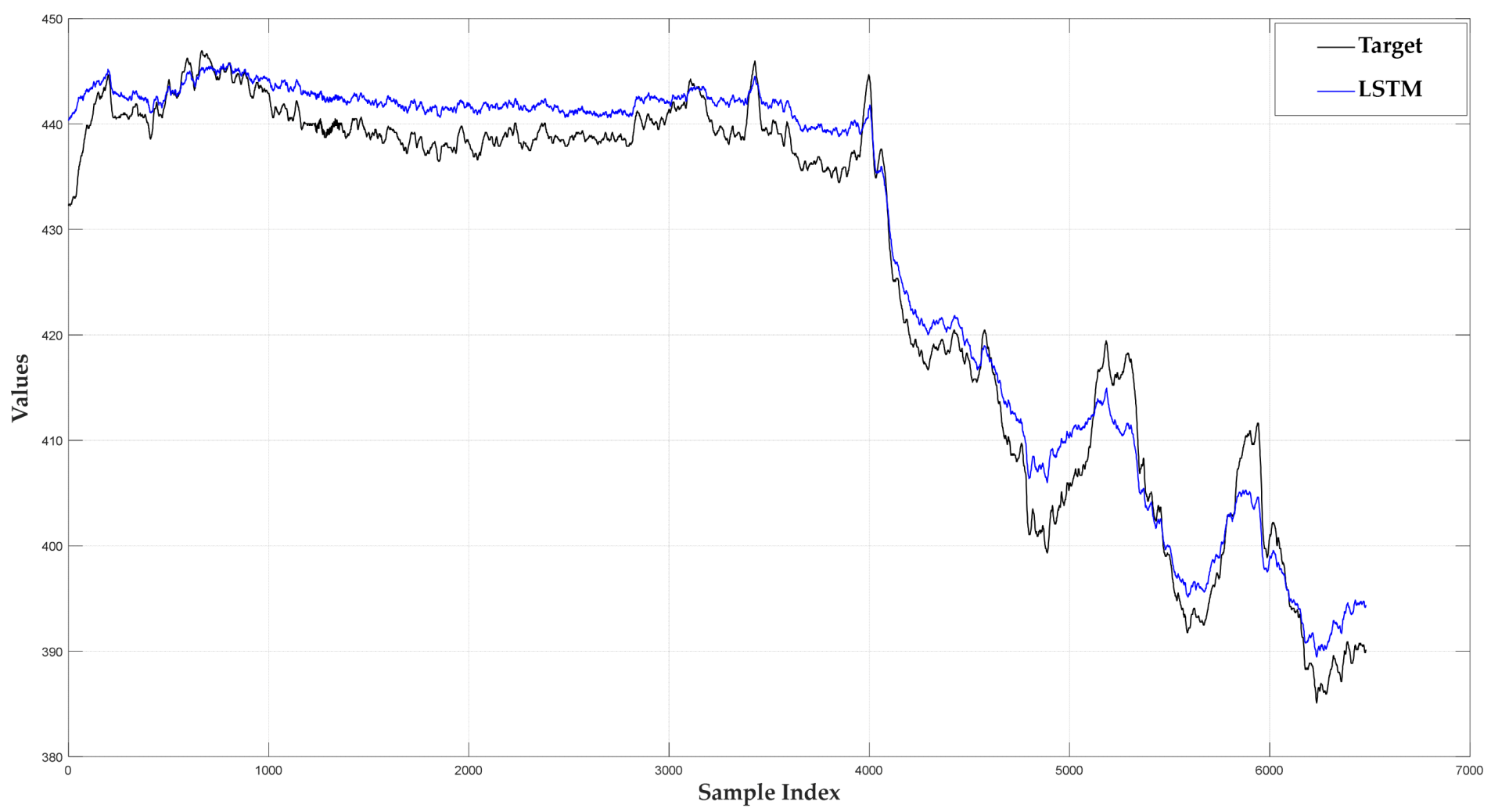
The EEMD method was used to effectively decompose the intermediate point temperature time series, input each component of the decomposition into the LSTM model for prediction, and combine and reconstruct the predicted data of all components, to obtain the prediction results of the EEMD–LSTM model. In order to verify the prediction performance and reliability of the established EEMD–LSTM model, the BP and LSTM neural network models were used to predict the time series of the intermediate point temperature. 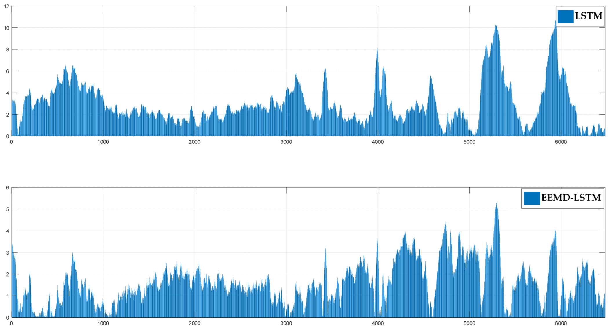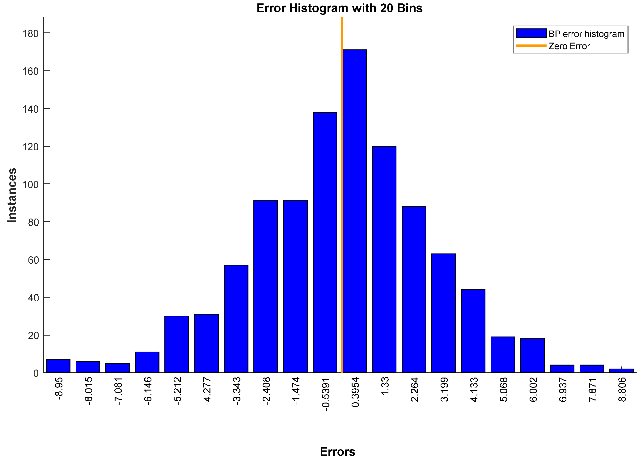The results obtained are shown in Figure 4, Figure 5 and Figure 6 below, and Figure 7 and Figure 8 show the errors of the three prediction methods.

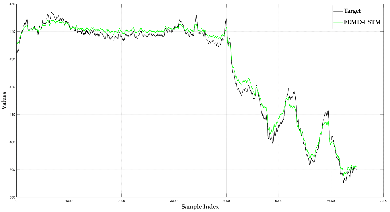
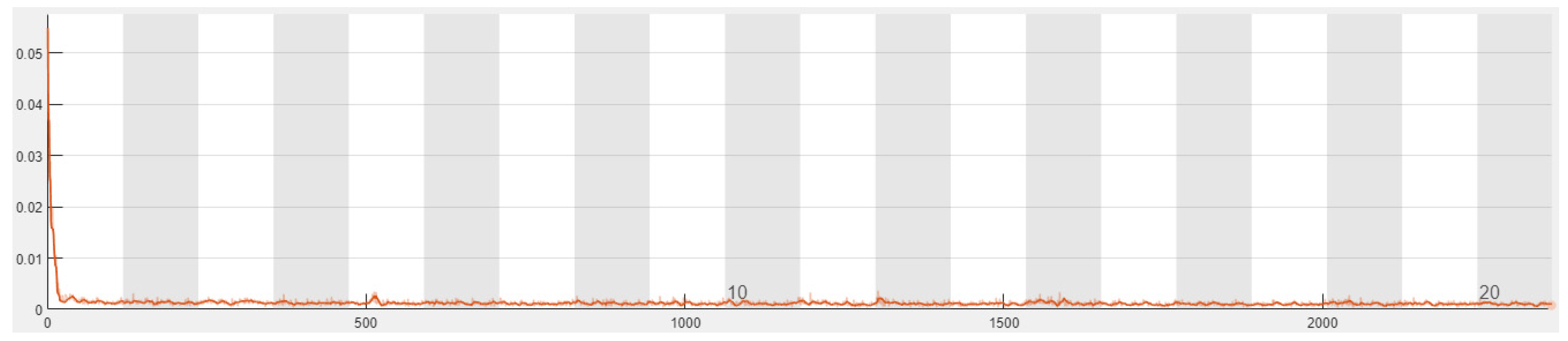
It can be seen from Figure 6 that the relative error of the prediction results of the EEMD–LSTM model was relatively stable, and the fluctuation in the relative error of the prediction results of the other two models was more prominent. It can be seen from Figure 9 that when the number of iterations was one, the model loss function value was 0.0432. When the number of iterations was 500, the model loss function value was 0.0021. As the number of iterations increased to 2000, the model error was 0.0023. Overall, the relative error of the EEMD–LSTM model was significantly smaller than that of the BP and LSTM models, and the relative error of the LSTM model in each year was smaller than that of the BP model. The results obtained from the evaluation index are shown in

Table 2. Prediction model testing set simulation results.

Model	RMSE	MAE	MAPE	R2
EEMD–LSTM	1.8849	1.6119	0.37372%	0.98891
LSTM	3.5503	2.9562	0.693%	0.96065
BP	2.8483	2.1633	0.56297%	0.99561

and

Table 3. Prediction model training set simulation results.

Model	RMSE	MAE	MAPE	R2
EEMD–LSTM	1.6905	1.1831	0.27571%	0.99108
LSTM	2.5579	2.1698	0.50393%	0.97958
BP	2.7977	2.1388	0.55712%	0.99586

. The average absolute error (MAE) and root mean square error (RMSE) of the common evaluation indexes were used. The specific calculation results of the three models are shown in Table 2 and Table 3.

Table 3 shows that the mean absolute error MAE and root mean square error RMSE of the EEMD–LSTM model prediction results were 1.1381 and 1.6905, respectively. Considering the mean absolute error MAE, the prediction performance of the EEMD–LSTM model was improved by 98.67% and 95.57%, respectively, compared with the LSTM neural network and the BP neural network. Similarly, in terms of the mean square error RMSE, the prediction performance of the EEMD–LSTM model was 86.74% and 110.72% higher than that of the LSTM neural network and the BP neural network, respectively. It can be concluded that the accuracy of the prediction results of the EEMD–LSTM model is significantly better than that of the other two models, which is mainly due to the fact that the EEMD transforms the non-stationary intermediate point temperature time series into several components with different variation rules. The predicted values of each component are more accurate after reconstruction, which effectively reduces the prediction error.

5. Conclusions

In this study, an intermediate point temperature prediction model based on the EEMD–LSTM method is proposed. This model directly performs EEMD modal decomposition on the output data to determine the local characteristics of the data for prediction. Two single models are established and compared with the proposed model. The MAPE, RMSE, MAE, and R2 are used to evaluate the prediction error. The main results are as follows: (1) The EEMD modal decomposition method is used to decompose the curve data of each input variable and to improve the progress of the LSTM prediction algorithm by extracting the curve detail components and presenting the local features of the curve in a complete way. The EEMD–LSTM model’s accuracy, compared with the LSTM model, using the root mean square error (RMSE) and the average absolute error (MAE), is increased by 86.74% and 98.67%, respectively; compared with the BP model, the accuracy was increased by 110.72% and 95.57%, respectively. Obviously, the prediction results of the EEMD–LSTM are more accurate, and the LSTM model and BP model are not as effective as the EEMD–LSTM in terms of the RMSE and MAE. (2) The prediction results show that the intermediate point temperature prediction model based on EEMD–LSTM has the characteristics of timeliness and high efficiency and can accurately predict the change in the intermediate point temperature. The obtained model can objectively reflect the dynamic change law of the intermediate point temperature and has good prediction accuracy and generalization ability, which confirms the feasibility of the method. At the same time, it is pointed out that the EEMD–LSTM neural network automatically determines the network structure and model parameters in a self-organizing manner, without too much experience and artificial adjustment; hence, it has more practical significance and application value. (3) The results show that the relative error of the EEMD–LSTM model prediction results is relatively stable and significantly smaller than those of the BP and LSTM neural network models. Compared with the other two models, the EEMD–LSTM model can predict the intermediate point temperature more accurately. There are few studies for prediction based on the combined model of EEMD and LSTM in this field. The EEMD–LSTM prediction model established in this work has certain application value in the field of intermediate point temperature prediction and can meet the requirements of the short-term prediction of the intermediate point temperature. In theory, the neural network has strong adaptive characteristics and online training ability, but in practical applications, it still has its own shortcomings that are difficult to overcome. For example, the BP network has the problem of a slow training speed. When the system is more complex, the training time of the network is obviously longer, which limits its real-time application. In addition, in some links, there is still a lack of complete theoretical guidance, such as the number of hidden layer nodes in the network. Therefore, the present model needs algorithmic improvement to overcome the above drawbacks when used for the prediction of 1000 MW ultra-supercritical units.