Article

Transmission Line Icing Prediction Based on Dynamic Time Warping and Conductor Operating Parameters

1
College of Civil Engineering and Architecture, China Three Gorges University, Yichang 443002, China
2
College of Electrical Engineering and New Energy, China Three Gorges University, Yichang 443002, China
*
Author to whom correspondence should be addressed.
Energies 2024, 17(4), 945; https://doi.org/10.3390/en17040945
Submission received: 14 December 2023 / Revised: 27 January 2024 / Accepted: 12 February 2024 / Published: 18 February 2024
(This article belongs to the Section F5: Artificial Intelligence and Smart Energy)

Abstract

:
Aiming to improve on the low accuracy of current transmission line icing prediction models and ignoring the objective law of icing of transmission lines, a transmission line icing prediction model considering the effect of transmission line tension on the bundle of icing thickness is proposed, based on a convolutional neural network (CNN) and bidirectional gated recurrent unit (BiGRU). Firstly, the finite element calculation model of the conductor and insulator system was established, and the change rule between transmission line tension and icing thickness was studied. Then, the convolutional neural network and bidirectional gated recurrent unit were used to construct a transmission line icing thickness prediction model The model incorporated a weighted fusion of soft−dynamic time warping (Soft−DTW) and the icing change rule as the loss function. Optimal weights were determined through the utilization of the grid search algorithm and cross−validation, contributing to an enhancement of the model’s generalization capabilities and a reduction in prediction errors. The results indicate that the proposed prediction model can consider the impact of line operating parameters, avoiding the shortcomings of prediction results conflicting with actual physical laws. Compared with traditional non−mechanical models, the proposed model showed reductions in root mean square error (RMSE), mean absolute error (MAE), and mean absolute percentage error (MAPE) by 0.26–0.51%, 0.24–0.44%, and 5.77–13.33%, respectively, while the coefficient of determination (R2) increased by 0.07–0.13.

1. Introduction

China is one of the countries most severely affected by icing disasters worldwide. Severe icing has the potential to cause electrical accidents on transmission lines, such as line overload, insulator string icing flashovers, and conductor galloping [1]. For instance, in 2018, a widespread occurrence of freezing rain and snow hit the central and eastern regions of China, resulting in power outages for 1243 lines with a voltage of 10 kV or above, and affecting 2.2041 million users. Therefore, establishing a high−precision prediction model for transmission line icing holds significant practical significance for enhancing the operational maintenance and warning capabilities of these lines.
Researchers have extensively explored prediction models for transmission line icing. Icing models are mainly divided into mathematical models, based on physical mechanisms, such as the Goodwin model, Chaine model, and Makkonen model [2,3,4], and statistical models, based on simulations of measured data [5,6,7]. To develop prediction models of transmission line icing, scholars have conducted extensive research. With the development of artificial intelligence technologies, neural network methods have gradually been applied to research on the predictions of transmission line icing. In contrast to mechanistic and statistical models, neural networks have a strong solving ability for the nonlinear characteristics of icing, and high prediction accuracy. Wang feng et al. [8] combined the whale algorithm and genetic algorithm to optimize a generalized regression neural network (GRNN) to construct a cable icing prediction model; Xiong Wei et al. [9] proposed a combined RF−APJA−MKRVM prediction model considering the accumulation process of icing; Tang Wei et al. [10] used principal component analysis (PCA) to extract the main features affecting line icing, followed by particle swarm optimization (PSO) to optimize the support vector regression (SVR) to construct the icing prediction model; Xuejun Li et al. [11] proposed a probabilistic prediction model for transmission line icing thickness based on the hidden Markov model based on transmission line historical icing data; Zhang Ruizhe et al. [12] used the Pearson correlation coefficient and grey system correlation analysis method to determine environmental factors with a higher degree of correlation with the thickness of the icing, and constructed an icing prediction model based on limit random tree−grey system with multiple environmental characteristics; Li Xianchu et al. [13] proposed an artificial intelligence icing thickness prediction model based on the adaptive particle swarm optimization (AMPSO) optimized backpropagation neural network (BPNN) by selecting measurable engineering meteorological parameters as the icing influencing factors based on the icing growth process; Luo Cong et al. [14] used variational mode decomposition (VMD) to decompose the icing historical data and established an improved grey wolf optimizer (IGWO) to optimize the least squares support vector machine (LSSVM) model to predict the components; Li et al. [15] used ensemble empirical modal decomposition to adaptively decompose the icing sequence data, and constructed prediction models based on the component properties. The aforementioned neural network prediction models were all constructed following “data−driven” concepts. Although they can map the changes between micro−meteorological factors and icing thickness, they lack considerations of change rules of icing and a priori knowledge, which result in the model prediction results not matching the actual icing change rules, and there are problems of poor interpretation and poor stability [16].
In recent years, incorporating physical laws and prior knowledge into neural network models has become one of the hot topics in the field of machine learning. The most commonly used strategies are as follows:
  • Model loss function design guided by physical laws [17], where penalty terms are added to the neural network based on the laws of physical change, is a strategy that applies to most neural networks due to its low−coupling properties and is easy to understand;
  • Physical law−guided initialization strategy [18], which uses simulation data generated by mechanistic prediction models for neural network pre−training, is a strategy that can solve the problem of sparse observations; however, generating simulation data with the use of mechanistic models requires the empirical determination of model parameters.
Therefore, this study proposes a prediction model based on the strategy of model loss function design and guided by physical laws. Firstly, a finite element computational model of the conductor and insulator system was established to study the physical change law between the tension value of the transmission conductor and the icing thickness. Secondly, the hybrid convolutional neural network (CNN) and bidirectional gate recurrent unit (BiGRU) model was constructed, and the weighted fusion of microscopic soft−dynamic time warping (Soft−DTW) and the physical change law was used as the loss function of the hybrid model. In summary, a prediction model of transmission line icing based on soft−dynamic time warping and conductor operating parameters is proposed; the model was validated using data provided by the observation station, and the research results improve the theoretical basis for the anti−icing and disaster prevention of transmission lines.

2. Materials and Methods

2.1. Finite Element Model Establishment and Physical Law Analysis

The tension of the transmission line can be the most intuitive response to the icing thickness. However, as the data provided by observation stations lack tension values and include only micro−meteorological data and ice thickness, a finite element model of the transmission line–insulator system was established. Based on the provided wind speed values and ice thickness, the model simulated loads and calculated the tension of the conductor through simulation.

2.1.1. Establishment of Finite Element Model

Using ANSYS software (https://www.ansys.com/, accessed on 13 December 2023), a finite element model of the transmission line–insulator system was constructed based on the observed transmission line at the observation station, considering the actual line spacing, insulator string length, and other parameters, as shown in Figure 1. The transmission conductor utilized was JL/GIA−400/50 steel−cored aluminum stranded wire, and the insulator model was the 14*XWP−300. The physical parameters of the conductor and insulator are detailed in Table 1.
In the modeling process, the top of the insulator string was set as a fixed point where it connected to the transmission tower, as the transmission tower had little influence on the variation in the transmission line tension value. Considering that the conductor needs to be subjected to axial tension or pressure, a LINK10 rod element was used for the simulation, and the unit parameters were set to match the line characteristics [19]. The insulator string was conventionally modeled as an entire straight rod, and in order to make it closer to the actual force situation, 14 insulators were modeled using LINK8 cells and connected in an articulated manner [20].

2.1.2. Icing and Wind Load Simulation

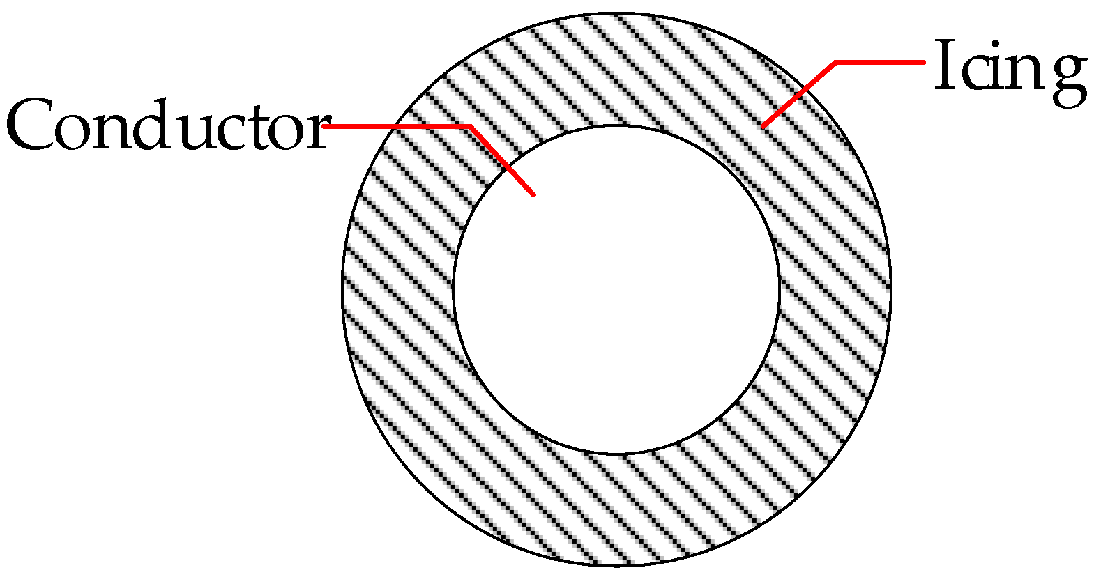
The tension in transmission lines is primarily determined by factors such as the weight of ice accumulation, conductor weight, and wind speed. The weight of the conductor was considered in the modeling process, so it was only necessary to translate the ice thickness and wind speed into loads applied to the conductor. Due to the complexity and diversity of icing on the transmission line, this study regarded icing on the transmission line as a uniform distribution of equal thickness of the icing along the conductor (as shown in Figure 2 of the cross−section of the conductor), in which the thickness of the icing was the thickness of the ice observed at the observation station.
To obtain the icing load, the volume of icing per unit length was converted into the weight of icing using a conversion formula. Subsequently, the overall icing load on the conductor was calculated. The formula for computing the icing load is expressed as follows:
F = [ π ( d + b ) 2 + π d 2 ] ρ g s
where d is the conductor radius, unit mm; b is the radius of the ice, unit mm; ρ is the density of ice, unit kg/m3; g is the acceleration of gravity, unit m/s2; and s is the conductor line length, unit m.
Wind speed is usually approximated as the sum of the average wind speed and fluctuating wind speed. Mean wind speed is typically treated as a constant, while fluctuating wind speed is simulated by a harmonic superposition method. In predictive models, wind speed is typically regarded as a scalar input feature; thus, it is processed accordingly in wind speed simulations, being considered as the mean wind speed. The wind loads acting on conductors and insulators were computed according to the specifications [21]. The formulas for calculating wind loads on conductors and insulators are shown in Equations (2) and (3).
W X = β C α L W 0 μ Z μ S C d L P B 1 sin 2 θ
W 1 = n λ 1 W 0 μ Z μ S 1 B 3 A 1
where W X is the conductor wind load; β C is the wind gust coefficient; α L is the span reduction coefficient; W 0 is the reference wind pressure; μ Z is the variation coefficient of wind pressure height; μ S C is the conductor shape coefficient; d is the outer diameter of the conductor when icing; L P is the horizontal span; B 1 is the wind load increase coefficient of conductor icing; θ is the angle between the wind direction and the wire; W 1 is the wind load of insulator; n is the number of insulators; λ 1 is the reduction coefficient; μ S 1 is the shape coefficient of insulator; B 3 is the wind load increase coefficient of insulator icing; and A 1 is the windward area of the insulator.

2.1.3. Analysis of Physical Laws

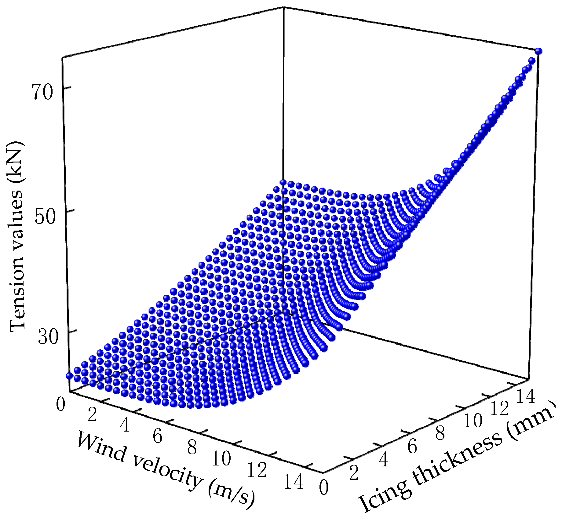
Based on the aforementioned finite element model and load simulations, the tension value of the transmission conductor was simulated under the influence of 0–15 m/s wind speed and 0–15 mm icing thickness, as shown in Figure 3. Origin software (https://www.originlab.com/origin, accessed on 13 December 2023) was used to fit wind speed, icing thickness, and tension values, with the following fitting equation:
z = a + b x + c y + d y 2 + e y 2 1 + f x + g x 2 + h x 3 + i y + j y 2
where a , b , c , d , e , f , g , h , i , j are the numerical values; x is the wind speed, unit m/s; y is the thickness of icing, unit mm; and z is the tension value, unit kN.
From Figure 3 and Equation (4), the following points can be observed:
  • When the wind speed remains constant, an increase in icing thickness leads to a corresponding increase in tension values;
  • When the icing thickness remains constant, higher wind speeds result in greater tension values.
The above law reflects the monotonous relationship between the wire tension value and the icing thickness. Based on the observation data provided by the observation station, the calculated Pearson correlation coefficient between the icing thickness and the tension values was 0.88. This suggests a positive correlation between tension values and icing thickness, which is consistent with the aforementioned physical principles. This study did not consider the physical law between micro−meteorology and icing thickness because icing thickness is affected by many factors such as wind speed, humidity, temperature, precipitation, etc., and the meteorological complexity and variability in the actual environment; therefore, it is not possible to adequately explore the law between micrometeorology and icing thickness.

2.2. Prediction Model Construction

2.2.1. Construction of the CNN−BiGRU Model

CNN are deep feedforward neural networks with characteristics such as local connectivity and weight sharing, enabling efficient feature extraction from datasets. A typical CNN consists of convolutional layers, pooling layers, and fully connected layers. The convolutional layers perform convolutional computations using custom−sized kernels to extract features from input data. The pooling layers then reduce the dimensionality of the data obtained from the convolutional operations through operations such as max pooling or average pooling, simplifying the complexity of features and data. Finally, the fully connected layers aggregate the pooled data and produce the output.
Gated recurrent units (GRU), as a variant of long short−term memory (LSTM), are built upon the internal structure of LSTM. GRU introduce reset and update gates, which effectively alleviate the issues of gradient vanishing and exploding. They also offer faster computation speeds and help prevent overfitting problems caused by excessive sequence fitting. However, as GRUs can only utilize unidirectional information, unable to consider bidirectional information, BiGRU can be employed. By obtaining information from previous and subsequent sequences, BiGRU ensure that important features are preserved to the maximum extent.
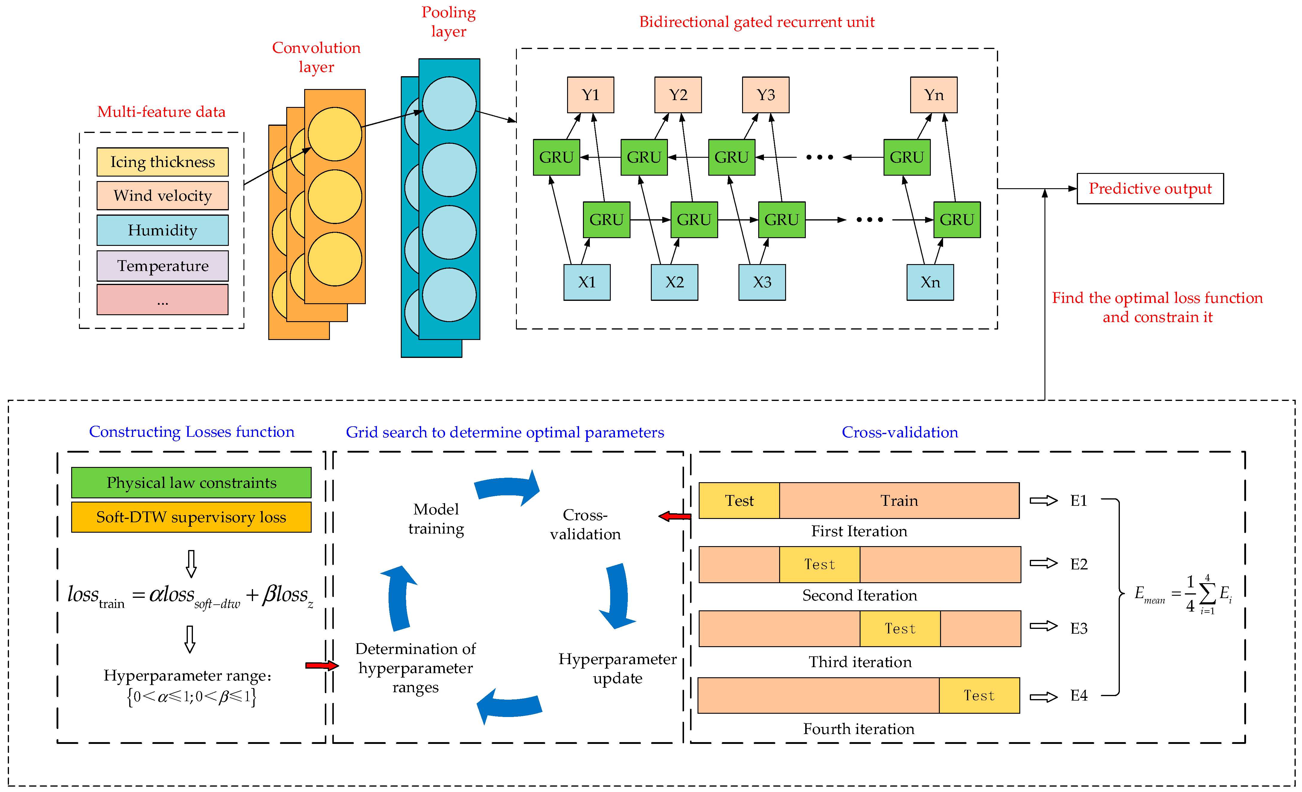
CNN, with their unique architecture, efficiently explore the inter−relationships within a multi−feature dataset using convolutional layers. By constructing temporal feature vectors through pooling layers, these vectors are input into the bidirectional gated recurrent unit (BiGRU) layer. Leveraging this network characteristic, the model can effectively learn both the past and future information of ice accumulation sequences. The structure of the CNN−BiGRU network is illustrated in Figure 4.

2.2.2. Physical Law Constraint Modeling

In this study, physical law constraints were constructed in the loss function based on the CNN−BiGRU model to measure the inconsistency of the model’s predictions with the physical laws while considering the prediction accuracy. The loss function, taking physical law constraints into account, is shown below:
l o s s train = α l o s s model + β l o s s phy
where l o s s train is the total loss function; l o s s model is the supervisory loss, which measures the difference between the actual and predicted values; α is a weighting parameter to weigh the supervisory loss; l o s s phy is the loss of physical law constraints; and β is a weighting parameter to weigh the physical law constraints.
Building upon the analysis of physical laws in Section 2.1.3 and addressing the limitations of traditional supervised losses, the following constraints are formulated.
(1) Physical law constraints on tension and icing thickness: the values of tension and icing thickness at different moments are related to each other through the following equation:
y ^ t + d y t > 0 , i f   z t + d > z t
where y ^ t + d is the predicted value of the icing thickness at moment t + d ; y t is the observed value of the icing thickness at moment t ; z t + d is the observed value of the tension value at moment t + d ; and z t is the observed value of the tension value at moment t .
To ensure that this equation can be supported in the prediction model, a loss function based on tension and icing thickness was constructed, as shown in Equation (7). A negative value of Δ [ y i , z ] in Equation (7) was considered to be a violation of the laws of physics, and was corrected by adding a Relu function to prevent such problems.
{ Δ [ y i , z ] = ( y ^ t + d y t ) ( z t + d z t ) l o s s z = 1 n i = 1 n R e l u ( Δ [ y i , z ] )
where n is the length of the time series.
(2) Constraints based on dynamic time warping: in the training process of traditional neural network models, the majority use the mean square error (MSE) or its variant (MAE) as the loss function, and then for the more volatile data such as the icing, the MSE cannot capture the sudden change in the icing in a timely manner, which results in the prediction value being slightly delayed or not conforming to the trend fluctuation. Therefore, DTW [22] can be introduced to replace MSE as a new supervised loss. DTW calculates the similarity between two different time series using a kind of warping, which telescopes the time series to obtain the optimal path between the two sequences.
For example, the measured icing thickness data A = { a 1 , a 2 , , a n } , the predicted data B = { b 1 , b 2 , , b m } , and the two time series form the path matrix C :
{ C = [ c ( a n , b 1 ) c ( a n , b 2 ) c ( a n , b m ) c ( a 2 , b 1 ) c ( a 2 , b 2 ) c ( a 2 , b m ) c ( a 1 , b 1 ) c ( a 1 , b 2 ) c ( a 1 , b m ) ] c ( a n , b m ) = ( a n b m ) 2
where c ( a n , b m ) is the relationship between each element of the two sequences.
The goal of DTW is to find the optimal regularization distance, w = { w 1 , w 2 , , w k } , in the path matrix C , i.e., to minimize the function:
D T W ( A , B ) = R ( n , m ) = min ( i = 1 k w i )
where R ( n , m ) is the cumulative distance matrix.
The regularization path needs to satisfy the following conditions:
  • Continuity: the path must maintain continuity.
  • Monotonicity: the points along the path must increase monotonically with time.
  • Boundary conditions: the path must initiate from the lower−left corner and conclude at the upper−right corner.
The optimal regularization path that satisfies the above constraints is as follows:
R ( n , m ) = C ( n , m ) + min { R ( n 1 , m 1 ) R ( n 1 , m ) R ( n , m 1 )
where min is a discrete process. If directly integrated into a neural network, the network would be incapable of executing gradient descent, thereby preventing the update of model parameters. Therefore, Soft−DTW [23] is introduced, as shown in the following equation:
{ R n , m s o f t d t w = C ( n , n ) + min γ { R ( n 1 , m 1 ) R ( n 1 , m ) R ( n , m 1 ) min γ { a 1 , , a n } = { min i n a i γ log i = 1 n e a i / γ
Using min γ instead of min in Equation (11) changes the discrete differentiability of the DTW and defines the forward and directional propagation processes, which can be found in the literature.
Combining Equations (7) and (11), the physical law constrained loss function is constructed as shown below:
l o s s train = α l o s s s o f t d t w + β l o s s z
where l o s s s o f t d t w is the supervisory loss based on SoftDTW; α is the weight coefficient measuring the supervisory loss function of SoftDTW; and β is the weight coefficient measuring the physical law of tension value and icing thickness. The constraint process is shown in Figure 4. The optimal weight coefficients can be determined based on the grid search algorithm to search for weights to find the optimal range, followed by the use of an equal proportional k−fold cross−validation algorithm to obtain the weight hyperparameters that satisfy the physical laws and minimize the error, which is able to validate the model’s ability to generalize, and also prevents the model from overfitting [24].

2.3. Experimental Data and Experimental Settings

The experimental data in this study were selected from the icing monitoring data of an observation station in a certain region. Partial data are shown in Table 2. The dataset comprised a total of 171 data points, collected at 1 min intervals. The tension values in the table were calculated using the fitting Equation (4).
In this paper, the icing monitoring data were normalized to the interval [0,1]. The normalized data were used to construct the training and test sets according to the strategy of single−step prediction. Firstly, the step size and the number of steps to be used as the input sequence were determine. Secondly, the characteristics of each step of the data (such as ice thickness, humidity, temperature, wind speed, etc.) were determine. Finally, the dataset was divided based on the number of steps and features. The time step for the icing monitoring data was set as 2, the step features were set as 4, and the length of the output sequence is set as 1. Here, 70% of the data were selected as the training set, and 30% were in the test set. The CNN−BiGRU model was then trained with the training set to predict the icing thickness in the test set.
To validate the superiority of the proposed prediction model in this study, a comparison was conducted with various models, including LSTM, CNN, the Autoregressive Integrated Moving Average Model (ARIMA), BiGRU, and CNN−BiGRU. LSTM has two hidden layers, with 128 neurons in each layer; CNNs employ two convolutional layers with 16 and 32 neurons, respectively. The model parameters of ARIMA are set as (2, 0, 0). BiGRU has two hidden layers with 128 neurons in each layer; the parameters of the model in this study were the same as those of CNN and BiGRU. The weight of the loss function was determined by the grid search cross−validation algorithm, where α = 0.78 and β = 0.56. Each model had a batch size of 16, a learning rate of 0.001, and epochs of 200. All models used Adam optimization for gradient descent.
In this study, two sets of trials were designed for comparative analysis:
  • Comparative analysis of the prediction performance with the traditional prediction model;
  • Comparative analysis of the prediction performance of the models with different constraints of physical laws.

Evaluation Indicators

The performance of the prediction model was evaluated using the metrics of root mean square error (RMSE), mean absolute error (MAE), mean absolute percentage error (MAPE), and coefficient of determination (R2). The calculation formulas are as follows:
{ R M S E = 1 N n = 1 N ( y n - y ˜ n ) 2 M A E = 1 N n = 1 N | y n - y ˜ n | M A P E = 100 % N n = 1 N | y n - y ˜ n y n | R 2 = 1 N n ( y ˜ n y n ) 2 N n ( y ¯ n y n ) 2
where N is the quantity of time series data; y ˜ n is the predicted icing thickness; y n is the actual icing thickness; and y ¯ n is the mean icing thickness.

3. Results

3.1. Performance Comparison of Traditional Prediction Models

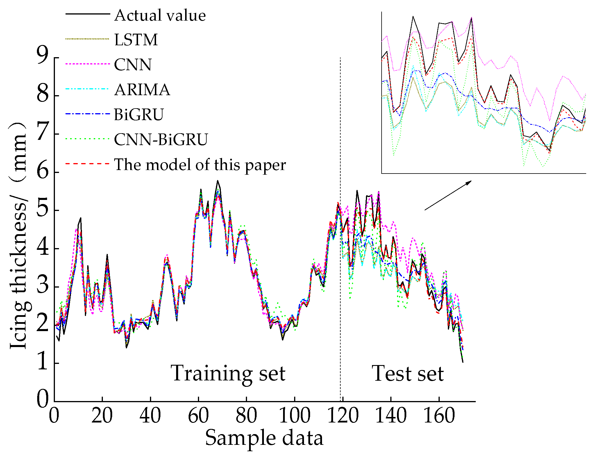
Comparative results of the prediction models proposed in this paper, and traditional models for the data provided by the observation station, are depicted in Figure 5, and the evaluation indexes of each model are shown in Table 3. It can be observed that the proposed prediction model in this paper performed the best. Compared with other prediction models, RMSE was reduced by 0.26–0.51, MAE was reduced by 0.24–0.44, MAPE was reduced by 5.77–13.33%, and R2 was increased by 0.07–0.13. Among them, the BiGRU model had better prediction accuracy than the LSTM, ARIMA, and CNN models, which verifies that its bidirectional structure and gating mechanism can effectively model the time dependence of icing changes; the prediction results of the CNN model exhibit obvious fluctuations, which indicates that its special network structure can effectively capture the features in the icing sequence. Both models indirectly demonstrated the superiority of the hybrid model, and the prediction accuracy of the CNN−BiGRU model was significantly higher than that of the traditional model. The model proposed in this paper, compared with the CNN−BiGRU model without considering physical constraints, showed a reduction of 61% in RMSE, a decrease of 67% in MAE, a decline of 58% in MAPE, and an increase of 7.78% in R2. This further emphasizes the significance and effectiveness of considering physical law constraints.
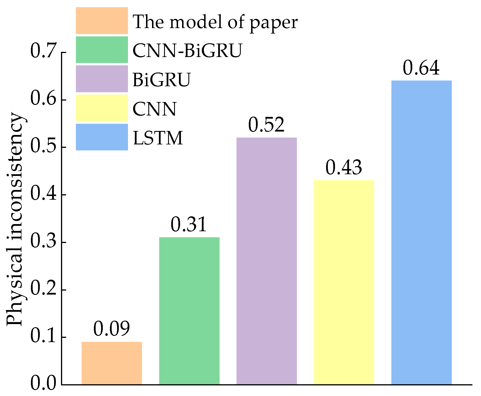
In addition to the evaluation metrics, ensuring the physical inconsistency of the model is a crucial metric in the prediction process [25], achieved by calculating the proportion of time steps for which the model makes physically inconsistent predictions (i.e., violates the physical laws presented in Equation (7)), and therefore performs a comparative analysis of the physical inconsistency based on the above model, as shown in Figure 6.
The physical inconsistency of the CNN model depicted in the figure was lower than that of other traditional models, possibly due to its unique network structure, enabling it to learn feature laws in the icing data. The prediction accuracies of CNN−BiGRU and BiGRU were greater than those of the remaining traditional models, likely because they sacrifice physical consistency to achieve a higher level of accuracy. It can be observed that the model proposed in this paper exhibited higher levels of prediction accuracy and physical consistency after considering the physical laws, further emphasizing the value of introducing physical law constraints to enhance the model’s generalization ability.

3.2. Performance Comparison of Prediction Models with Different Physical Constraints

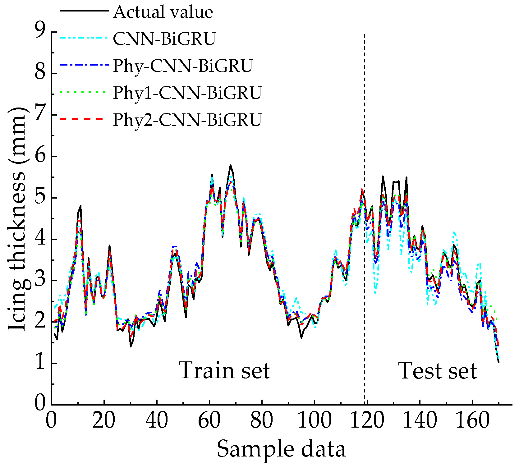
To assess the impact of different physical constraints on icing thickness predictions, the CNN−BiGRU model, Phy−CNN−BiGRU model, Phy1−CNN−BiGRU model, and Phy2−CNN−BiGRU model were used. Among them, CNN−BiGRU uses MSE supervised loss, Phy−CNN−BiGRU uses Soft−DTW + physical law constraints, Phy1−CNN−BiGRU uses MSE supervised loss + physical law constraints, and Phy2−CNN−BiGRU uses Soft−DTW supervised loss. Figure 7 and Table 4 present the prediction comparison results and evaluation indexes of the above models. The following is evident:
  • The predictive performance of CNN−BiGRU models, considering physical law constraints, surpassed that of CNN−BiGRU models, considering a single supervised loss. This suggests that physical law constraints can effectively enhance the prediction accuracy of the models;
  • The CNN−BiGRU model considering Soft−DTW outperformed the CNN−BiGRU model, considering MSE supervised loss. This suggests that Soft−DTW can better account for the similarity between predicted values and actual values, thereby enhancing prediction accuracy;
  • Phy−CNN−BiGRU outperformed other models, indicating that under the combined effect of dynamic time regularization and physical law constraints, the model more comprehensively considers the similarity between predicted and actual values and the influence of physical laws on the icing thickness; thus, the prediction results are closer to the line icing thickness.
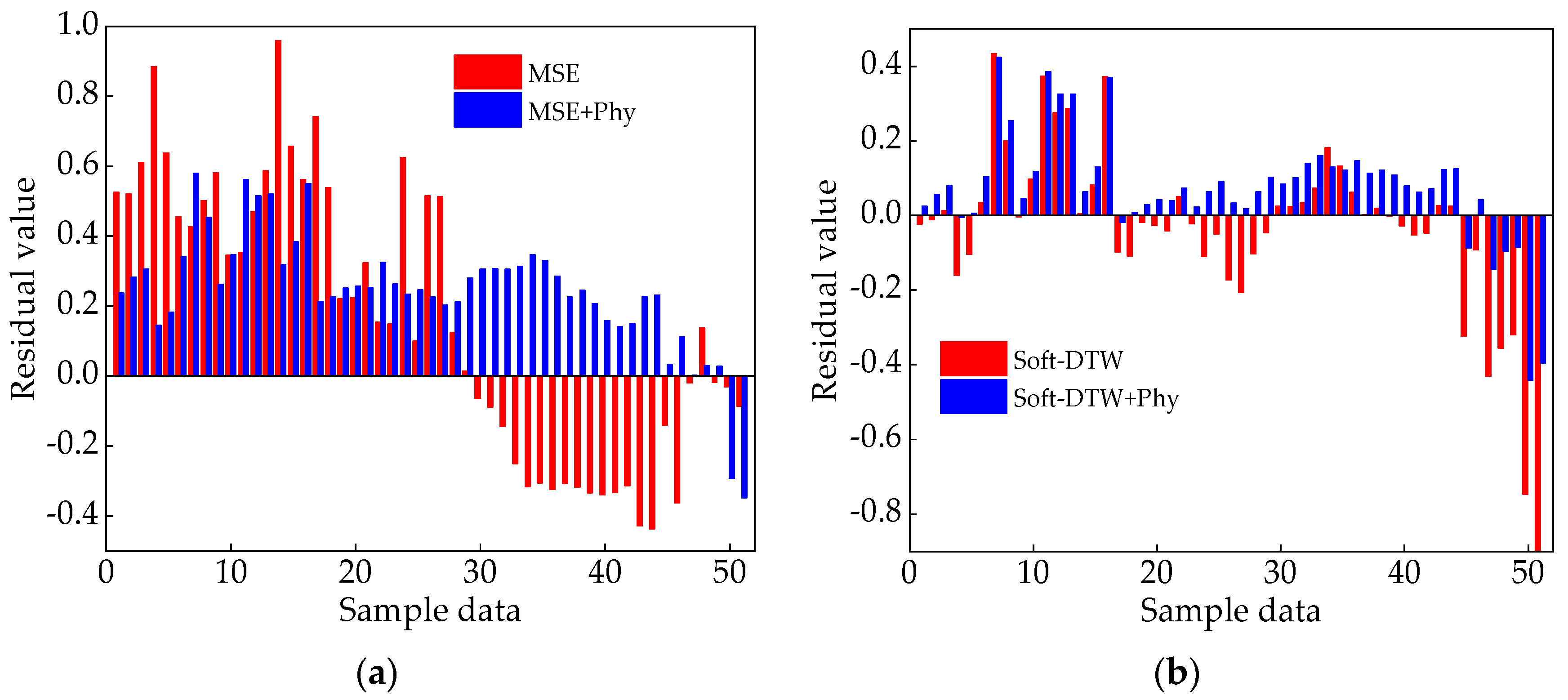
To offer a more visually compelling representation of the impact of physical law constraints on the models, a residual analysis of the test set for each model is presented in Figure 8.
Figure 8 shows that, compared with mean squared error (MSE) and Soft−DTW alone, the inclusion of physical law constraints resulted in fewer negative residual values. This suggests an effective reduction in falsely low prediction values and an improvement in the model’s reliability. Furthermore, the addition of Soft−DTW led to consistently smaller residual values compared with MSE, indicating its effectiveness in enhancing similarity between predicted and actual values. Figure 7 also indicates that the proposed model predicted the trend in icing thickness more closely to the actual values.

3.3. Sensitivity Analysis of Weight Parameters

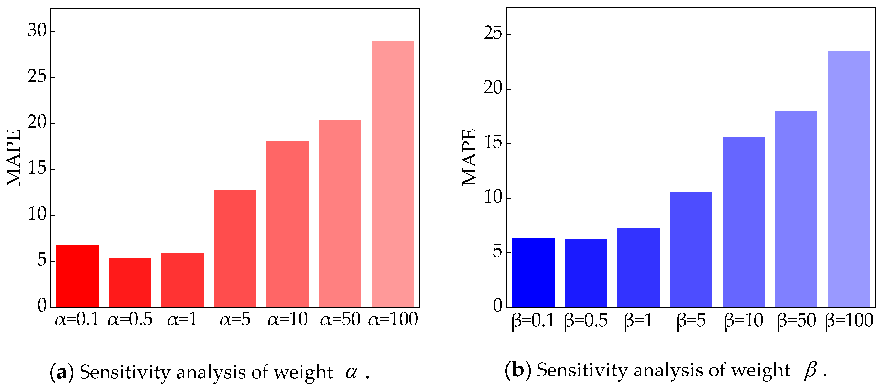
Sensitivity analyses were conducted on the weighting parameters in the loss function to verify the impact of α and β on the prediction performance. In the experiment, only the target weighting parameters were changed, and the remaining optimal parameter combinations are kept. Figure 9 presents the following observations:
  • As the weight parameters, α and β , increase in value, the model’s prediction performance deteriorates. The reason may be that the weight amplifies the penalty, exacerbating the difference between the predicted value and the measured value;
  • When the parameter weights, α and β , are between 0.1 and 1, the model has the best predictive performance;

4. Discussion

The above experimental results show that the prediction model constructed in this study effectively improves the accuracy and stability of icing thickness prediction. Compared with the traditional prediction model, RMSE is reduced by 0.26–0.51, MAE is reduced by 0.24–0.44, MAPE is reduced by 5.77–13.33%, and R2 is increased by 0.07–0.13. The main reasons are as follows:
  • The introduction of the relationship between tension values and icing thickness as the model loss function alleviates the overfitting problem in the traditional non−mechanistic models to a certain extent. Utilizing grid search and cross−validation to determine weight hyperparameters that adhere to physical laws and minimize errors enhances the model’s generalization ability, reducing the errors.
  • Soft−DTW is introduced to replace the traditional supervised loss, and the similarity of the two sets of time series data is considered during the network training process. Compared with the traditional neural network model, the sudden change in icing can be captured in time so that its prediction value is more in line with the trend fluctuation.
  • A hybrid CNN−BiGRU prediction model, incorporating micrometeorological factors, is employed to build a multi−feature dataset. This model fully leverages micro−meteorological and icing thickness feature information through the CNN. Subsequently, it utilizes the BiGRU network’s characteristics to comprehensively learn the past and future information of icing sequences, thereby enhancing prediction accuracy.
The change in icing thickness is a complex process involving multiple factors, and it is difficult to describe its change comprehensively and accurately. However, the prediction model proposed in this paper takes into account the pattern of change between the wire tension value and the icing thickness, which can be applied to the prediction of transmission line icing in most areas, because the pattern of change between the wire tension value and the icing thickness can be easily determined according to the sensors or simulation calculations, unlike the pattern of change between the micro-meteorology and the icing, which is more complicated to consider (e.g., if a loss function is built based on the pattern of change between wind speed and icing thickness, the effects of temperature, humidity and other factors on wind speed, and the meteorological complexity of each region must also be considered; therefore, the established model will not be universally applicable). Therefore, future research should explore the relationship between micro-meteorological factors and icing, integrate them into the prediction model, and establish a prediction model with universal applicability and high accuracy.

5. Conclusions

In this paper, for the problem of icing thickness prediction, an icing prediction model based on soft-dynamic time warping and conductor operating parameters is proposed. The model constructs the law of change between the value of conductor tension and the thickness of icing as the loss function of the model, realizes the constraint of considering the physical a priori knowledge in the training process of the model, and introduces Soft-DTW to replace the traditional supervisory loss in the model, which provides a new way of thinking for the construction of data-driven and knowledge-driven fusion of icing prediction models and improves the theoretical basis for the anti-icing and disaster prevention of power transmission lines.

Author Contributions

Conceptualization, F.W. and H.L.; Methodology, F.W. and H.L.; Software, H.L.; Formal analysis, H.L.; Writing, F.W. and H.L.; Visualization, Z.M.; Supervision, F.W. and Z.M. All authors have read and agreed to the published version of the manuscript.

Funding

This research was funded by National Natural Science Foundation of China (No. 51778343) and China Electric Power Engineering Consultants Group Limited Science and Technology Funding Programme (DG1-D02-2018).

Data Availability Statement

The data that support the findings of this study are available from the corresponding author upon reasonable request.

Conflicts of Interest

The authors declare no conflicts of interest.

References

  1. Guoqiang, Z.; Yue, Z.; Ying, Y.; Lei, Y.; Zhihui, W.; Yong, L. Galloping Characteristics of 10 kV Overhead Distribution Lines in Strong Wind and lcing Environment. Proc. CSU-EPSA 2022, 34, 87–92. [Google Scholar]
  2. Goodwin, E.J., III; Mozer, J.D.; Digioia, A.M., Jr.; Power, B.A. Predicting Ice and Snow Loads for Transmission Line Design. In Predicting Ice & Snow Loads for Transmission Line Design; Defense Technical Information Center: Fort Belvoir, VA, USA, 1983. [Google Scholar]
  3. Chaîné, P.; Castonguay, G. New Approach to Radial Ice Thickness Concept Applied to Bundle-like Conductors; Stanford University: Stanford, CA, USA, 1974. [Google Scholar]
  4. Makkonen, L. Models for the growth of rime, glaze, icicles and wet snow on structures. Phil. Trans. R. Soc. A 2000, 358, 2913–2939. [Google Scholar] [CrossRef]
  5. Bin, T.; Shengfeng, Z.; Tang, F.; Jun, L.; Hongliang, Z.; Xiao, Z. Research and analysis of annual failure rate of transmission line ice damag. Electr. Meas. Instrum. 2020, 57, 5. [Google Scholar]
  6. Tao, F.; Jiazheng, L.; Xunjian, X.; Li, Y.; Jun, G.; Li, L. The law of continuous ice-covering days of power grid based on freezing rain and fog observatio. High Volt. Technol. 2018, 44, 7. [Google Scholar]
  7. Jones, K.F. A simple model for freezing rain ice loads. Atmos. Res. 1998, 46, 87–97. [Google Scholar] [CrossRef]
  8. Feng, W.; Jinwei, M.; Zhangjun, L. Combined whale algorithm and genetic algorithm to optimise GRNN for prediction of icing thickness on inclined cable. J. Civ. Environ. Eng. 2022, 44, 10. [Google Scholar]
  9. Wei, X.; Hao, X.; Linxiang, X.; Kefan, Z.; Benshun, Y. A combined RF-APJA-MKRVM transmission line icing prediction model taking into account the time accumulation effect. High Volt. Technol. 2022, 48, 10. [Google Scholar]
  10. Wei, T.; Xun, S.; Jiabi, L.; Jian, W. Research on short-term icing thickness prediction model of transmission line based on optimised SVRM. J. Shaanxi Univ. Sci. Technol. 2023, 41, 151–157. [Google Scholar]
  11. Xuejun, L.; Anlong, H.; Guobin, X.; Yong, W.; Zhipeng, S.; Linhe, L. Probabilistic prediction of transmission line icing thickness based on improved hidden Markov mode. J. Xi’an Univ. Technol. 2023, 39, 586–594. [Google Scholar]
  12. Ruizhe, Z.; Kai, Z.; Liuxue, Z.; Lei, T.; Hongda, L.; Yani, W.; Yingmiao, C.; Chunshen, L.; Shuai, C. Icing prediction technology for transmission lines in Beijing based on micrometeorological microtopography. Sci. Technol. Eng. 2022, 22, 14744–14751. [Google Scholar]
  13. Xianchu, L.; Xi, Z.; Jie, L.; Jianlin, H. AMPSO-BP neural network prediction model for transmission line conductor icin. Electr. Power Constr. 2021, 42, 7. [Google Scholar]
  14. Cong, L.; Lidong, F.; Xuewen, Z.; Yuan, A. Research on icing prediction model based on VMD-IGWO-LSSVM. Grid Clean Energy 2021, 37, 9. [Google Scholar]
  15. Li, H.; Chen, Y.; Zhang, G.; Li, J.; Zhang, N.; Du, B.; Liu, H.; Xiong, N. Transmission line ice coating prediction model based on EEMD feature extraction. IEEE Access 2019, 7, 40695–40706. [Google Scholar] [CrossRef]
  16. Hunter, J.M.; Maier, H.R.; Gibbs, M.S.; Foale, E.R.; Grosvenor, N.A.; Harders, N.P.; Kikuchimiller, T.C. Framework for developing hybrid process-driven, artificial neural network and regression models for salinity prediction in river systems. Hydrol. Earth Syst. Sci. Discuss. 2018, 22, 2987–3006. [Google Scholar] [CrossRef]
  17. Jia, X.; Xie, Y.; Li, S.; Chen, S.; Zwart, J.; Sadler, J.; Appling, A.; Oliver, S.; Read, J. Physics-guided machine learning from simulation data: An application in modeling lake and river systems. In Proceedings of the 2021 IEEE International Conference on Data Mining (ICDM), Auckland, New Zealand, 7–10 December 2021; pp. 270–279. [Google Scholar]
  18. Reichstein, M.; Camps-Valls, G.; Stevens, B.; Jung, M.; Denzler, J.; Carvalhais, N.; Prabhat, f. Deep learning and process understanding for data-driven Earth system science. Nature 2019, 566, 195–204. [Google Scholar] [CrossRef] [PubMed]
  19. Zhongbin, L.; Hang, B.; Xiaohui, Y.; Wenjuan, L. Analysis of wind bias of an AC ultra-high voltage line. High Volt. Electr. Appar. 2019, 55, 170–177. [Google Scholar]
  20. Jing, M.; Jiong, C.; Xiangyi, B. Wind-bias stress analysis of disc-shaped suspended porcelain insulators under multi-rigid body model. Electr. Porcelain Surge Arrester 2021, 210–216. [Google Scholar]
  21. DL/T 5551-2018; Overhead Transmission Line Load Specificatio. National Energy Board: Beijing, China, 2018.
  22. Lichtenauer, J.F.; Hendriks, E.A.; Reinders, M.J. Sign language recognition by combining statistical DTW and independent classification. IEEE Trans. Pattern Anal. Mach. Intell. 2008, 30, 2040–2046. [Google Scholar] [CrossRef] [PubMed]
  23. Cuturi, M.; Blondel, M. Soft-dtw: A differentiable loss function for time-series. In Proceedings of the International Conference on Machine Learning, Sydney, Australia, 6–11 August 2017; pp. 894–903. [Google Scholar]
  24. Hao, C.; Zecheng, Y.; Bo, Y. Physical law-supervised interpretable machine learning method for seismic damage patterns of RC columns. J. Build. Struct. 2023, 44, 69–79. [Google Scholar]
  25. Daw, A.; Karpatne, A.; Watkins, W.D.; Read, J.S.; Kumar, V. Physics-guided neural networks (pgnn): An application in lake temperature modeling. In Knowledge Guided Machine Learning; Chapman and Hall/CRC: Boca Raton, FL, USA, 2022; pp. 353–372. [Google Scholar]
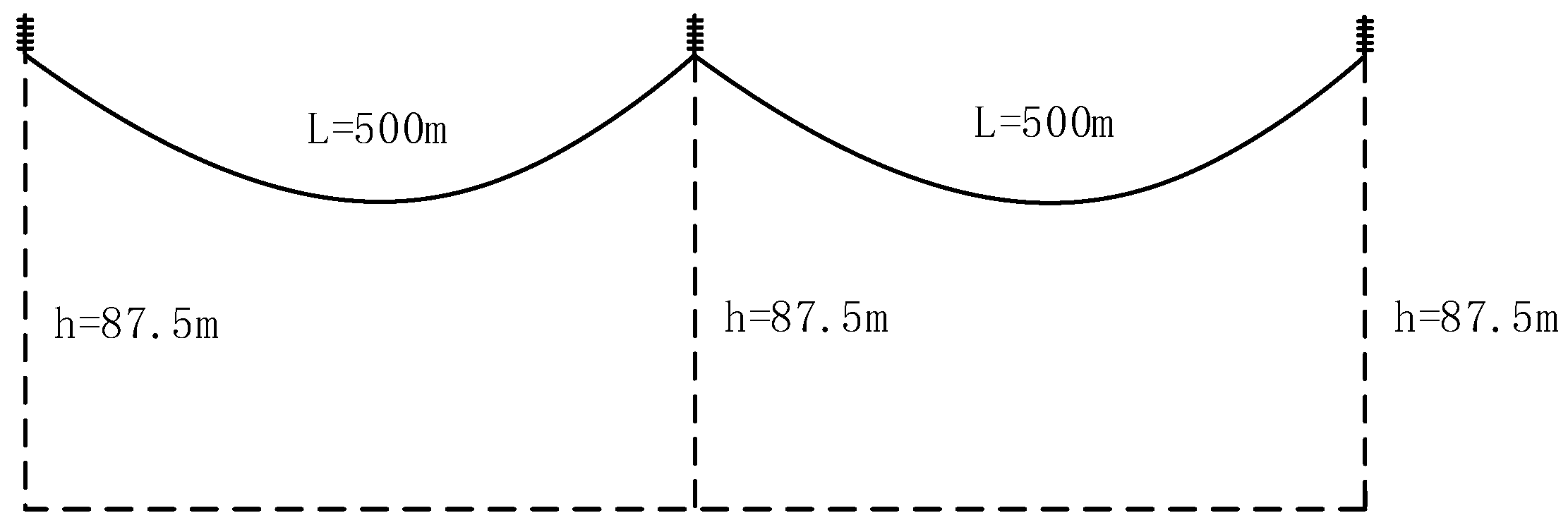
Figure 1. Line geometry diagram.
Energies 17 00945 g001
Figure 2. Uniformly icing conductor cross−sections.
Energies 17 00945 g002
Figure 3. Transmission conductor tension values.
Energies 17 00945 g003
Figure 4. Structure of the prediction model.
Energies 17 00945 g004
Figure 5. Comparison results of traditional model predictions.
Energies 17 00945 g005
Figure 6. Model physical inconsistency.
Energies 17 00945 g006
Figure 7. Prediction and comparison results of different physical constraints.
Energies 17 00945 g007
Figure 8. The above figures reflect the residual results for different physically constrained models: (a) residual analysis of the residual comparison results for CNN−BiGRU and PHY1−CNN−BiGRU; (b) residual analysis of the residual comparison results for PHY−CNN−BiGRU and PHY2−CNN−BiGRU.
Energies 17 00945 g008
Figure 9. Sensitivity analysis of the hyperparameters of physical constraint loss functions.
Energies 17 00945 g009
Table 1. Parameters of conductors and insulators.
Wire ParametersInsulator Parameters
Conductor cross−section (mm2)451.55Elastic modulus (MPa)2.8 × 10⁵
Diameter (mm)27.63Poisson ratio0.025
Weight (kg/km)1511Quality (kg)13
Elastic coefficient (N/mm2)69,000Height (m)0.195
Linear expansion coefficient (10–6/℃)19.3Face area (m2)0.03
Table 2. Icing monitoring data.
Serial NumberIcing Thickness (mm)Humidity (%)Temperature (°C)Wind Velocity (ms−1)Tension Values (n)
11.8686.97−7.764.6523,720.21
21.7186.42−7.884.1623,434.22
1701.3887.53−3.557.0119,959.8
1711.0287.88−3.637.0420,813.64
Table 3. Traditional model evaluation indicators.
Forecasting ModelRMSEMAEMAPER2
LSTM0.660.5416.02%0.84
CNN0.540.4917.41%0.85
ARIMA0.670.5617.55%0.82
BiGRU0.510.3811.14%0.88
CNN−BiGRU0.420.369.99%0.90
The model of paper0.160.124.22%0.97
Table 4. Evaluation indexes of different physical constraint models.
Forecasting ModelRMSEMAEMAPER2
CNN−BiGRU0.420.369.99%0.9026
PHY−CNN−BiGRU0.290.277.79%0.9297
PHY1−CNN−BiGRU0.230.146.34%0.9548
PHY2−CNN−BiGRU0.160.124.28%0.9769
Disclaimer/Publisher’s Note: The statements, opinions and data contained in all publications are solely those of the individual author(s) and contributor(s) and not of MDPI and/or the editor(s). MDPI and/or the editor(s) disclaim responsibility for any injury to people or property resulting from any ideas, methods, instructions or products referred to in the content.