A Trip-Based Data-Driven Model for Predicting Battery Energy Consumption of Electric City Buses

Abstract

The paper presents a novel approach for predicting battery energy consumption in electric city buses (e-buses) by means of a trip-based data-driven regression model. The model was parameterized based on the data collected by running a physical experimentally validated e-bus simulation model, and it consists of powertrain and heating, ventilation, and air conditioning (HVAC) system submodels. The main advantage of the proposed approach is its reliance on readily available trip-related data, such as travel distance, mean velocity, average passenger count, mean and standard deviation of road slope, and mean ambient temperature and solar irradiance, as opposed to the physical model, which requires high-sampling-rate driving cycle data. Additionally, the data-driven model is executed significantly faster than the physical model, thus making it suitable for large-scale city bus electrification planning or online energy consumption prediction applications. The data-driven model development began with applying feature selection techniques to identify the most relevant set of model inputs. Machine learning methods were then employed to achieve a model that effectively balances accuracy, simplicity, and interpretability. The validation results of the final eight-input quadratic-form e-bus model demonstrated its high precision and generalization, which was reflected in the R² value of 0.981 when tested on unseen data. Owing to the trip-based, mean-value formulation, the model executed six orders of magnitude faster than the physical model.

1. Introduction

The transition to electric urban bus transportation is recognized as a vital strategy for cutting pollutant and greenhouse gas emissions, reducing noise pollution, and increasing passenger satisfaction [1]. On the other hand, this transition faces significant challenges, including increased investment costs related to fully electric buses (e-buses) and their charging infrastructure, as well as operational constraints corresponding to limited vehicle range and extended charging durations in comparison to conventional buses [2]. Systematic planning of the city bus electrification process is an essential step towards the reduction of both capital and operational expenditures and mitigating the operational constraints [3].

Various factors such as traffic congestion, road gradients, passenger load (ridership), and ambient conditions (temperature, solar irradiance) can significantly influence e-bus energy consumption [4]. Thus, predicting e-bus battery energy consumption by means of a mathematical model becomes a pivotal point for transport planners and operators in their effort to optimize the transport system electrification process [5]. This process includes e-bus scheduling [6] and/or timetabling [7], placing charging system locations and determining their number per station [8], cost-efficient charging management [9], and fleet management operations in general [10].

Models of e-buses (and e-vehicles in general) can be divided into elementary, physical, and data-driven models [11]. The elementary models link electric energy consumption with basic features of driving cycles such as distance traveled [12]. Physical models generally offer high prediction accuracy, but they are often unsuitable for application in transport system planning due to demand on usually unavailable data related to high sampling rate driving cycles [13], and physical parameters and maps of vehicle powertrains [14]. With the development of machine learning techniques, data models are gaining popularity owing to their adaptability and ability to describe complex energy consumption patterns. However, to achieve good generalization properties, they require broad and diverse datasets for training and validation, which are often unavailable, especially in the case of low-spread e-bus fleets [15].

In [16], trip energy consumption for e-buses was segmented into traction and heating, ventilation, and air-conditioning (HVAC) system energy usage, while considering data from 31 e-buses operating in Jilin Province, China, under a wide range of temperatures (−27.0 to 35.0 °C) over 14 months. The approach models traction energy by considering inputs such as ambient temperature, curb weight, travel distance, and trip duration, while HVAC energy is estimated from the operation mode of the system (both cooling and heating). A deep learning model for estimating e-bus energy consumption using a minimal set of readily accessible trip parameters was introduced in [17]. The model was validated against the data collected in Jaworzno’s bus network in Poland, proving its effectiveness in infrastructure planning and scheduling optimization with the mean absolute percentage errors not exceeding 7.1%. A data-driven prediction model for e-bus energy consumption, incorporating vehicular, operational, topological, and external parameters, was presented in [18]. Being validated against real-world data from the Altoona test and supported by 120 diverse drive cycles, this model explains over 96% of the variation in energy consumption rates. Additionally, reference [19] proposed a deep learning prediction model using autoencoders, which requires only data such as bus stop locations, route traveled, and travel times between stops; the model was validated with respect to real data from a mid-size city in Poland. This model was used to gain energy management insights for public transport network planning. In [20], a support vector machine regression model, optimized with the grey wolf optimization algorithm and based on data from three e-bus routes in Meihekou City, China, highlighted the importance of the state of charge, trip duration, ambient temperature, and AC operation time in accurate energy consumption estimation, with a mean average percentage error of 14.47%. The impact of ambient temperature on electric bus efficiency in colder climates was investigated in [21], where data from four battery-electric buses in Tampere, Finland, showed a 40–45% higher energy consumption in winter seasons than in summer periods. Reference [22] addressed the uncertainty in electric bus operations through a detailed analysis of six buses in southern Finland, using Internet of Things (IoT) systems for data collection, and it highlights the influence of ambient temperature, driving style, and route characteristics on energy consumption. This analysis aims to guide the selection of battery capacity and design of charging infrastructure. A recurrent neural network (NN) with long short-term memory (LSTM) and a convolutional NN (CNN) was considered in [23], where the energy consumption and input parameters were formulated as time series.

While the existing studies provide valuable insights, they are often restricted to a specific, limited number of features and are validated within singular transport systems. Such approaches may not fully capture the complexities and variabilities inherent to different operational environments, underscoring the necessity for models that incorporate a wider array of features and not demonstrating robust generalization capabilities across diverse transport systems.

To this end, a numerically efficient, data-driven e-bus energy consumption model is developed in this paper, which incorporates a wide set of generally available trip-level driving cycle features gained through a systematic feature selection approach and provides a high level of generalization. The contributions of this research are threefold. Firstly, an experimentally validated backward-looking physical model of an e-bus was proposed, with an emphasis on the HVAC system description and parameter optimization. Secondly, a comprehensive feature selection procedure was established to identify statistically the most impactful per-trip features, while prioritizing those features that are available from standard city bus transport planning or GPS tracking datasets. Thirdly, a numerically efficient trip-based data-driven regression model was proposed and validated against the experimentally validated physical e-bus model, where a diverse range of traffic, road, and ambient conditions were considered when formulating the training and particularly validation data sets used to select the model.

The remaining part of the paper is organized as follows. Section 2 describes the physical e-bus model, including its parameter optimization procedure and experimental validation. Section 3 presents the data collection framework used for data-driven e-bus model development. Section 4 elaborates on data-driven model feature selection and validation. Section 5 presents a comprehensive performance assessment of the final model, encompassing both the powertrain and HVAC system submodels. Section 6 delves into a detailed analysis of the model residuals to evaluate its accuracy. Concluding remarks are presented in Section 7.

2. Physical E-Bus Model

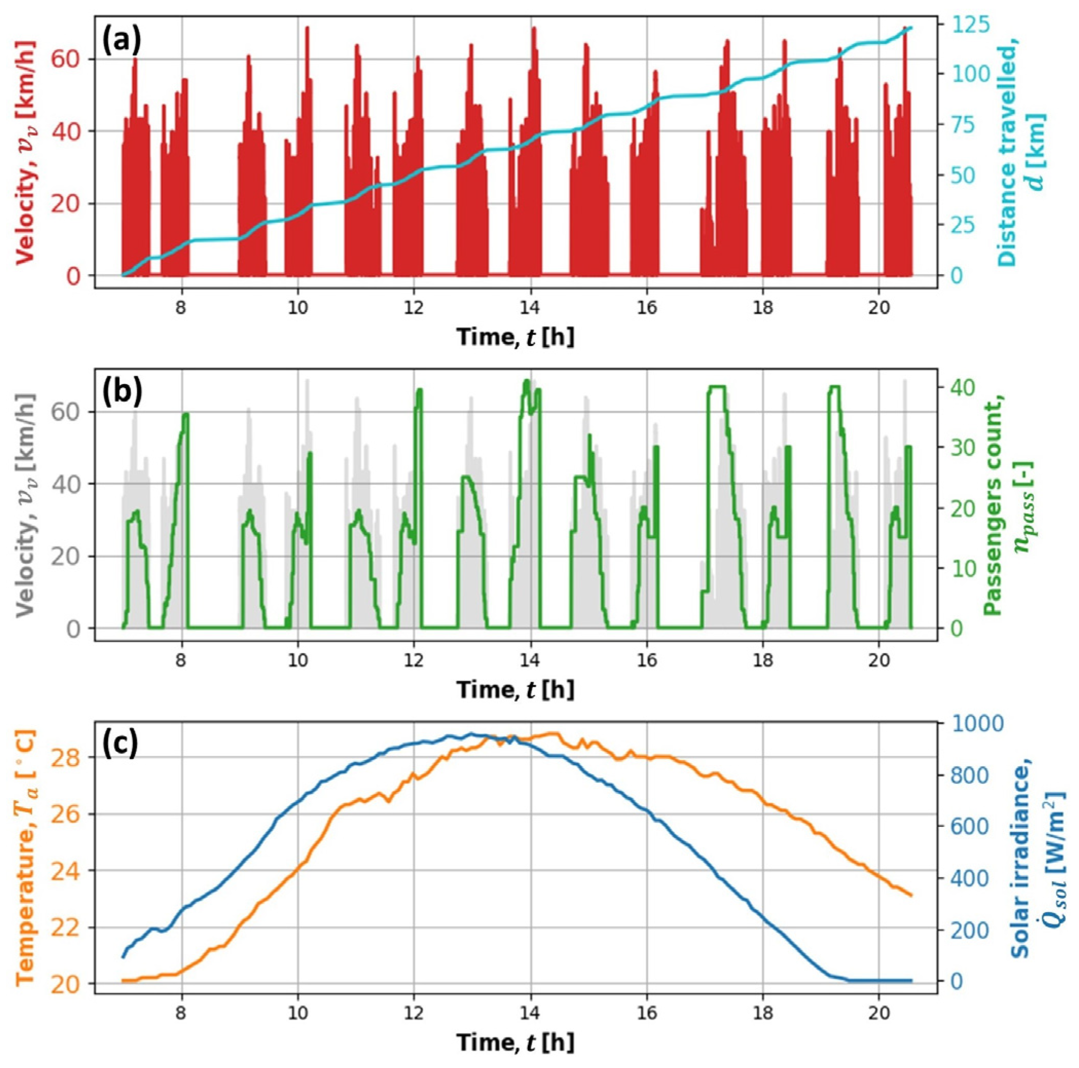
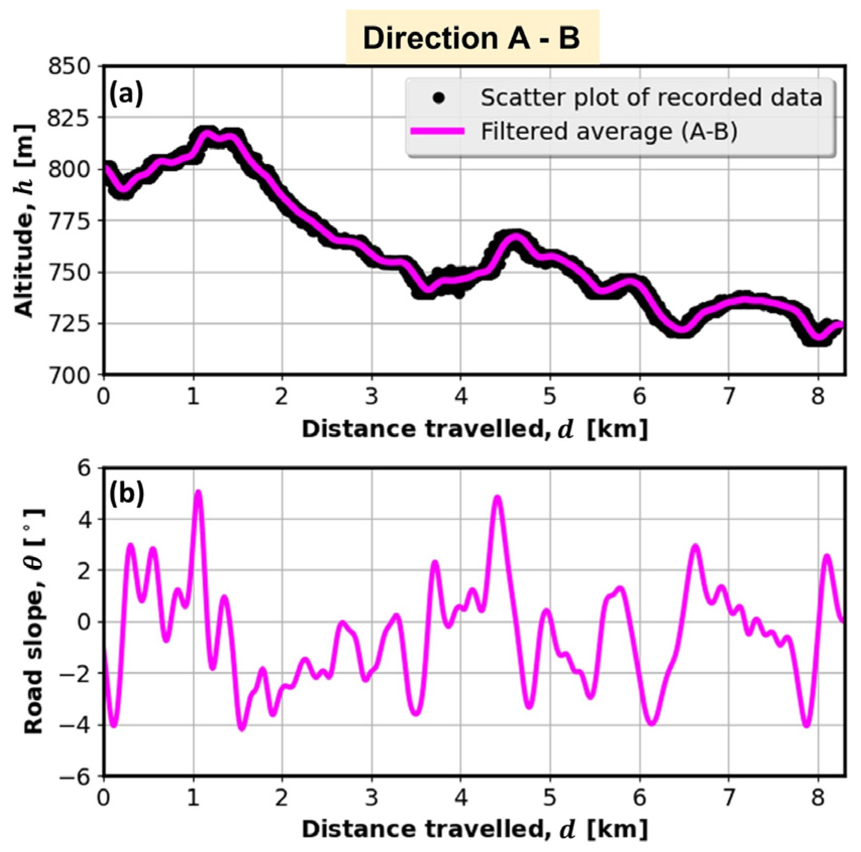
2.1. Recorded Driving Cycle and Energy Consumption Data

The driving cycle and energy consumption data were recorded on a single, 12 m e-bus operating on Route 15 in the city of Jerusalem [4]. The data were collected in the summer season in the period from 7 a.m. to 9 p.m., and they include timestamps, geographical coordinates (longitude, latitude, and altitude), velocity, distance traveled, cumulative battery energy consumption, and state of charge ($SoC$). The data sampling time was 1 s.

The considered dataset contains 14 trips in total (7 per each travel direction). The velocity profile along the day is shown in Figure 1a. The total distance traveled is approximately 122.5 km for a net operating time of 11.5 h. The corresponding reconstructed ridership profile is shown in Figure 1b. Finally, the actual ambient temperature ($T_a$) and solar irradiance (${\dot{Q}}_{sol}$) data profiles are shown in Figure 1c.

Figure 2a shows the plot of recorded and filtered altitude in relation to distance traveled for direction A–B and multiple trips. The reconstructed road slope profile is shown in Figure 2b. The driving direction A–B is characterized by mostly downhill driving with the road slope peaks up to 5°.

Figure 3 shows the recorded battery $SoC$ and cumulative energy consumption time profiles corresponding to the driving cycle from Figure 1a. These profiles are used as a reference for e-bus model parameterization. By linearly extrapolating the energy consumption profile over the whole $SoC$ range [0, 1], and subtracting the observed end values, one obtains a total battery capacity of 292.5 kWh, which equals 91% of the declared, new bus battery capacity of 324 kWh. The difference between the two battery capacity values can be attributed partly to nonlinear battery behavior, and partly to battery aging (the bus was produced in 2017).

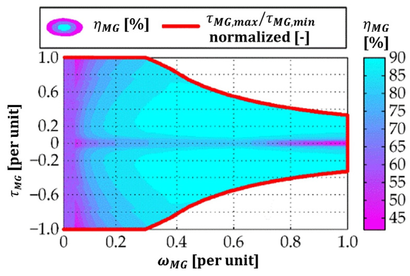
2.2. Physical Powertrain Model

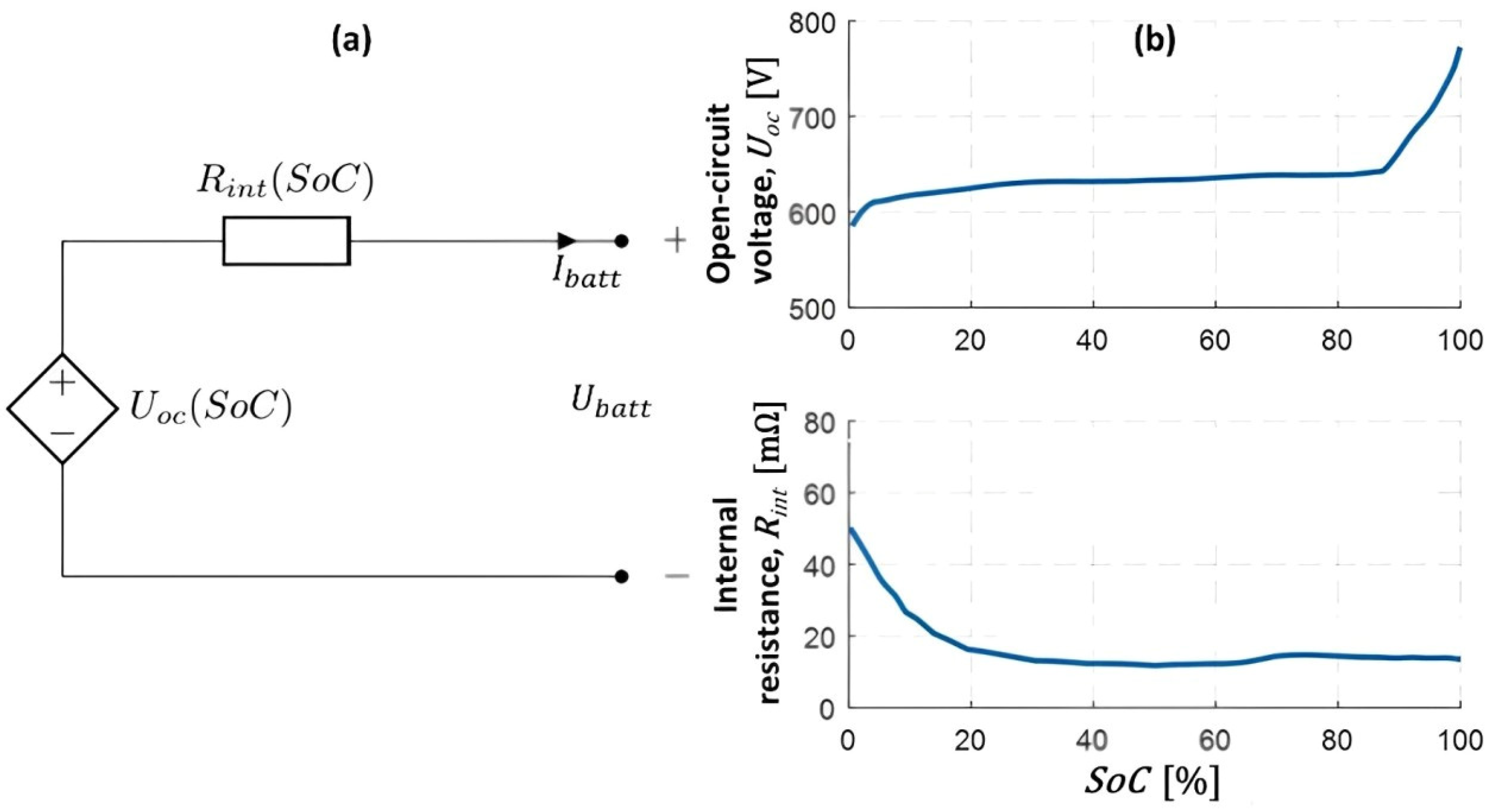
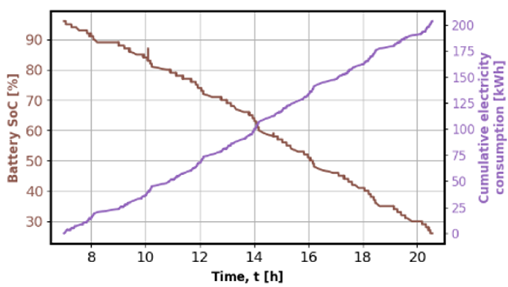
The powertrain of the considered fully electric city bus is modeled in a backward-looking manner, i.e., in the direction from the wheels towards the electric machine. The driving cycle-defined vehicle velocity (v_v), road slope (θ), and ridership inputs (n_pass), defined in Section 2.1, were fed into the vehicle longitudinal dynamics equations to calculate the total wheel torque and the wheel speed [24]:

$${\tau }_w=r_w{M}_v{\dot{v}}_v+r_w{R}_0{M}_{v}g\cos \left(\theta \right)+r_w{M}_{v}g\sin \left(\theta \right)+0.5r_w{\rho }_{air}{A}_f{C}_d{v}_v^2,$$

(1)

$${\omega }_w=\frac{v_v}{r_{w }},$$

(2)

where $r_w$ is the tire’s effective radius, $M_v=M_{v0}+M_{pass}$ is the sum of the empty vehicle mass (M_v0) and the total passengers’ mass ($M_{pass}$), $R_0$ is the rolling resistance coefficient, ${\rho }_{air}$ is the air density, $A_f$ is the bus frontal area, $C_d$ is the aerodynamical drag coefficient, and $g$ is the gravity acceleration. The individual passenger mass is estimated to be 68.125 kg to make a full bus with the passenger capacity of 80 match the declared maximum vehicle payload of 5450 kg. Therefore, the passenger mass $M_{pass}$ was calculated as $68.125·n_{pass}$.

The e-machine torque (${\tau }_{MG})$ and speed ${\omega }_{MG}$ are calculated as follows:

$${\tau }_{MG}=\frac{{\tau }_w{\eta }_{tr}^{k_t}\left({\tau }_w\right)+\frac{P_0\left({\omega }_w\right)}{{\omega }_w}}{i_0},$$

(3)

$${\omega }_{MG}=i_0{\omega }_w,$$

(4)

where $i_0$ is the final drive ratio, while ${\eta }_{tr}\left({\tau }_w\right)$ and $P_0\left({\omega }_w\right)$ are the drivetrain efficiency and the idle power loss maps [4], respectively, with k_t being defined as −1 for τ_w > 0 (motoring) and 1 for τ_w ≤ 0 (regenerative braking). The e-machine efficiency ${\eta }_{MG}$ is modeled by a map dependent on the e-machine speed and torque (see Figure 4, [4]), from which the e-machine power load to the battery is calculated as follows:

$$P_{MG}={\eta }_{MG}^k\left({\tau }_{MG},{\omega }_{MG}\right){\tau }_{MG}{\omega }_{MG},$$

(5)

where the exponent k depends on the e-machine operating mode: k = −1 for motoring ($P_{MG}>0$), and k = 1 for regenerative braking ($P_{MG}<0$).

2.3. Battery Model

The battery model is based on a single-cell model scaled up to the appropriate number of serially connected cells contained in the battery pack. The single-cell equivalent circuit model (ECM) has been developed based on the available data from the SAFT VL30PFe cell datasheet and insights from [25]. The ECM is shown in Figure 5a, and it consists of the source of the open-circuit voltage source ($U_{oc}$) and the internal resistance ($R_{int}$). Both parameters are made dependent on the cell $SoC$, as shown in Figure 5b. Temperature dependencies of both parameters are neglected since it is assumed that the e-bus includes an effective battery thermal management system.

The battery $SoC$ dynamics are described by the state equation:

$$\dot{SoC}=-\frac{I_{batt}}{Q_{\mathrm{m}\mathrm{a}\mathrm{x}}}=\frac{\sqrt{U_{oc}^2\left(SoC\right)-4R_{int}\left(SoC\right)P_{batt}}-U_{oc}\left(SoC\right)}{2Q_{\mathrm{m}\mathrm{a}\mathrm{x}}{R}_{int}\left(SoC\right)},$$

(6)

where I_batt is the battery current, Q_max is the battery charge capacity, and P_batt is the total battery power including the e-machine power P_MG given by Equation (5), and the powers of auxiliary devices (P_aux) (

Table 1. Values of nominal power (P_aux,N), duty cycle ($d_c$) and duty cycle period ${(t}_p$) of the modeled auxiliary devices.

Auxiliary Device	${\mathit{P}}_{\mathit{a}\mathit{u}\mathit{x},\mathit{N}}$ [W]	${\mathit{d}}_{\mathit{c}}$ [-]	${\mathit{t}}_{\mathit{p}}$ [s]
Servo steering	2500	0.09	400
Air compressor	2000	0.15	100
DC/DC converter with low voltage devices	184	1	N/A

) and HVAC system (P_HVAC) determined by the models described in the next two subsections:

$$P_{batt}=P_{MG}+{P_{aux}+P}_{HVAC}.$$

(7)

Note that the slowly changing $SoC$ variable is the only state variable of the overall e-bus backward-looking model (a quasi-static model). The battery charge capacity was obtained from the energy capacity E_max = 292.5 kWh as Q_max = E_max/U_oc ($SoC$ = 50%) = 459 Ah.

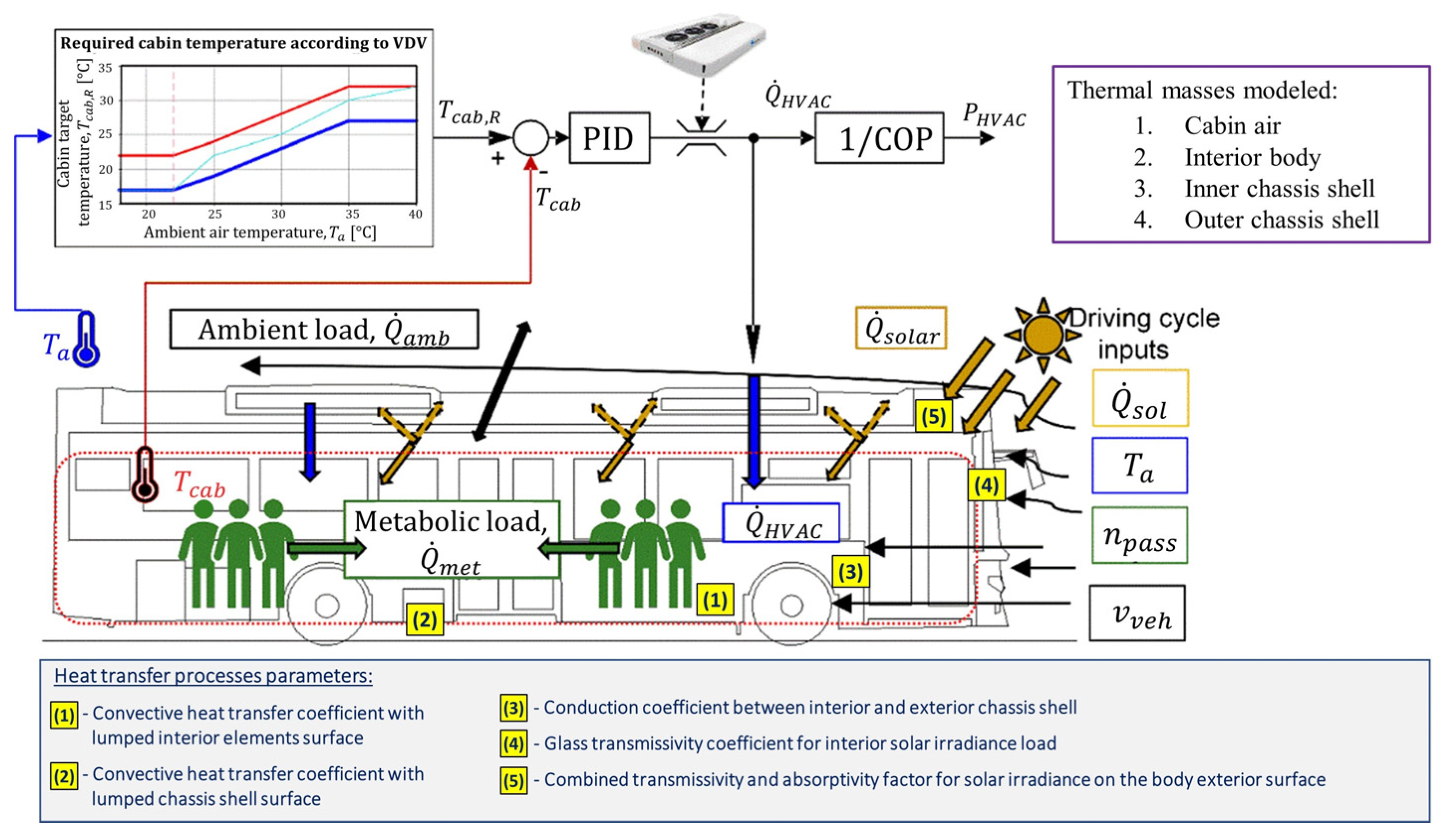
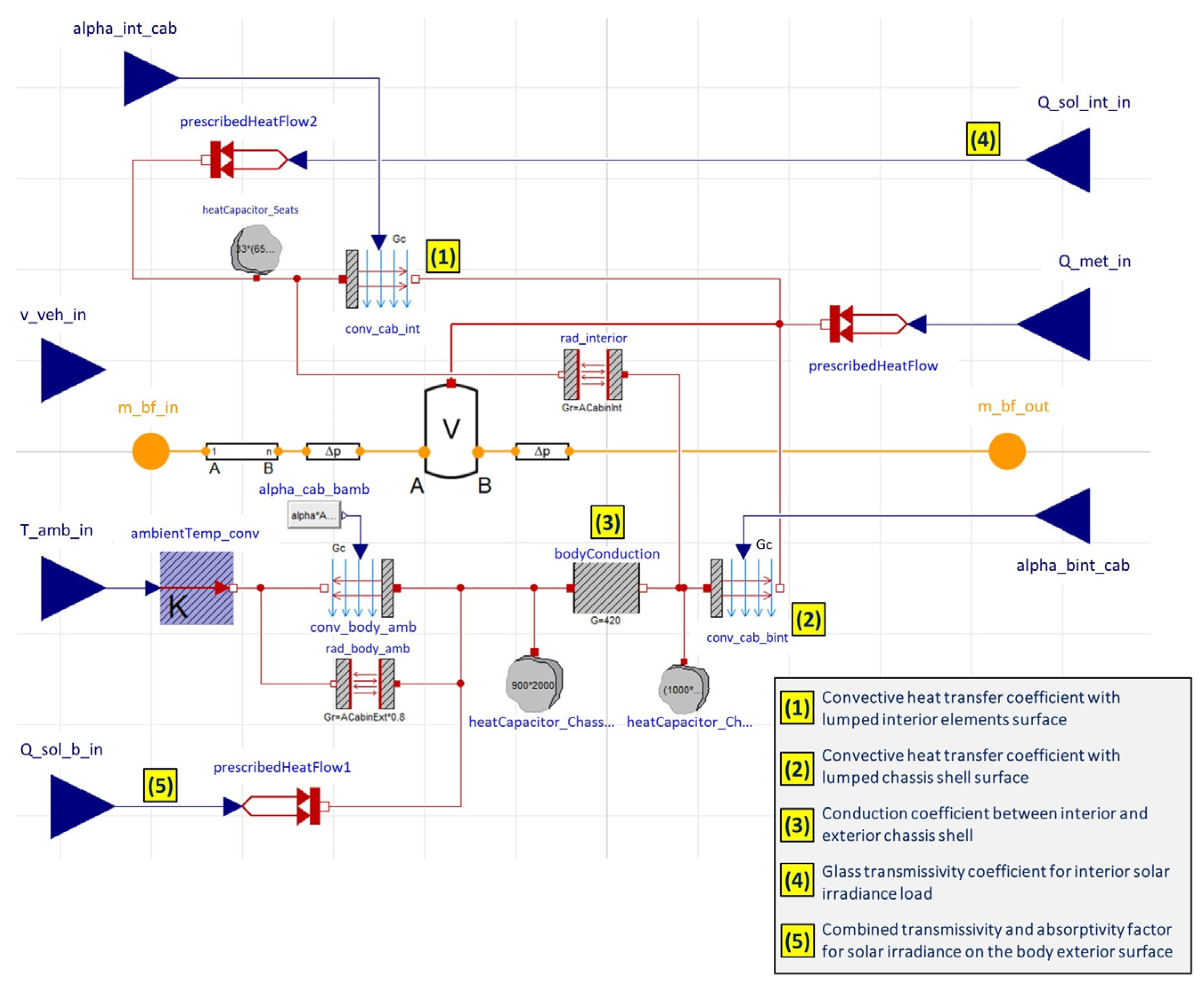
2.4. HVAC System Model

Apart from the e-bus powertrain itself, the HVAC system represents the most dominant battery energy consumer [26]. The ambient conditions such as ambient temperature and solar irradiance have a predominant effect on HVAC energy consumption, followed by climatic loads and user preferences [4,22]. It was reported in [27] that the impact of HVAC is such that it can reduce the range of an EV by up to 60% in cold weather and up to 33% in hot weather.

Since the considered driving cycle (Figure 1) corresponds to a summer day, the HVAC model parameterization is presented for the A/C mode. The overall thermal system is illustrated in Figure 6. A proportional–integral–derivative (PID) controller commands the cooling power ${\dot{Q}}_{HVAC}$ to maintain the cabin temperature T_cab at its reference value T_cab,R. The cooling power ${\dot{Q}}_{HVAC}$ is limited in accordance with the HVAC datasheet [4]. The reference variable T_cab,R is generated with dependence on the ambient temperature T_a (see the cyan line in Figure 6), which is set to fall between the bounds defined by VDV 236:2015 guidelines for public transport (red and blue lines). Based on the assumptions of fast HVAC system response constant coefficient of performance (COP = 1.8), the HVAC power consumption P_HVAC from Equation (7) was determined as ${\dot{Q}}_{HVAC}/COP$.

The thermal dynamics model includes four thermal masses (Figure 6 [4]). The model is implemented in Dymola 2018 FD01 as illustrated in Figure 7. The model inputs include ambient temperature $\left(T_a\right)$, solar irradiance (${\dot{Q}}_{sol}$), vehicle velocity (v_v), and ridership (n_pass).

Certain parameters of the cabin thermal model were difficult to determine or estimate due to either lack of available data or complex parameter dependencies [4]. The unknown cabin thermal model parameters were determined through optimization by using modeFRONTIER 2018R2 software. The optimization setup is illustrated by the block diagram shown in Figure 8. The overall model used in the optimization setup in Figure 8 includes not only the Dymola thermal model but also the powertrain model implemented in Python. This is to obtain simulation responses of the battery $SoC$ and the overall energy consumption E_sim = ∫P_batt dt, which were compared with the recorded $SoC$ and energy consumption responses to generate the corresponding RMS errors fed to the optimization genetic algorithm MOGA-II to minimize those errors. The two-objective optimization resulted in a Pareto frontier of optimal solutions. The selected solution corresponds to a low energy consumption RMS error, and it resulted in a favorable overall fit accuracy (partly because of a better resolution of the recorded energy consumption signal than the recorded $SoC$ signal).

The simulation profiles of e-bus model variables, obtained through the cabin thermal model parameter optimization and shown in Figure 9, were further used to optimize the parameters of an HVAC regression model. The regression model is quadratic but linear in parameters and its inputs correspond to the inputs of the cabin thermal model ($T_a$, ${\dot{Q}}_{sol}$, v_v and n_pass). The Matlab function stepwiselm available within the Statistics and Machine Learning Toolbox was used to select the model features and optimize its parameters. The selected model is given by the following:

$$P_{HVAC}={\beta }_0+{\beta }_1{T}_a+{\beta }_2{\dot{Q}}_{sol}+{\beta }_3{n}_{pass}+{\beta }_4{v}_{veh}+{\beta }_{14}{T}_a{v}_{veh}+{\beta }_{22}{{\dot{Q}}_{sol}}^2.$$

(8)

The comparative responses of actual and simulation responses of $SoC$, energy consumption, and HVAC power, shown in Figure 9, indicate very good modeling accuracy on the dataset used in model parameterization (training).

The above HVAC modeling approach was demonstrated for the particular case of 12 m e-bus and A/C operating mode. The approach may be extended to other e-bus configurations and operating conditions without reoptimizing the physical model parameters. This is illustrated in Appendix A for examples of heat pump mode (i.e., winter conditions) and an 18 m e-bus.

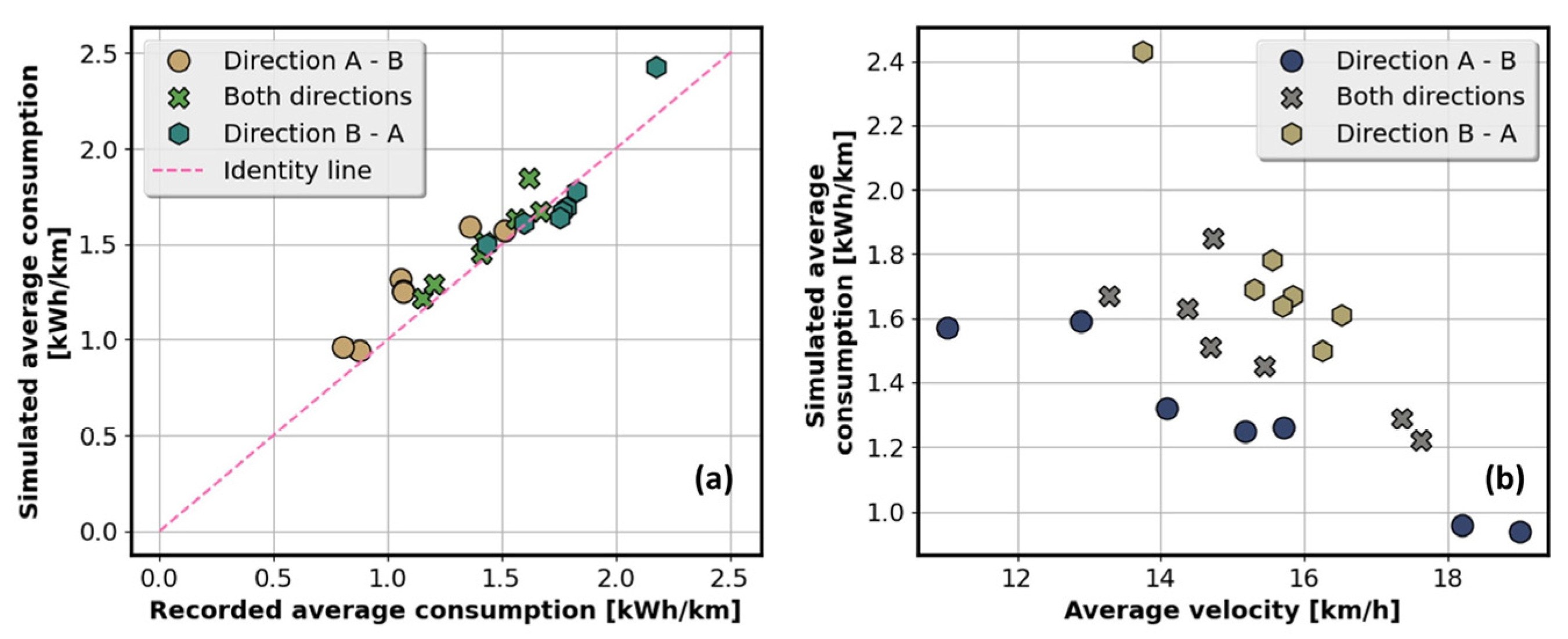
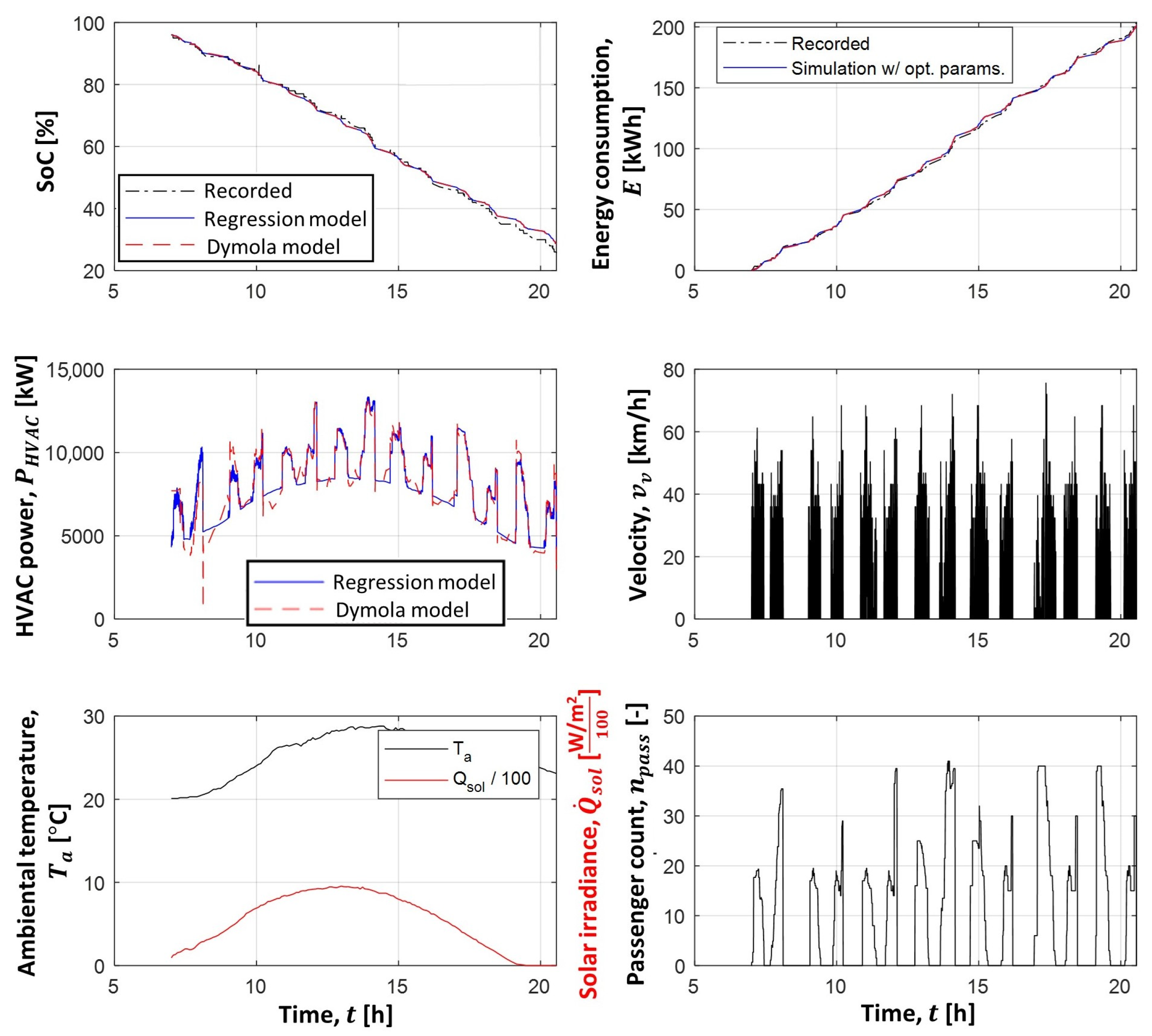
2.5. E-Bus Model Validation

For an unbiased assessment of modeling accuracy, the overall e-bus model was also validated against a couple of other datasets (corresponding to different days of operation of the same bus on the same route during the same summer month). The results of the first validation, shown in Figure 10a, confirm the very good modeling accuracy, characterized by the mean absolute error of $SoC$ prediction (${MAE}_{SoC}$) being equal to 0.90%.

However, the model performance degraded for the second validation (Figure 10b) in terms of the occurrence of $SoC$ and energy consumption offsets during a relatively long bus pause (dwell time) at the end station after the second driving mission (i.e., after 8 a.m.; see also the velocity profile in Figure 9). This is reflected in the increase in the corresponding MAE_SoC indicator from 0.9% to 4.09%. It is hypothesized that, unlike in the previous two datasets, the HVAC was shut down during the morning hours since the ambient temperature was around the room temperature. Because the model presumes that the HVAC was active during the whole operation period, its $SoC$ and energy consumption persistently change, thus accumulating the offset during the morning pause. In order to check the above hypothesis, the HVAC is shut down in the model in the period from 7 a.m. to 10 a.m. The corresponding results shown in Figure 10c indicate that the modeling accuracy is significantly improved when compared to the original response in Figure 10b, which is reflected in the reduction of ${MAE}_{SoC}$ indicator from 4.09% to 1.81%. A small offset was, though, still present in the $SoC$ and energy consumption results around 10 a.m., which is expected to be predominantly caused by the fact that the exact HVAC shut-down period is not known from the available data.

Once the e-bus model is successfully validated, it can be used as a basis for energy consumption sensitivity analysis for a wide range of scenarios and operating conditions (including those not covered by the particular recorded data sets). Such an analysis is presented in [4]. It is reduced here to the main and compact plots shown in Figure 11. The specific energy consumption (Figure 11a) varies significantly partly due to the effect of road slope (the consumption is lower for mostly downhill driving in Direction A–B), and partly due to the varying ambient, ridership, and traffic conditions (the consumption scatters for individual route directions). The traffic condition influence is substantiated by the correlation between the specific energy consumption and the average vehicle velocity (Figure 11b). The individual direction-specific consumptions vary in the range from around 0.9 to 2.4 kWh/km, while for the two-way trips they fall in the range from 1.2 to 1.8 kWh/km. The good modeling accuracy is confirmed through good alignment of simulation vs. recorded values with the ideal 1:1 line in Figure 11a. Quantitatively, the plot in Figure 11a is represented by Pearson’s correlation coefficient of 0.95 and the coefficient of determination is R² = 0.85, which are quite close to the ideal value of 1.

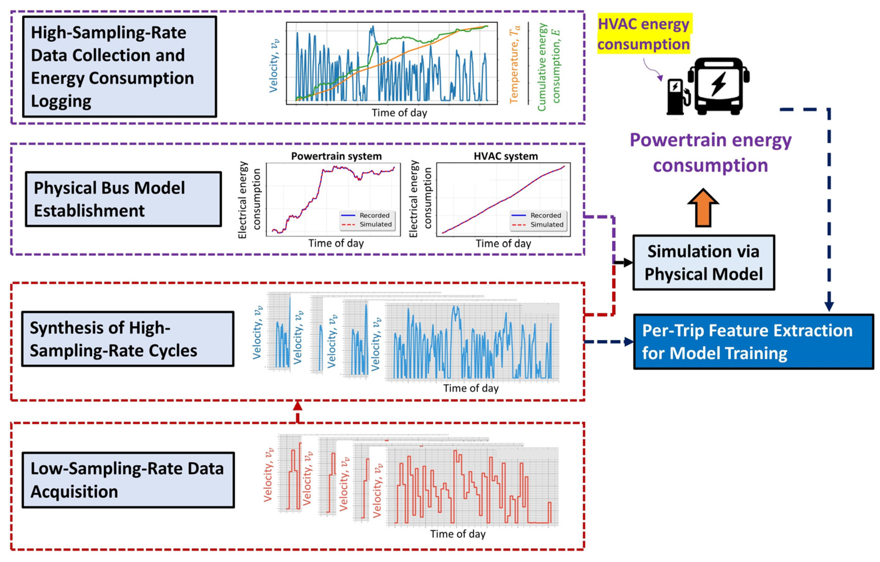
3. Data Collection for Data-Driven E-Bus Modeling

3.1. Data Collection Framework

In the absence of a wide set of recorded e-bus energy consumption data, the framework depicted in Figure 12 was employed to generate the data needed for data-driven modeling. Initially, the single-route high-sampling-rate (1 Hz) data were acquired for parametrization and validation of the physical e-bus model (Section 2).

At the same time, low-sampling-rate data (at around 0.25 Hz) were collected from a fleet of around 300 conventional buses operating on 29 routes in the same city over the period of one month. The recorded low sampling rate data were then transformed into the corresponding set of representative high sampling rate driving cycles corresponding to trips between two end stations. Those driving cycles were then fed to the developed physical e-bus model to obtain the energy consumption data. The transformation was based on the Markov chain synthesis method proposed in [13].

Finally, a wide set of trip-based statistical features (e.g., mean velocity, number of bus station stops, average ridership, trip duration, initial $SoC$, etc.) were extracted from the synthetic driving cycles. They were paired with the simulation data on energy consumption to form a dataset employed for the development of a data-driven model in Section 4 and Section 5.

3.2. Data Collection Framework

In total, 4057 synthetic driving cycles were generated [13]. Each cycle is unique with respect to route (considering diverse road and traffic conditions, including varying road grades) and trip (considering fluctuating traffic and ridership conditions). Additionally, each driving cycle has a distinct initial battery $SoC$.

To rigorously assess the data-driven model extrapolation ability (i.e., its generalization properties), four additional sets of driving cycles were derived from the basic set of synthetic driving cycles (Set #1):

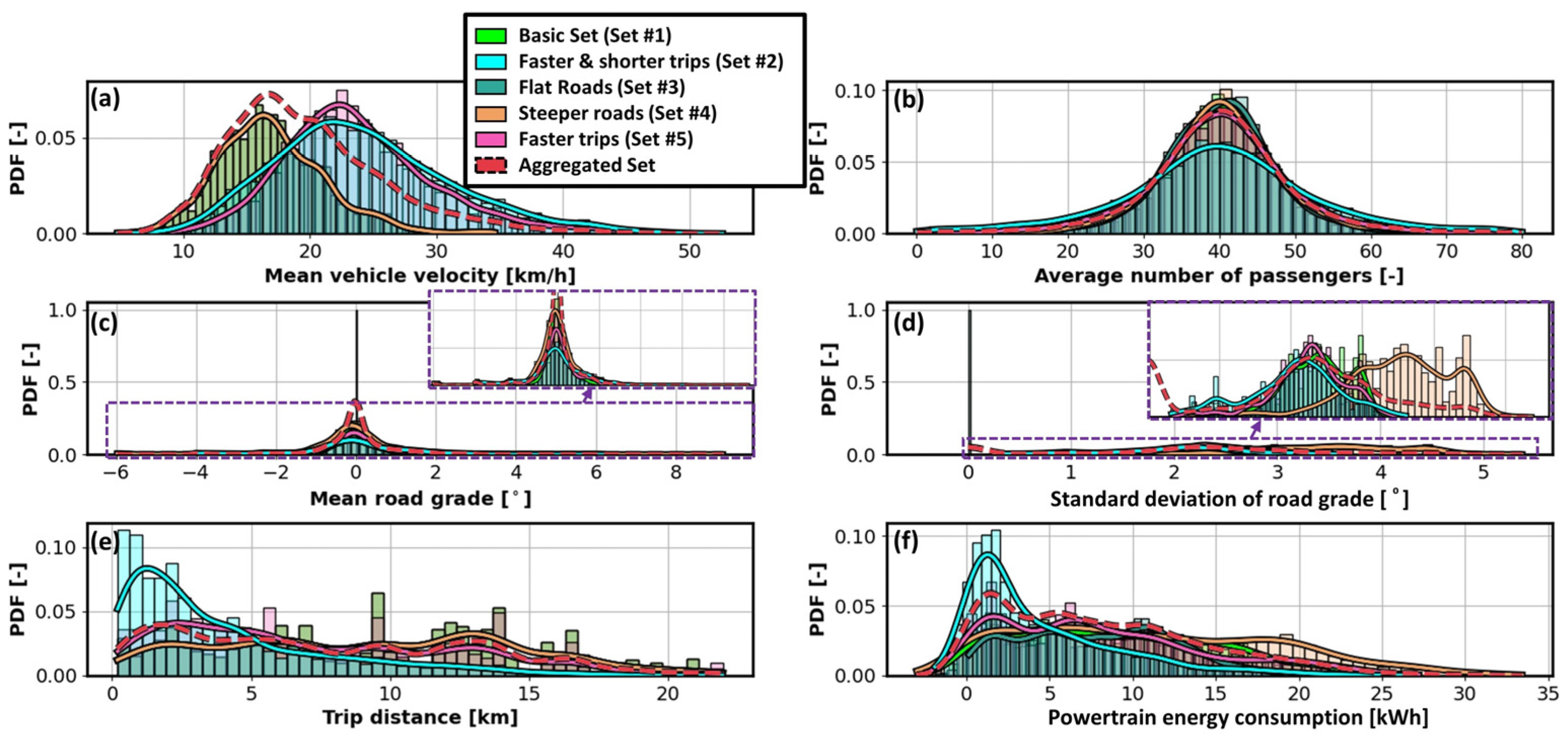
• Set #2: Faster and shorter trips: For each trip, the mean velocity of every bus station-to-station segment is amplified by 50% and the traveled distances are randomly reduced;
• Set #3: Flat roads: the road slope is set to zero;
• Set #4: Steeper roads scenario: the road grade profile is scaled up by 50%;
• Set #5: Faster trips: The mean velocity of each station-to-station segment is amplified by 50%.

Figure 13 shows histograms of the main driving cycle features for all the five individual datasets and the corresponding aggregate dataset. The corresponding histogram of powertrain energy consumption per trip is given, as well. When compared to the basic dataset (Set #1), the modified datasets extend the range of features, thus making the aggregate dataset wider and flatter.

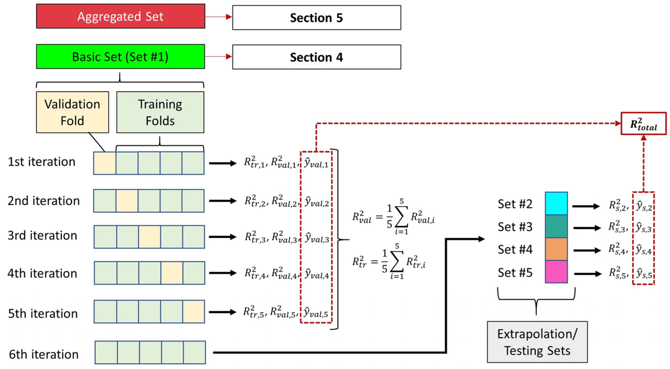
4. Feature Selection

Feature selection is an integral component of machine learning and data analytics. It is aimed at enhancing the model’s accuracy and simplicity by identifying and retaining only the most relevant features. The presented feature selection method corresponds to e-bus powertrain (and auxiliary devices) modeling only because HVAC modeling represents an independent and straightforward trip-based modification of the approach presented in Section 2 (see Section 5).

4.1. Data Collection Framework

Two metrics were employed to evaluate energy consumption modeling accuracy [28]: (i) root mean square error ($RMSE$) and (ii) coefficient of determination ($R^2)$. To reduce the number of model inputs, the powertrain energy consumption is normalized with respect to the traveled distance. The output predicted by such a normalized model (i.e., specific energy consumption in kWh/km) is in the final modeling stage multiplied by the traveled distance to calculate the absolute energy consumption in kWh. The model performance metrics $R^2$ and $RMSE$ metrics are computed with respect to the final model output, i.e., the absolute energy consumption.

For the purpose of model evaluation, a five-fold cross-validation method was applied to the basic dataset (Set #1, Section 3), as depicted in Figure 14. The basic dataset was randomly partitioned into five sections, which are termed folds. In each iteration of the cross-validation method, a single fold was designated for model validation, with the remaining four serving for training. After five iterations corresponding to different folds (Figure 14), this process yielded individual scores $R_{tr,i}^2$ and $R_{val,i}^2$, i = 1, …, 5, related to training and validation in each iteration, from which lumped/average scores $R_{tr}^2$ and $R_{val}^2$ were derived (Figure 14).

In the sixth iteration, the model is trained on the whole (unpartitioned) basic dataset. The obtained model is then applied to the extrapolation datasets (Sets #2–#5 from Section 3), thus resulting in the validation scores $R_{s,j}^2$, j = 2, …, 5 (Figure 14). Finally, the combined validation score $R_{total}^2$ is obtained from the residuals calculated by merging the predicted outputs from the validation iterations (${\widehat{y}}_{val,i}$ for $i=1,\dots 5$) with the predicted values for the extrapolation sets (${\widehat{y}}_{s,j}$ for $j=2,\dots 5$), and subtracting them from their true-value counterparts. The described validation process (Figure 14) was applied to determine the $RMSE$ metrics, as well. In addition to the basic data set (see below), it was also applied to the aggregate dataset (Section 5 and Section 6).

4.2. Quadratic Regression Model

Feature selection was conducted by using the following linear-in-parameter quadratic model:

$$\begin{gathered} \widehat{y}={\beta }_0+{\beta }_1{X}_1+{\beta }_2{X}_2+{\beta }_3{X}_3+{\beta }_4{X}_4+{\beta }_5{X}_1^2+{\beta }_6{X}_2^2+{\beta }_7{X}_3^2+{\beta }_8{X}_4^2+{\beta }_9{X}_1{X}_2+ \\ {\beta }_{10}{X}_1{X}_3+{\beta }_{11}{X}_1{X}_4+{\beta }_{12}{X}_2{X}_3+{\beta }_{13}{X}_2{X}_4+{\beta }_{14}{X}_3{X}_4, \end{gathered}$$

(9)

where $\widehat{y}$ is the dependent variable (here, specific powertrain consumption), $X_1,X_2,\dots ,X_n$ are the predictor variables (with n = 4 in the example of Equation (9)), ${\beta }_0$ is the $y$-intercept parameter, and ${\beta }_1,{\beta }_2,\dots ,{\beta }_m$, $m=2n+\frac{n(n-1)}{2}$, are the model parameters corresponding to individual features and identified by the least square method [29].

The considered predictor variables include (see dark blue block in Figure 12): the total number of route stations $N_{stations}$, the number of stations that the bus actually stopped at, $N_{stops}$, the ratio of stopping to total stations ${\rho }_{stops}=N_{stops}/N_{stations}$, mean velocity ${\mu }_v$, average ridership ${\overline{n}}_{pass}$ and standard deviation of ridership ${\sigma }_{pass}$, trip duration $t_{trip}$, trip distance $d_{trip}$, the initial state of charge ${SoC}_{init}$, mean road grade ${\mu }_{rg}$, and the standard deviation of road grades ${\sigma }_{rg}$. With this set of n = 11 predictor variables, the number of quadratic model features equals m = 77.

4.3. Feature Selection Techniques

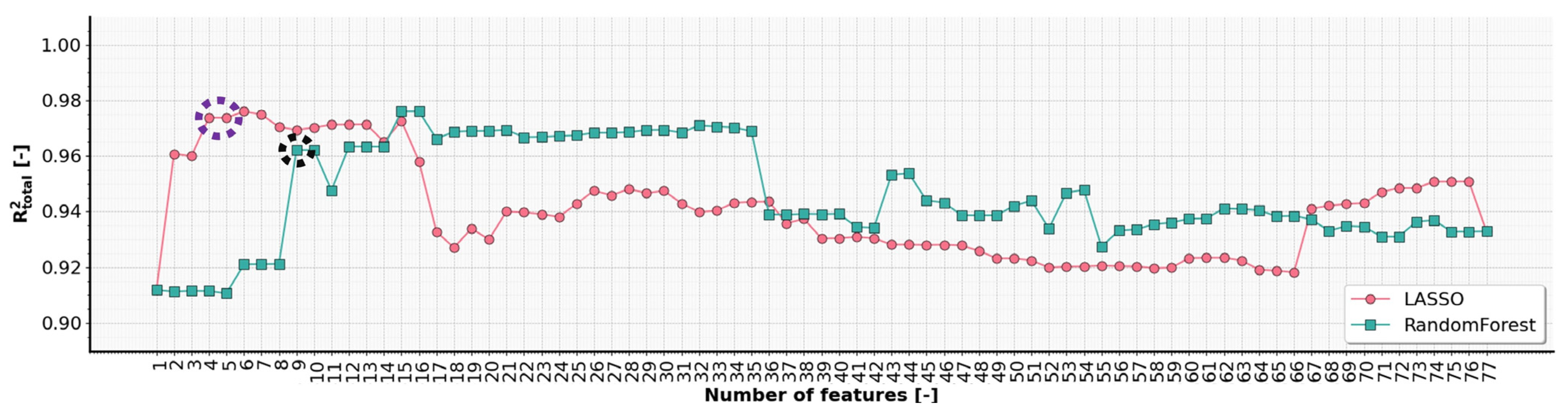
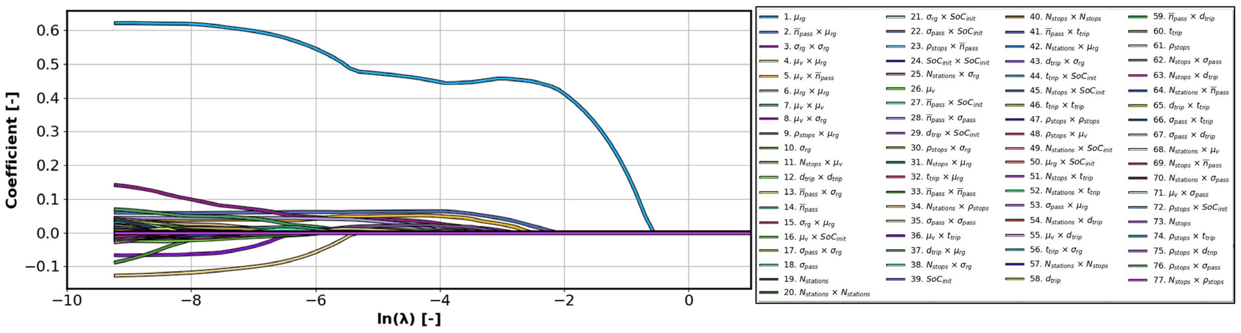
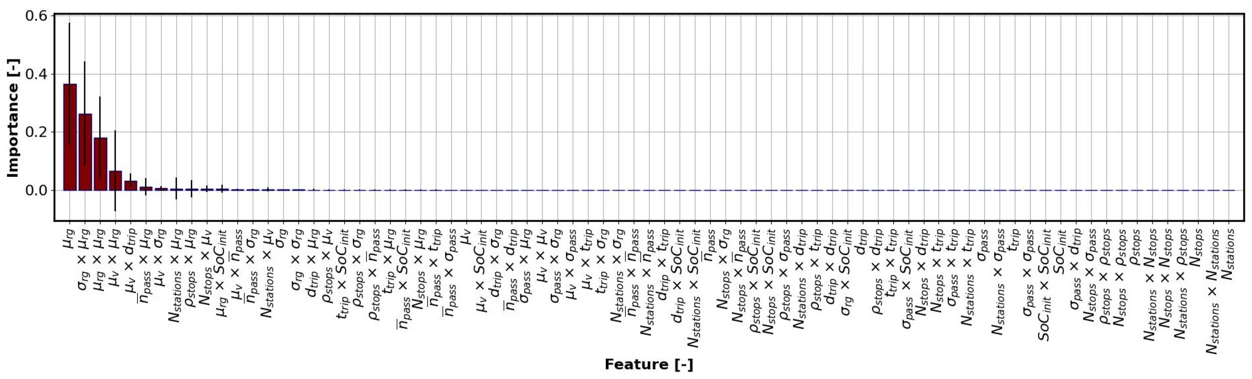
4.3.1. LASSO and RANDOM Forest Importance Methods

The LASSO (Least Absolute Shrinkage and Selection Operator) technique applies a penalty to the absolute values of regression parameters ${\beta }_i$, $i=1,\dots ,m$, as an extension of the least square cost function, thus encouraging parameters corresponding to non-influential features to diminish ([30]; Figure 15). This shrinkage mechanism is controlled by the penalty coefficient lambda λ. As λ grows, more model parameters converge to zero.

Random forest importance approach assigns importance scores to features based on their frequency in splitting data, indicating their contribution to the prediction accuracy. This relative feature importance is illustrated in Figure 16.

The quadratic regression model was re-trained by sequentially adding individual features based on their significance ranking provided by LASSO and Random forest importance approaches. The results are shown in Figure 17 based on the $R_{total}^2$ validation metrics introduced in Section 4.1. They indicate that the LASSO approach achieves peak performance with a smaller number of features compared to the Random forest importance method.

4.3.2. Wrapper Methods

Wrapper methods select the best feature subsets by building and evaluating models [30]. Forward feature selection, Backward feature elimination, and Stepwise regression are characteristic methods from this category. Each method identifies an optimal set of regression model features based on the Bayesian Information Criterion ($BIC$):

$$BIC=k \mathrm{l}\mathrm{n}\left({\sigma }^2\right)+\left(m+1\right)\mathrm{l}\mathrm{n}\left(k\right),$$

(10)

where $m+1$ represents the number of model parameters (including the intercept), $k$ signifies the number of observations (sample size), and ${\sigma }^2$ represents the average of the squared differences between the observed values and the values predicted by the model, quantifying the model prediction error. A lower $BIC$ index suggests a better model fit.

Forward Feature Selection begins with no features and continues with successively adding them based on model fit improvement until the $BIC$ value increase surpasses a threshold of 100. Backward Feature Elimination begins with all features and removes them successively to improve the model while stopping when the $BIC$ falls below the threshold of 150. Stepwise regression combines both methods, adjusting features based on fit with the adding threshold of 450 and the removal threshold of 400. The above thresholds have been determined heuristically to provide a good trade-off of model performance and complexity (i.e., number of terms).

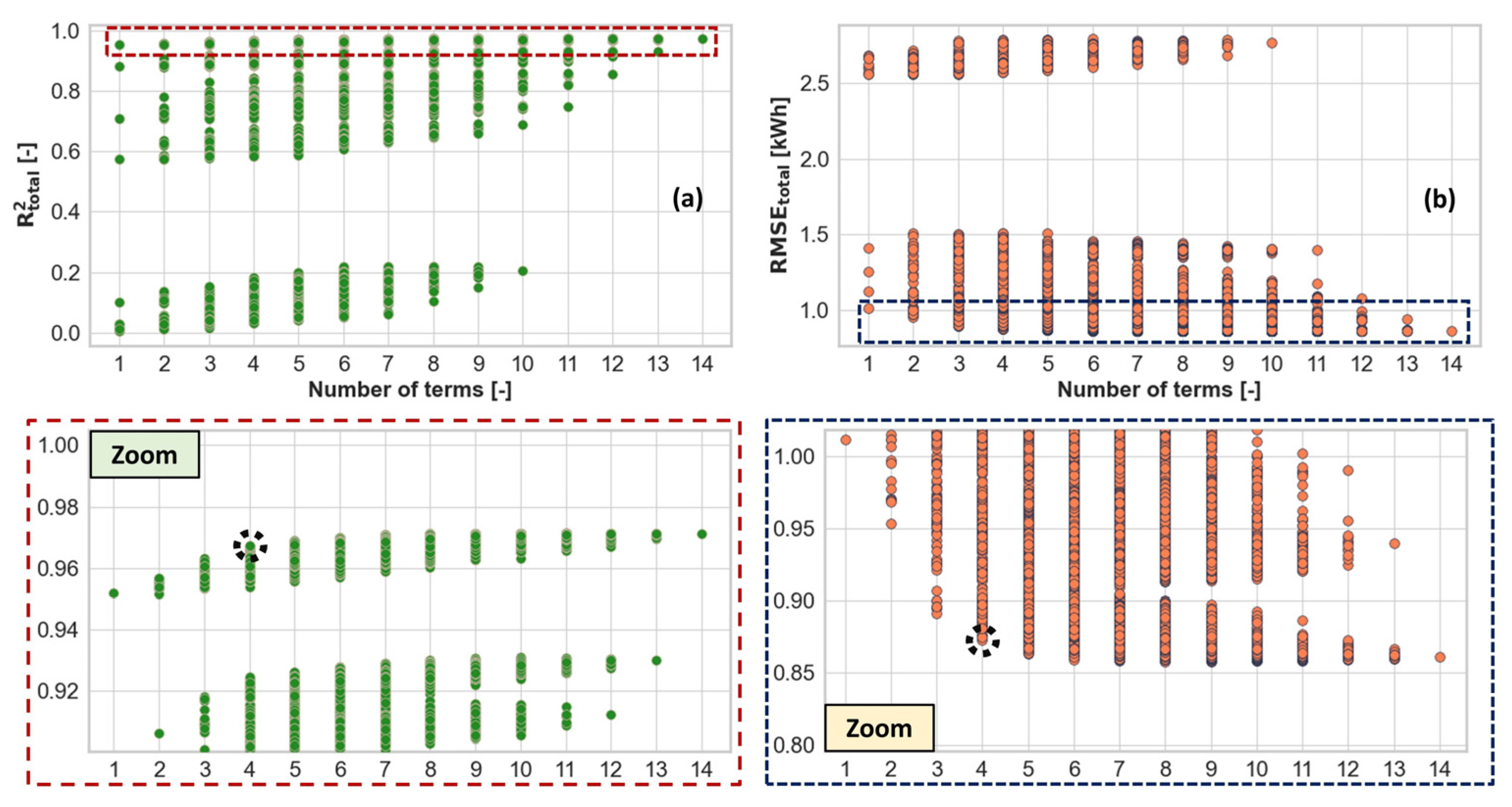
4.3.3. Best Subset Method

The best subset method searches through all combinations of features to identify the optimal model subset. Due to the high computational demand, the number of predictor variables is reduced to the following $n=4$ variables highlighted by feature selection results in Figure 15 and Figure 16: mean road grade, standard deviation of road grade, average number of passengers, and mean velocity. This leads to the quadratic regression model given by Equation (9) and having $m=14$ features. Consequently, 16,383 distinct linear regression models can be produced. The performance of each model, depicted in Figure 18 by a point, is represented by the values of validation metrics $R_{total}^2$ and ${RMSE}_{total}$.

4.4. Comparative Analysis of Model Gained by Various Feature Selection Methods

Different feature selection methods yield multiple candidate feature sets, which are summarized in

Table 2. Comparative performance metrics of optimal models obtained by various feature selection methods.

Number of Features	Selected Features	${\mathit{R}}_{\mathit{t}\mathit{r}}^2$ ${\mathit{R}\mathit{M}\mathit{S}\mathit{E}}_{\mathit{t}\mathit{r}}$	${\mathit{R}}_{\mathit{v}\mathit{a}\mathit{l}}^2$ ${\mathit{R}\mathit{M}\mathit{S}\mathit{E}}_{\mathit{v}\mathit{a}\mathit{l}}$	${\mathit{R}}_{\mathit{s},2}^2$ ${\mathit{R}\mathit{M}\mathit{S}\mathit{E}}_{\mathit{s},2}$	${\mathit{R}}_{\mathit{s},3}^2$ ${\mathit{R}\mathit{M}\mathit{S}\mathit{E}}_{\mathit{s},3}$	${\mathit{R}}_{\mathit{s},4}^2$ ${\mathit{R}\mathit{M}\mathit{S}\mathit{E}}_{\mathit{s},4}$	${\mathit{R}}_{\mathit{s},5}^2$ ${\mathit{R}\mathit{M}\mathit{S}\mathit{E}}_{\mathit{s},5}$	${\mathit{R}}_{\mathit{t}\mathit{o}\mathit{t}\mathit{a}\mathit{l}}^2$ ${\mathit{R}\mathit{M}\mathit{S}\mathit{E}}_{\mathit{t}\mathit{o}\mathit{t}\mathit{a}\mathit{l}}$
LASSO
4	${\mu }_{rg}$, ${\sigma }_{rg}^2$, ${\mu }_v\times {\mu }_{rg}$, ${\mu }_v\times {\overline{n}}_{pass}$	0.9777 0.8873	0.9776 0.8862	0.9650 0.8720	0.9829 0.5911	0.9575 1.5901	0.9592 1.2487	0.9738 1.0126
5	${\mu }_{rg}$, ${\sigma }_{rg}^2$, ${\mu }_v\times {\mu }_{rg}$, ${\mu }_v\times {\overline{n}}_{pass}$,${\overline{n}}_{pass}\times {\mu }_{rg}$	0.9776 0.8883	0.9776 0.8881	0.9656 0.8649	0.9816 0.6124	0.9568 1.6032	0.9601 1.2350	0.9737 1.0153
Random forest importance
9	${\mu }_{rg}$, ${\mu }_{rg}^2$, ${\sigma }_{rg}\times {\mu }_{rg}$, $N_{stations}\times {\mu }_{rg}$, ${\mu }_v\times {\mu }_{rg}$, ${\mu }_v\times d_{trip}$, $N_{stops}\times {\mu }_v$, ${\overline{n}}_{pass}\times {\mu }_{rg}$, ${\mu }_v\times {\sigma }_{rg}$	0.9752 0.9346	0.9750 0.9381	0.9645 0.8783	0.9312 1.185	0.9374 1.9290	0.9576 1.2731	0.9621 1.1896
Forward selection
8	${\mu }_{rg}$, ${\mu }_v\times {\overline{n}}_{pass}$, ${\sigma }_{rg}^2$, ${\mu }_{rg}^2$, ${\mu }_v\times {\mu }_{rg}$, ${\overline{n}}_{pass}\times {\mu }_{rg}$, ${\sigma }_{rg}$, $t_{trip}\times {\mu }_{rg}$	0.9787 0.8673	0.9785 0.8682	0.9636 0.8895	0.8790 1.5719	0.9625 1.4927	0.9556 1.3017	0.9638 1.1652
Backward elimination
10	${\mu }_{rg}$, ${\mu }_v^2$, ${\mu }_v\times {\overline{n}}_{pass}$, ${\mu }_v\times {\sigma }_{rg}$,${\mu }_v\times {\mu }_{rg}$,${\overline{n}}_{pass}\times {\mu }_{rg}$, ${\overline{n}}_{pass}\times {SoC}_{init}$, ${\sigma }_{pass}\times {\sigma }_{rg}$, ${\sigma }_{rg}^2$, ${\mu }_{rg}^2$	0.9781 0.8787	0.9780 0.8788	0.9656 0.8640	0.9464 1.0462	0.9617 1.5088	0.9571 1.2799	0.9710 1.0761
Stepwise regression
6	${\mu }_{rg}$, ${\mu }_v\times {\overline{n}}_{pass}$, ${\sigma }_{rg}^2$, ${\mu }_{rg}^2$, ${\mu }_v\times {\mu }_{rg}$, ${\overline{n}}_{pass}\times {\mu }_{rg}$	0.9783 0.8755	0.9782 0.8752	0.9647 0.8757	0.9840 0.5719	0.9660 1.4222	0.9569 1.2825	0.9760 0.9839
Best subset
3	${\mu }_{rg}$, ${\sigma }_{rg}^2$, ${\mu }_v\times {\overline{n}}_{pass}$	0.9778 0.8860	0.9777 0.8849	0.9662 0.8567	0.9828 0.5923	0.9574 1.5919	0.9591 1.2504	0.9739 1.0104
4	${\mathit{\mu }}_{\mathit{r}\mathit{g}}$, ${\mathit{\mu }}_{\mathit{r}\mathit{g}}^2$, ${\mathit{\sigma }}_{\mathit{r}\mathit{g}}^2$, ${\mathit{\mu }}_{\mathit{v}}\times {\overline{\mathit{n}}}_{\mathit{p}\mathit{a}\mathit{s}\mathit{s}}$	0.9784 0.8727	0.9784 0.8721	0.9639 0.8855	0.9825 0.5978	0.9666 1.4091	0.9546 1.3161	0.9755 0.9922
5	${\mu }_{rg}$, ${\mu }_{rg}^2$, ${\mu }_{rg}\times {\sigma }_{rg}$, ${\sigma }_{rg}^2$, ${\mu }_v\times {\overline{n}}_{pass}$	0.9786 0.8694	0.9785 0.8690	0.9642 0.8817	0.9821 0.6047	0.9681 1.3774	0.9547 1.3153	0.9759 0.9862
6	${\mu }_{rg}$, ${\overline{n}}_{pass}$, ${\mu }_{rg}^2$, ${\mu }_{rg}\times {\mu }_v$, ${\sigma }_{rg}^2$, ${\mu }_v^2$	0.9781 0.8782	0.9781 0.8782	0.9666 0.8521	0.9823 0.6010	0.9662 1.4178	0.9582 1.2630	0.9763 0.9817

Note: All $RMSE$ values are given in kWh.

. Four candidate sets, including from 3 to 6 features, are identified by the best subset method as a good trade-off of modeling accuracy and simplicity (see Figure 18a). Although the LASSO and Random forest metrics peaks occur for the sets of 6 and 15 features, respectively, simpler sets that are still close to the performance peak sets are preferred in Table 2 (see configurations marked in purple and black in Figure 17), which is influenced by the best subset approach emphasis on fewer features. The wrapper methods are each represented by a single optimal configuration.

Out of the total of 10 configurations listed in Table 2, the four-feature one given by the best subset method (given in bold in Table 2 and marked in Figure 18) was selected for further analysis in Section 5. This is because its score $R_{total}^2$ = 0.9755 nearly matches the top score $R_{total}^2$ = 0.9763 of the best-subset model with six features. Moreover, minimal variance in $R^2$ (and $RMSE$) among different data sets (see metrics R_s,2,…, R_s,4 in Table 2) points to a consistent performance of the selected best subset model, along with its good interpretability (e.g., there is only a single interaction term—the one between mean velocity and average ridership).

5. Final Model and Its Performance Assessment

In Section 4, powertrain model features were selected (see the bolded row of Table 2), and the model was trained and validated on the basic dataset and then tested on four separate (extrapolation) datasets. Herein, a combined/aggregate dataset, including all the five data subsets (see Figure 13), was used for both training and validation, i.e., the training/validation folds in Figure 14 were extracted from the aggregated dataset. This approach aims to improve the modeling accuracy and allows for a direct performance comparison between the linear regression model and more complex machine learning algorithms, which often perform well at interpolation but face challenges with extrapolation. The training and validation metrics ($R_{tr}^2, { R}_{val}^2, {RMSE}_{tr}, {RMSE}_{val}$) were obtained on the aggregate dataset by using a five-fold cross-validation, as illustrated in Figure 14.

5.1. Powertrain Trip-Based Model

The selected quadratic regression model, given by

$$\frac{E_{pt}}{d_{trip}}={\beta }_0+{\beta }_1{\mu }_{rg}+{\beta }_2{\mu }_{rg}^2+{\beta }_3{\sigma }_{rg}^2+{\beta }_4{\mu }_v{\overline{n}}_{pass},$$

(11)

and trained on the aggregate dataset yields the performance metrics listed in the first row of

Table 3. Comparative performance metrics of different machine learning algorithms using previously selected features.

Number of Features	Features/Predictor Variables	${\mathit{R}}_{\mathit{t}\mathit{r}}^2$ ${\mathit{R}\mathit{M}\mathit{S}\mathit{E}}_{\mathit{t}\mathit{r}}$	${\mathit{R}}_{\mathit{v}\mathit{a}\mathit{l}}^2$ ${\mathit{R}\mathit{M}\mathit{S}\mathit{E}}_{\mathit{v}\mathit{a}\mathit{l}}$	${\mathit{R}}_{\mathit{s},2}^2$ ${\mathit{R}\mathit{M}\mathit{S}\mathit{E}}_{\mathit{s},2}$	${\mathit{R}}_{\mathit{s},3}^2$ ${\mathit{R}\mathit{M}\mathit{S}\mathit{E}}_{\mathit{s},3}$	${\mathit{R}}_{\mathit{s},4}^2$ ${\mathit{R}\mathit{M}\mathit{S}\mathit{E}}_{\mathit{s},4}$	${\mathit{R}}_{\mathit{s},5}^2$ ${\mathit{R}\mathit{M}\mathit{S}\mathit{E}}_{\mathit{s},5}$	$\overline{{\mathit{R}}_{\mathit{s}}^2}$ $\overline{{\mathit{R}\mathit{M}\mathit{S}\mathit{E}}_{\mathit{s}}}$
Quadratic Regression
4	${\mathit{\mu }}_{\mathit{r}\mathit{g}}$, ${\mathit{\mu }}_{\mathit{r}\mathit{g}}^2$, ${\mathit{\sigma }}_{\mathit{r}\mathit{g}}^2$, ${\mathit{\mu }}_{\mathit{v}}\times {\overline{\mathit{n}}}_{\mathit{p}\mathit{a}\mathit{s}\mathit{s}}$	0.9756 0.9922	0.9756 0.9922	0.9639 0.8855	0.9825 0.5978	0.9666 1.4091	0.9546 1.3161	0.9669 1.0521
LASSO Regression
4	${\mu }_{rg}$, ${\mu }_{rg}^2$, ${\sigma }_{rg}^2$, ${\mu }_v\times {\overline{n}}_{pass}$	0.9756 0.9922	0.9756 0.9922	0.9639 0.8855	0.9825 0.5978	0.9666 1.4091	0.9546 1.3161	0.9669 1.0521
RIDGE Regression
4	${\mu }_{rg}$, ${\mu }_{rg}^2$, ${\sigma }_{rg}^2$, ${\mu }_v\times {\overline{n}}_{pass}$	0.9756 0.9922	0.9756 0.9922	0.9639 0.8855	0.9825 0.5978	0.9666 1.4091	0.9546 1.3161	0.9669 1.0521
Decision Trees
4	${\mu }_{rg}, {\sigma }_{rg}, {\mu }_v, {\overline{n}}_{pass}$	1.0000 0.0079	0.9558 1.3208	0.9253 1.2769	0.9488 1.0245	0.8676 2.8035	0.9124 1.8356	0.9135 1.7351
Random Forest
4	${\mu }_{rg}, {\sigma }_{rg}, {\mu }_v, {\overline{n}}_{pass}$	0.9969 0.3518	0.9771 0.9500	0.9569 0.9700	0.9815 0.6165	0.9076 2.3422	0.9520 1.3593	0.9495 1.3220
Gradient Boosting
4	${\mu }_{rg}, {\sigma }_{rg}, {\mu }_v, {\overline{n}}_{pass}$	0.9789 0.9124	0.9776 0.9399	0.9546 0.9936	0.5272 3.1140	0.8388 3.0933	0.9462 1.4393	0.8167 2.1600
K-nearest Neighbors
4	${\mu }_{rg}, {\sigma }_{rg}, {\mu }_v, {\overline{n}}_{pass}$	0.9801 0.8868	0.9760 0.9848	0.9174 1.3427	−1.3900 7.0018	0.5985 4.8820	0.9009 1.9527	0.2567 3.7948
Support Vector Regression
4	${\mu }_{rg}, {\sigma }_{rg}, {\mu }_v, {\overline{n}}_{pass}$	0.9774 0.9448	0.9772 0.9477	0.9437 1.1089	0.7150 2.4177	0.5231 5.3207	0.9405 1.5121	0.7806 2.5898
MLP Neural Networks
4	${\mu }_{rg}, {\sigma }_{rg}, {\mu }_v, {\overline{n}}_{pass}$	0.9774 0.9450	0.9772 0.9473	0.9648 0.8760	0.8337 1.8465	0.9505 1.7138	0.9564 1.2945	0.9263 1.4327
1D Convolution Neural Networks
4	${\mu }_{rg}, {\sigma }_{rg}, {\mu }_v, {\overline{n}}_{pass}$	0.9767 0.9581	0.9767 0.9582	0.9643 0.8823	0.3889 3.5405	0.9672 1.3961	0.9557 1.3053	0.8190 1.7810

Note: All $RMSE$ values are given in kWh.

. These metrics are nearly identical to the corresponding ones listed in Table 2, thus highlighting the model’s robustness and generalizability.

5.1.1. Assessment of Alternative Machine Learning Algorithms

To potentially improve the modeling accuracy, alternative machine learning algorithms were evaluated on the aggregate dataset and compared with the quadratic regression model (11). Most of those algorithms were set to use the individual predictor variables rather than quadratic and interaction terms/features present in the model (11) (see the second column of Table 3). This is because more sophisticated machine learning algorithms should automatically detect/realize inherent interactions between individual predictor variables.

The evaluated machine learning algorithms and their main design parameters are summarized as follows:

• LASSO Regression: The parameter λ is set in the range from 0.0001 to 0 with increments of 0.00001;
• Ridge Regression: The parameter λ is varied in the same range as for LASSO Regression;
• Decision Trees: The maximum depth parameter ranges from 10 to 100, with increments of 1;
• Random Forest: The number of estimators is in the range from 4 to 200, with increments of 1;
• Gradient Boosting: The number of estimators is set in the same way as with the Random forest method;
• K-nearest Neighbors: The algorithm is set with neighbors ranging from 1 to 200;
• Support Vector Regression: various kernels, including Radial Basis Function, and first-, second-, and third-order polynomials are examined;
• Multilayer Perceptron (MLP) Neural Networks: The number of layers and nodes varies from 1 to 4 and from 16 to 512, respectively;
• 1D Convolution Neural Networks: the same architecture parameters are considered as with MLP neural network, all with the stride of 1.

Table 3 displays the best-performing configurations. Evidently, the advanced regression techniques do not considerably surpass the quadratic regression model when the validation performance is concerned, which is evidenced by the $R_{val}^2$ index differing only at the third decimal place for the aggregated set. So, even when the advanced models are trained on the aggregate dataset, as in Table 3, they may considerably underperform the quadratic regression model for real-life scenarios not fully captured by the aggregated dataset. Moreover, the advanced techniques typically perform poorly when tested on extrapolation datasets.

To substantiate the above observation, the models were also trained on set #1 and subsequently tested on the extrapolation sets #2–#5 (see Figure 14 and Section 4). The corresponding results are included in Table 3 through individual extrapolation set metrics $R_{s,j}^2$ and ${RMSE}_{s,j}$, j = 2, …, 5, and their average values $\overline{R_s^2}$ and $\overline{{RMSE}_s}$. It is evident from these results that the quadratic regression model surpasses the more complex models in extrapolation ability performance, with the exceptions of LASSO and RIDGE regression models that reduce to the quadratic model. Hence, due to its simplicity, interpretability, and strong performance, the quadratic regression model is recommended in applications.

5.1.2. Assessment of Station-to-Station Segment-Based Modeling Approach

A station-to-station (S2S) segment-based modeling approach was examined as an alternative to the above trip-based approach. The objective was to identify the potential benefits of utilizing more granular data in the modeling process. Specifically, the trip was divided into bus S2S segments, and the predictor variables and energy consumption were calculated for those segments and stored in the datasets.

The best subset method results, presented in

Table 4. Comparative performance metrics of station-to-station (S2S) segment-based and trip-based energy consumption models.

Number of Features	Approach	Features/Predictor Variables	${\mathit{R}\mathit{M}\mathit{S}\mathit{E}}_{\mathit{t}\mathit{r}}$ [kWh]	${\mathit{R}\mathit{M}\mathit{S}\mathit{E}}_{\mathit{v}\mathit{a}\mathit{l}}$ [kWh]	${\mathit{R}}_{\mathit{t}\mathit{r}}^2$	${\mathit{R}}_{\mathit{v}\mathit{a}\mathit{l}}^2$
3	Trip-based	${\mu }_{rg}$, ${\sigma }_{rg}^2$, ${\mu }_v\times {\overline{n}}_{pass}$	1.0026	1.0026	0.9743	0.9743
3	S2S based	${\mu }_{rg}$, ${\mu }_{rg}^2$, ${\sigma }_{rg}^2\times {\overline{n}}_{pass}$	1.0045	1.0046	0.9670	0.9669
4	Trip-based	${\mu }_{rg}$, ${\mu }_{rg}^2$, ${\sigma }_{rg}^2$, ${\mu }_v\times {\overline{n}}_{pass}$	0.9922	0.9922	0.9756	0.9756
4	S2S based	${\mu }_{rg}$, ${\mu }_{rg}^2$, ${\sigma }_{rg}^2$, ${\mu }_v\times {\overline{n}}_{pass}$	1.0270	1.0275	0.9734	0.9733
5	Trip-based	${\mu }_{rg}$, ${\mu }_{rg}^2$, ${\mu }_{rg}\times {\sigma }_{rg}$, ${\sigma }_{rg}^2$, ${\mu }_v\times {\overline{n}}_{pass}$	0.9862	0.9862	0. 9760	0.9760
5	S2S based	${\mu }_{rg}$, ${\mu }_{rg}^2$, ${\mu }_{rg}\times {\overline{n}}_{pass}$, ${\sigma }_{rg}^2$, ${\mu }_v\times {\overline{n}}_{pass}$	0.9935	0.9941	0.9755	0.9754

, indicate that the selected features for models with three, four, and five inputs are largely consistent with those identified in the trip-based approach. However, the performance indicators point to certain performance degradation for the S2S approach. This suggests that breaking down trips into S2S segments does not tend to capture additional variations influencing energy consumption. Hence, the trip-based approach, with its less complex data requirements and favorable accuracy, is recommended for operational planning applications.

5.1.3. Incorporation of Additional Features

It is demonstrated in Table 3 that the quadratic regression model is characterized by a high R² score on different sets of seen and unseen data (at least 0.97, meaning that 97% of the variability in the dependent variable can be explained by the predictor variables on aggregated set). In a further attempt to analyze the possible root causes of the remaining modeling error and potentially enhance the model performance, additional features were derived from the synthetic driving cycles used in the model development phase. In addition to the four selected predictor variables (see Table 3), the mean positive (${\mu }_{a^{+}}$) and negative (${\mu }_{a^{-}}$) accelerations, as well as their standard deviations (${\sigma }_{a^{+}}, {\sigma }_{a^{-}}$) and the standard deviation of velocity (${\sigma }_v$) were employed as influential variables related to vehicle dynamics. By using this extended set of predictor variables, an MLP NN model with four hidden layers was implemented.

The corresponding modeling results shown in

Table 5. Comparative performance metrics of quadratic regression models and MLP neural network models with standard and enriched feature set.

Number of Features	Features/Predictor Variables	${\mathit{R}\mathit{M}\mathit{S}\mathit{E}}_{\mathit{t}\mathit{r}}$ [kWh]	${\mathit{R}\mathit{M}\mathit{S}\mathit{E}}_{\mathit{v}\mathit{a}\mathit{l}}$ [kWh]	${\mathit{R}}_{\mathit{t}\mathit{r}}^2$	${\mathit{R}}_{\mathit{v}\mathit{a}\mathit{l}}^2$
Quadratic Regression
4	${\mathit{\mu }}_{\mathit{r}\mathit{g}}$, ${\mathit{\mu }}_{\mathit{r}\mathit{g}}^2$, ${\mathit{\sigma }}_{\mathit{r}\mathit{g}}^2$, ${\mathit{\mu }}_{\mathit{v}}\times {\overline{\mathit{n}}}_{\mathit{p}\mathit{a}\mathit{s}\mathit{s}}$	0.9922	0.9922	0.9756	0.9756
MLP Neural Networks
4	${\mu }_{rg}, {\sigma }_{rg}, {\mu }_v, {\overline{n}}_{pass}$	0.9450	0.9473	0.9774	0.9772
9	${\mu }_{rg}, {\sigma }_{rg}, {\mu }_v, {\overline{n}}_{pass}, {\sigma }_v, {\mu }_{a^{+}},$ ${\mu }_{a^{-}},{\sigma }_{a^{+}},{\sigma }_{a^{-}}$	0.6994	0.6996	0.9892	0.9890

indicate that the validation index $R_{val}^2$ increases from 0.9772 to 0.9890 when using the NN model with the extended set of predictor variables. This reveals that (i) the limited performance of the models from Table 5 is more because of the limited set of features than the limited model structure; and (ii) the model with trip-based features can closely match the original, high-sampling-rate physical model, provided that the trip-based feature set is rich enough. However, despite the commendable performance, the practical application of the model based on the additional, acceleration-based features is constrained by limited data availability. Namely, the typical bus tracking data are sampled too slowly to consistently capture the fast transients of vehicle acceleration signals.

When excluding the acceleration-related features, and leaving only the velocity standard deviation as the additional predictor variable, one obtains the best subset method results shown in

Table 6. Comparative performance metrics of selected regression model and the one extended with velocity standard deviation predictor variable.

Number of Features	Features/Predictor Variables	${\mathit{R}\mathit{M}\mathit{S}\mathit{E}}_{\mathit{t}\mathit{r}}$ [kWh]	${\mathit{R}\mathit{M}\mathit{S}\mathit{E}}_{\mathit{v}\mathit{a}\mathit{l}}$ [kWh]	${\mathit{R}}_{\mathit{t}\mathit{r}}^2$	${\mathit{R}}_{\mathit{v}\mathit{a}\mathit{l}}^2$
Quadratic Regression
4	${\mathit{\mu }}_{\mathit{r}\mathit{g}}$, ${\mathit{\mu }}_{\mathit{r}\mathit{g}}^2$, ${\mathit{\sigma }}_{\mathit{r}\mathit{g}}^2$, ${\mathit{\mu }}_{\mathit{v}}\times {\overline{\mathit{n}}}_{\mathit{p}\mathit{a}\mathit{s}\mathit{s}}$	0.9922	0.9922	0.9756	0.9756
5	${\mu }_{rg}$, ${\mu }_{rg}^2$, ${\sigma }_{rg}^2$,${\mu }_v^2$, ${\sigma }_v\times {\overline{n}}_{pass}$	0.9846	0.9846	0.9761	0.9761

. These results indicate that the additional predictor variable notably impacts the model only when combined with the basic four predictor variables, underscoring that the original four predictor variables are more influential than the added one. The negligible change in the R² metrics reveals that the inclusion of velocity deviation brings marginal improvements in the modeling accuracy.

Hence, the quadratic regression model (3) remains to be recommended for application due to low data demands, simplicity, and favorable accuracy.

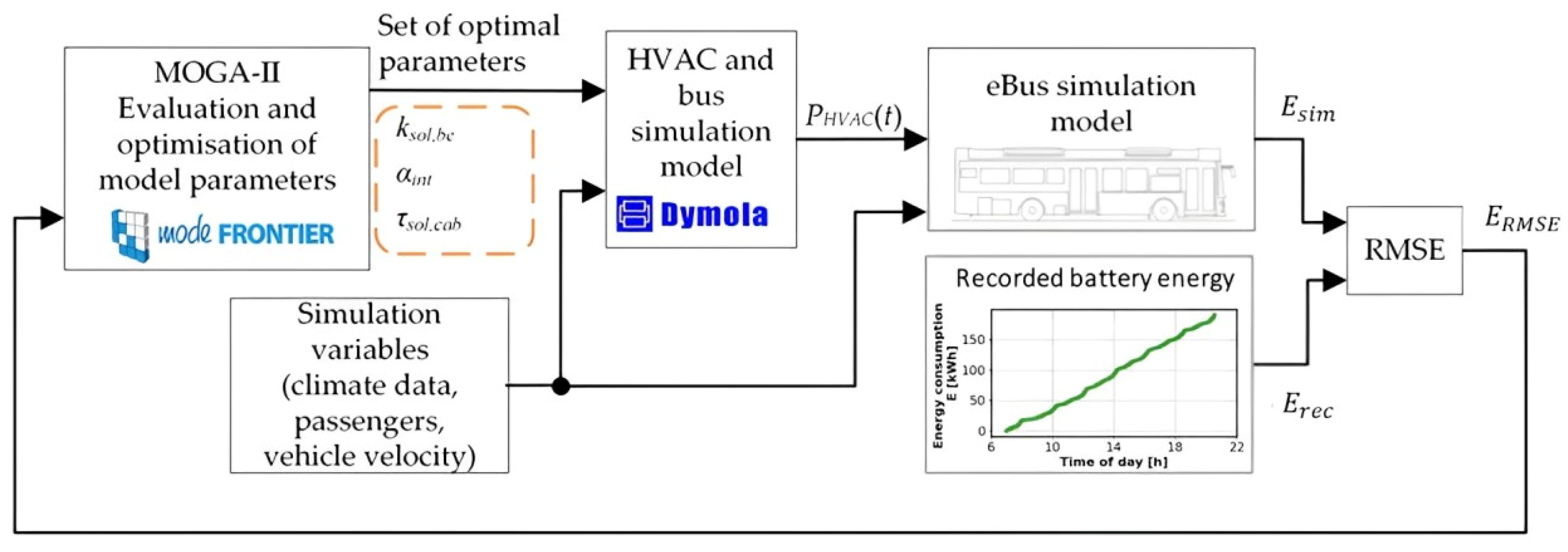
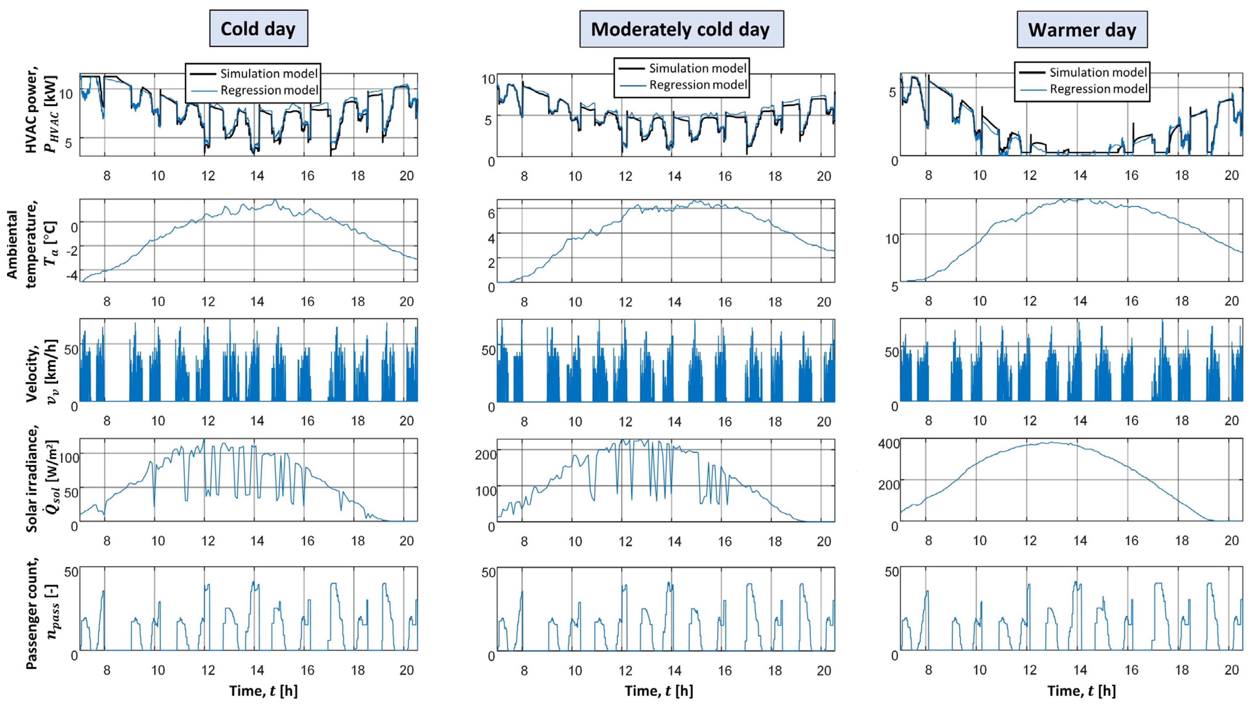
5.2. HVAC Trip-Based System Model

The HVAC power consumption regression model developed and indirectly experimentally validated within the physical e-bus model in Section 2 has a quadratic form gained by a feature selection method for four inputs: ambient temperature $T_a$, solar irradiation ${\dot{Q}}_{sol}$, ridership $n_{pass}$, and vehicle velocity $v_{veh}$ (see Equation (8)).

For integration into the trip-based data-driven model, the features of the HVAC model should be averaged on a per-trip basis. This modification is justified by two assumptions: (i) the ambient conditions, such as solar irradiation and temperature, remain approximately constant during a relatively short bus trip, and (ii) the velocity and ridership variables, which may significantly change during the trip, are of secondary influence on the HVAC consumption when compared to the influence of ambient condition variables. To further suppress the influence of velocity and ridership variations on mean value model accuracy, it is suitable to avoid the nonlinear terms of Equation (8), and thus in the model. It is shown that this intervention does not considerably deteriorate the accuracy of the physical model, and notably improves the accuracy of the mean value model, which is formulated as follows:

$$P_{HVAC}={\beta }_0+{\beta }_1{\overline{T}}_a+{\beta }_2{\overline{\dot{Q}}}_{sol}+{\beta }_3{\overline{n}}_{pass}+{\beta }_4{\mu }_v,$$

(12)

where the mean predictor variables are calculated over the trip, i.e., the driving cycle. The HVAC energy consumption per trip is then determined as follows:

$$E_{HVAC}=t_{trip}{P}_{HVAC},$$

(13)

where $t_{trip}$ is the trip duration.

The mean value HVAC model (12) and (13) was tested against the original model (8) by using the five-fold cross-validation method illustrated in Figure 14. The corresponding $R_{val}^2$ value was 0.999 and an ${RMSE}_{val}$ was only 0.128 kWh. This confirms that the mean value HVAC system model can be used with a negligible loss of accuracy.

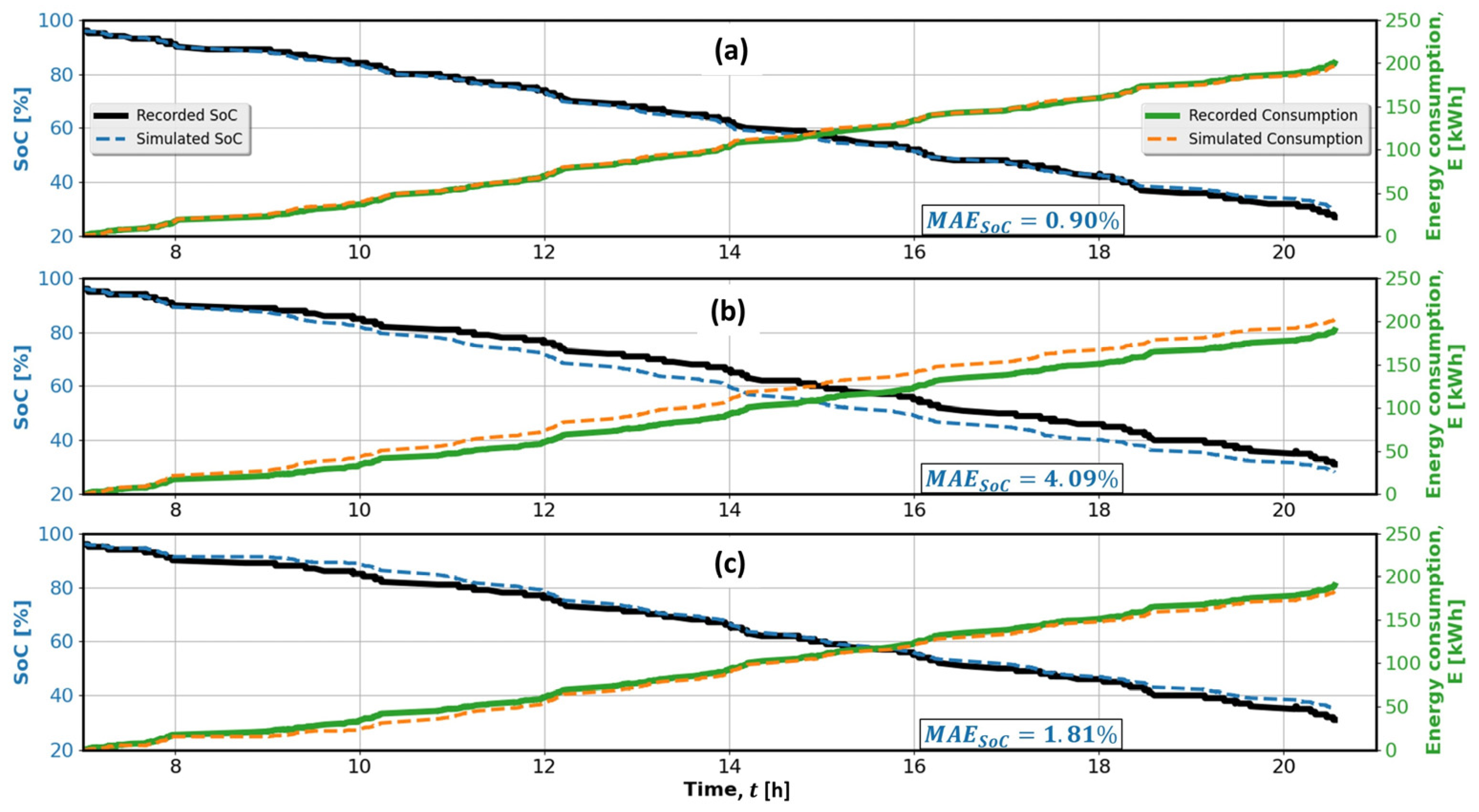
5.3. Overall E-Bus Model

The overall e-bus regression model integrates the powertrain and HVAC system submodels given by Equation (11) and Equations (12) and (13), respectively. It is represented by the expression given in the first row of

Table 7. Comparative analysis of the overall model with regression models used in literature.

	Regression Model
This study	$$\begin{gathered} E={\beta }_0{d}_{trip}+{\beta }_1{\mu }_{rg}{d}_{trip}+{\beta }_2{\mu }_{rg}^2{d}_{trip}+{\beta }_3{\sigma }_{rg}^2{d}_{trip}+{\beta }_4{\mu }_v{\overline{n}}_{pass}{d}_{trip}+ \\ {\beta }_5{t}_{trip}+{\beta }_6{\overline{T}}_a{t}_{trip}+{\beta }_7{\overline{\dot{Q}}}_{sol}{t}_{trip}+{\beta }_8{\overline{n}}_{pass}{t}_{trip}+{\beta }_9{\mu }_v{t}_{trip} \end{gathered}$$
Abdelaty et al. [18]	$$\begin{gathered} E={\beta }_0+{\beta }_{1}GR+{\beta }_2{D}_{agg}+{\beta }_3{R}_C+{\beta }_4{P}_{HVAC}+{\beta }_5{n}_{pass}+{\beta }_6{S}_D+{\beta }_7{\mu }_v+ \\ {\beta }_8{SoC}_{init}+{\beta }_9{d}_{trip} \end{gathered}$$
Vepsäläinen et al. [22]	$E={\beta }_0+{\beta }_1\left|20-T_{\mathrm{a}}\right|+{\beta }_2{P}_{dc}+{\beta }_3{S}_D+{\beta }_4{D}_{agg}$
Pamula et al. [17]	$E={\beta }_0{d}_n+{\beta }_1\mathsf{\Delta }t+{\beta }_2\mathsf{\Delta }h+{\beta }_{3}w$
Pamula et al. [19]	$E={\beta }_0{d}_n+{\beta }_1\mathsf{\Delta }t+{\beta }_2\mathsf{\Delta }h+{\beta }_{3}w+{\beta }_{4}tph$
Vehviläinen et al. [21]	$E=\left\{\begin{array}{c}{\beta }_0{T}_a^3+{\beta }_1{T}_a^2+{\beta }_2{T}_{\mathrm{a}}, if T_{\mathrm{a}}\ge 0°C\\ {\beta }_3{T}_{\mathrm{a}}, if T_{\mathrm{a}}<0°C\end{array}\right.$
Bie et al. [31]	$E={\beta }_0{SoC}_{init}+{\beta }_1{t}_{trip}+{\beta }_2{T}_a$
Xing et al. [23]	$E={\beta }_0+{\beta }_1\ln \left(\frac{1-{SoC}_{init}}{100}\right)+{\beta }_2{t}_{trip}+{\beta }_3{\mu }_v^2+{\beta }_4{\mu }_v+{\beta }_5{t}_a^2+{\beta }_6{t}_a$

$GR$ —road grade; $D_{agg}$ —driving aggressiveness; $R_C$ —road condition; $P_{HVAC}$ —power of the HVAC system; $S_D$ —stops density per km; $T_o$ —optimal operating temperature; $P_{dc}$ —DC converter power; $d_n$ —distance between stops; $\mathsf{\Delta }t$ —travel time between stops; $\Delta h$ —elevation difference between stops; $w$ —weather code; $tph$ —hour code; $t_a$ —operation time of the AC system of each trip.

and compared with existing models from the literature, listed in the remaining rows of Table 7. This comparison reveals that, although it includes similar features overall, the proposed model is generally richer than the existing individual models in terms of the number of features and nonlinearities accounted for (in terms of interactions). By relying solely on readily available and objective features, the model avoids subjective variables such as driving aggressiveness or road conditions, which could introduce bias and necessitate city-specific adjustments, potentially leading to overfitting. Being validated across diverse scenarios, including varying route profiles and traffic patterns, the model distinguishes itself by demonstrating robustness and broad applicability in diverse operational environments.

6. Analysis of Model Residuals

A practical analysis of model residuals was carried out separately for powertrain and HVAC models, as well as for the full vehicle model. The analysis results relate to the validation dataset aggregated from individual subsets #1–#5 (Figure 14).

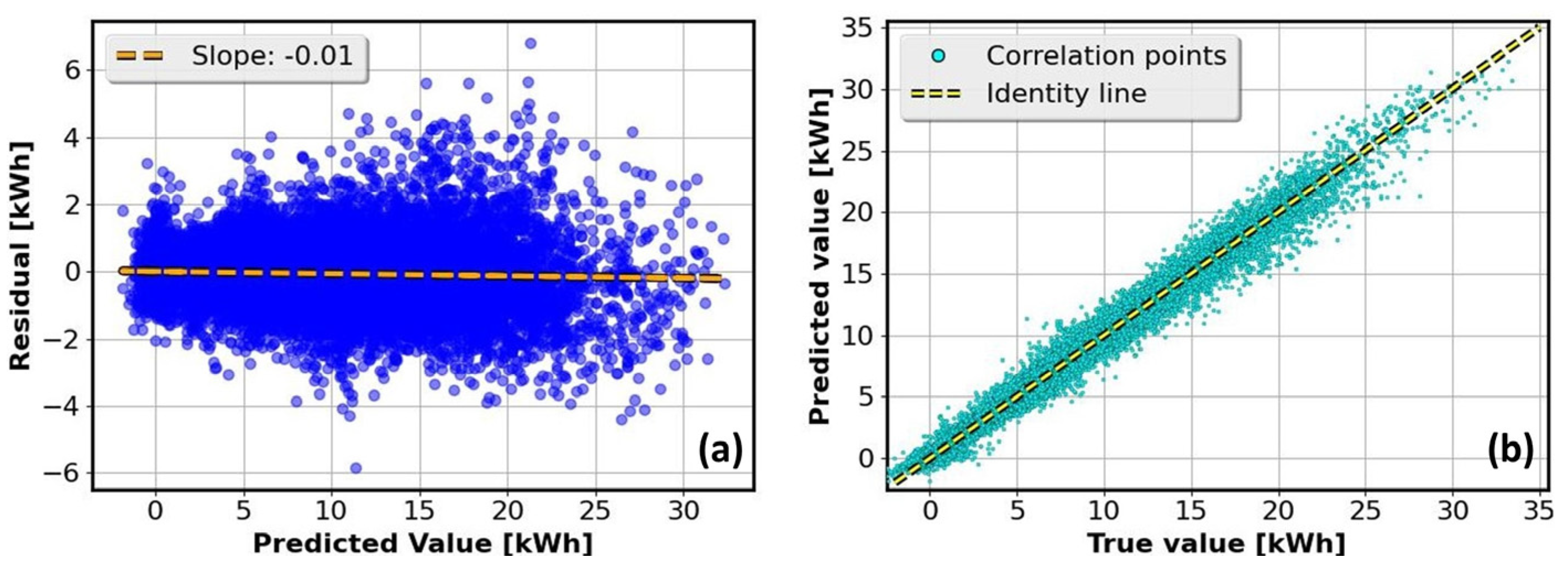
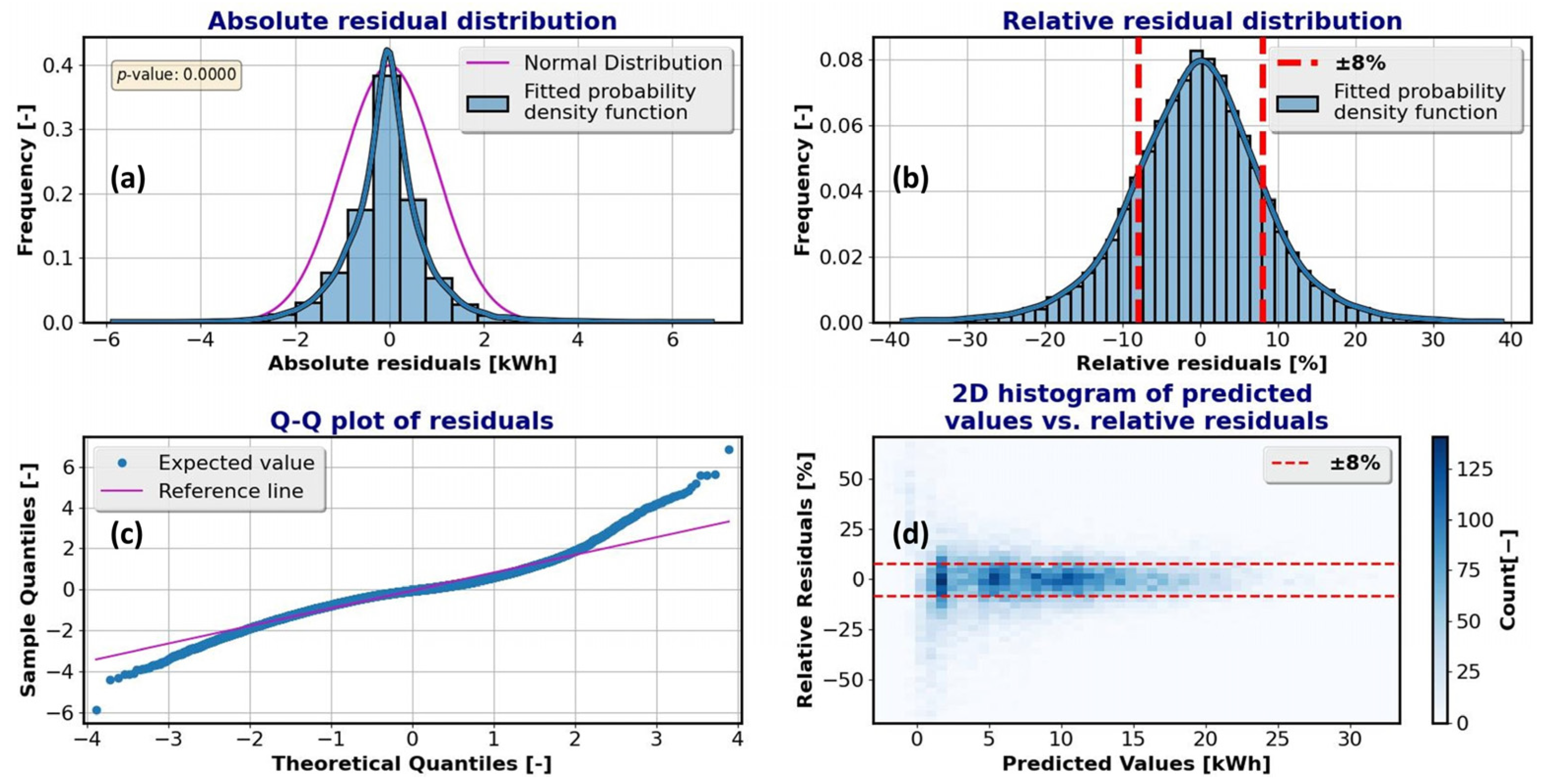
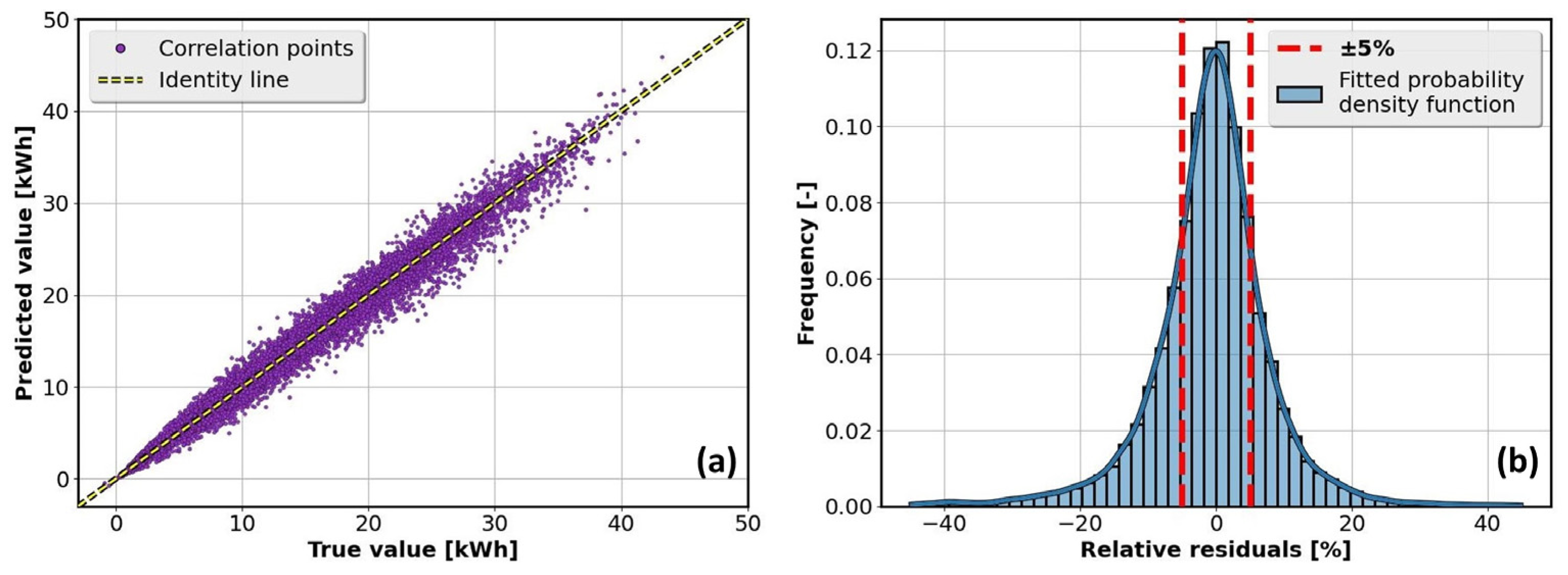
6.1. Powertrain Model

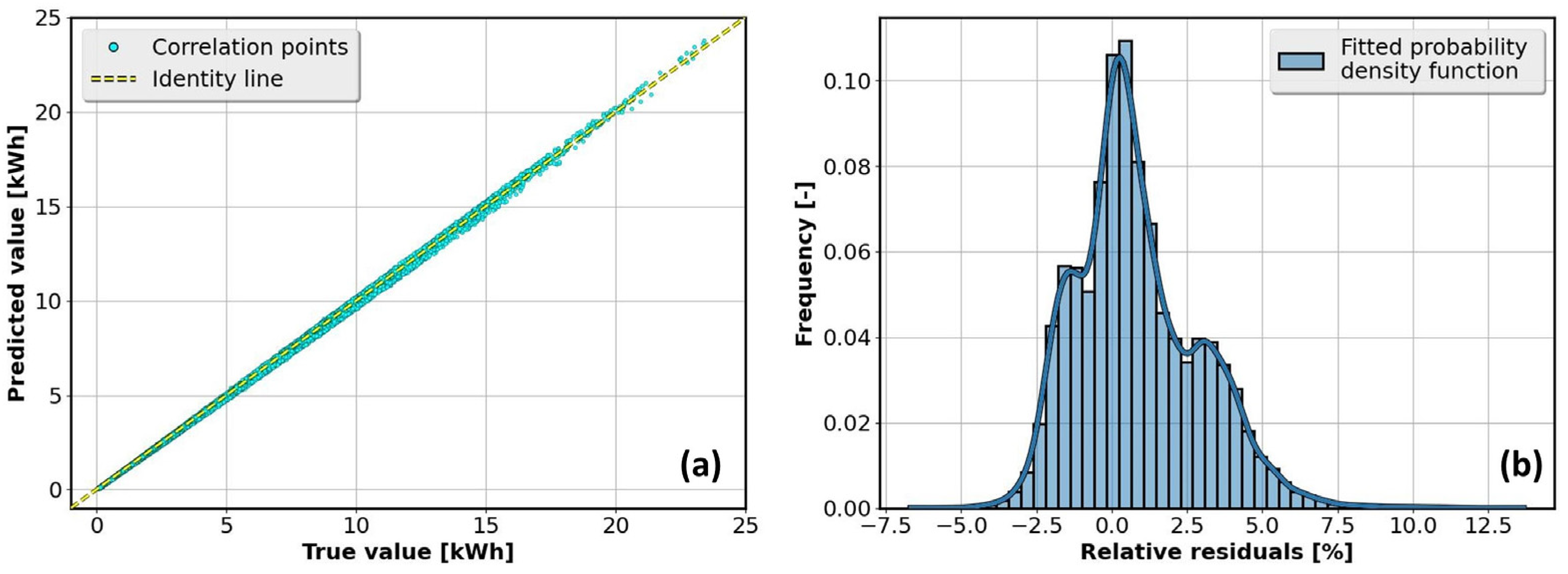
An essential step in evaluating regression models involves examining the spread of residuals against the predicted values, which should be distributed around a horizontal zero-value line without forming any distinct patterns [32]. The residual plot of the powertrain quadratic regression model from Table 3 is shown in Figure 19a. It indicates a slight slope of −0.015 kWh/kWh around the zero-value line, thus confirming the model consistency. Figure 19b shows that the model predictions scatter closely around the ideal identity line.

The normality of residuals is another model assessment criterion. Figure 20a demonstrates that, despite the p-value being lower than the normality threshold of 0.05, the residuals exhibit an unbiased, symmetric distribution resembling the normal distribution. The distribution of relative residuals, shown in Figure 20b, indicates that a great majority of relative residuals (90% of them, see

Table 8. Characterization of the absolute (Abs.) and relative (Rel.) residual distributions of the powertrain model.

	Mean	Std.	1%	5%	10%	15%	25%	50%	75%	85%	90%	95%	99%
Abs. [kWh]	−0.06	0.85	−2.31	−1.43	−1.02	−0.78	−0.47	−0.06	0.31	0.62	0.87	1.35	2.56
Rel. [%]	−0.50	6.93	−18.70	−11.51	−8.52	−6.75	−4.43	−0.45	3.46	5.87	7.65	10.72	17.83

) fall below the margin of 8%. The Q–Q plot in Figure 20c provides further illustration of the residual distribution normality by plotting the residuals in a manner that should form a straight line if they are normally distributed. Figure 20d shows a heat plot of the residual versus true value. It reveals that the higher relative residuals are associated with lower predicted values, which is apparently due to the nature of relative residual calculation that tends to be more sensitive to smaller values. Table 8 provides a summarized residual statistics.

6.2. HVAC Model

Figure 21 shows the main residual plots of the HVAC model given by Equations (12) and (13), while the corresponding statistics are given in

Table 9. Characterization of absolute (Abs.) and relative (Rel.) residual distributions for HVAC model.

	Mean	Std.	1%	5%	10%	15%	25%	50%	75%	85%	90%	95%	99%
Abs. [kWh]	0.02	0.11	−0.25	−0.16	−0.09	−0.05	−0.02	0.01	0.06	0.11	0.16	0.25	0.37
Rel. [%]	0.85	2.05	−2.86	−2.05	−1.64	−1.29	−0.51	0.52	2.09	3.19	3.74	4.48	6.28

. Ninety percent of residuals fall below the absolute and relative margins of 0.16 kWh or 3.74%, respectively, which confirms the good modeling accuracy.

6.3. Overall Model

Figure 22 shows the residual analysis results for the overall e-bus model (both powertrain and HVAC models). The relative residual distribution was narrower than for the powertrain model (cf. Figure 20b and Figure 22b) due to the accuracy contribution of the HVAC submodel. Consequently, the score $R_{val}^2$ of the full model (when validated on the aggregate dataset) increased from the powertrain model validation value of 0.9756 (Table 3) to 0.9812.

Table 10. Computational time comparison for physical and regression models (for 20.285 trips).

Type of Model	$\mathbf{Total} \mathbf{Elapsed} \mathbf{Time}, {\mathit{T}}_{\mathit{e}\mathit{x}\mathit{e}\mathit{c}}$ *	Average Execution Time per Trip
Physical model	2920 s	0.14 s
Regression model	1.5 ms	74 ns

* The computations were performed on a Dell G5 15 Laptop (Dell, Round Rock, TX, USA), equipped with an Intel(R) Core(TM) i7-10750H CPU @ 2.60 GHz, 16.0 GB RAM (Intel, Santa Clara, CA, USA), running on a 64-bit Windows 11 Home operating system, utilizing Python version 3.10 and TensorFlow-gpu version 2.10.0, with an Intel(R) UHD Graphics GPU.

shows a comparison of the execution time for routines that predict energy consumption across 20,285 trips using the regression model and its physical counterpart. The total execution time when using the physical model is 2920 s, which gives the average value of 0.14 s per trip. In contrast, the regression model requires a total execution time of only 1.5 milliseconds, averaging about 74 nanoseconds per trip, which is approximately 2,000,000 times faster than the physical model. Accordingly, the regression model can conveniently be used in large-scale electrification planning simulation and optimization studies to facilitate assessment and decision-making processes for numerous scenarios.

7. Conclusions

A method for predicting the battery energy consumption of electric city buses (e-buses) using a trip-based data-driven regression model was proposed in the paper. The method was designed to strike a balance between model accuracy, computational efficiency, and generalization capabilities. The key findings of the presented study are as follows:

• A backward-looking physical model of a 12 m electric city bus was developed, with an emphasis on the heating, ventilation, and air conditioning (HVAC) system submodel. For the sake of e-bus model implementation simplicity and numerical efficiency, a quadratic regression HVAC model was set up and its parameters were optimized based on the responses of a physical HVAC model developed in Dymola 2018 FD01. The developed e-bus model was successfully validated with respect to several recorded datasets not used in the stage of model parameterization;
• The emphasis was then placed on the data-driven model, derived from simulations of the physical model under a wide set of traffic, road, and ambient conditions. The model relies on typically available trip-related data, as opposed to the physical model, which requires high-sampling-rate driving cycle data. It consists of independent powertrain and HVAC submodels to resemble the structure of the physical model. For the powertrain, a feature selection method was used to find an optimal quadratic regression model for the specific energy consumption (in kWh/km), where the selected features include the mean road grade and its square, the road grade standard deviation square, and the product of mean velocity and ridership. The model performance (characterized by the validation R² value of 0.975) is comparable to more complex methods such as neural networks and gradient boosting but with the added advantage of greater simplicity and generalization (i.e., robustness);
• An exploration into a better quantized, station-to-station segment modeling approach did not enhance the modeling accuracy when compared to the trip-based approach. On the other hand, the modeling accuracy was found to notably grow when extending the feature set with vehicle acceleration and deceleration features, thus underscoring the significance of including a broader set of relevant features as opposed to making the quantization of the basic feature set denser. However, the vehicle acceleration features are usually unavailable in real city bus transport systems. Thus, the basic, narrow feature set-based quadratic regression model is generally recommended for applications due to low data demands, simplicity, and favorable accuracy;
• The original HVAC system model with four inputs (ambient temperature, solar irradiance, vehicle velocity, and ridership) was reformulated to have (i) a mean value form to be applicable to trip-based inputs of the data-driven model and (ii) a linear structure to suppress the influence of velocity and ridership variation on mean value modeling accuracy;
• When validating the overall model on an aggregated dataset, it registered a notable R² score of 0.981. It executes approximately 1,900,000 times faster than the physical model, thereby offering both accurate energy consumption predictions and computational efficiency for large-scale simulation and optimization studies of city bus fleet electrification planning;
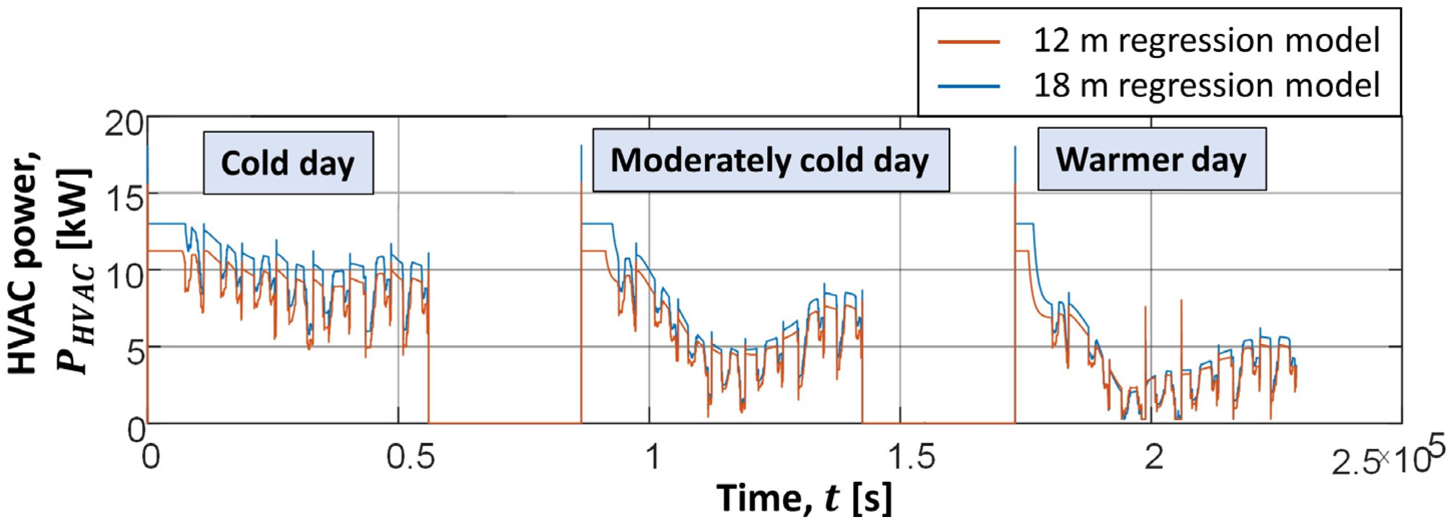
• Although the proposed modeling approach was demonstrated on a 12 m fully electric city bus and A/C operating mode, it can be readily applied to other sizes (e.g., 18 m) and types of city buses (e.g., HEV, PHEV, and H2 buses), as well as for other operating conditions (e.g., heat pump mode).

References

1. Miles, J.M.; Potter, S. Developing a Viable Electric Bus Service: The Milton Keynes Demonstration Project. Res. Transp. Econ. 2014, 48, 357–363. [Google Scholar] [CrossRef]
2. Li, J. Battery-Electric Transit Bus Developments and Operations: A Review. Int. J. Sustain. Transp. 2014, 10, 157–169. [Google Scholar] [CrossRef]
3. Kang, J.; Huang, X.; Maharjan, S.; Zhang, Y.; Hossain, E. Enabling Localized Peer-to-Peer Electricity Trading Among Plug-in Hybrid Electric Vehicles Using Consortium Blockchains. IEEE Trans. Ind. Inform. 2017, 13, 3154–3164. [Google Scholar] [CrossRef]
4. Deur, J.; Cvok, I.; Ratković, I.; Topić, J.; Soldo, J.; Maletić, F. Backward-looking Modelling of a Fully Electric City Bus with Emphasis on Cabin Heating and Cooling Subsystem. In Proceedings of the 18th Conference on Sustainable Development of Energy, Water and Environment Systems (SDEWES), Dubrovnik, Croatia, 24–29 September 2023. [Google Scholar]
5. Tim, J.; Hunter, C.D.; Macht, G.A. Quantifying the Impact of Traffic on Electric Vehicle Efficiency. World Electr. Veh. J. 2022, 13, 15. [Google Scholar] [CrossRef]
6. Perumal, S.S.G.; Lusby, R.M.; Larsen, J. Electric Bus Planning & Scheduling: A Review of Related Problems and Methodologies. 2022. Available online: https://ideas.repec.org/a/eee/ejores/v301y2022i2p395-413.html (accessed on 9 December 2023).
7. Teng, J.; Chen, T.; Fan, W. Integrated Approach to Vehicle Scheduling and Bus Timetabling for an Electric Bus Line. J. Transp. Eng. Part A Syst. 2019, 146, 04019073. [Google Scholar] [CrossRef]
8. Matković, D.; Topić, J.; Škugor, B.; Deur, J. Search Space Reduction-Supported Multi-objective Optimization of Charging System Configuration for Electrified City Bus Transport System. In Proceedings of the 17th Conference on Sustainable Development of Energy, Water and Environment Systems (SDEWES), Paphos, Cyprus, 6–10 November 2022. [Google Scholar]
9. An, K. Battery Electric Bus Infrastructure Planning under Demand Uncertainty. Transp. Res. Part C Emerg. Technol. 2020, 111, 572–587. [Google Scholar] [CrossRef]
10. Zhao, L.; Alipour-Fanid, A.; Slawski, M.; Zeng, K. Prediction-Time Efficient Classification Using Feature Computational Dependencies. In Proceedings of the 24th ACM SIGKDD International Conference on Knowledge Discovery & Data Mining, London, UK, 19–23 August 2018. [Google Scholar] [CrossRef]
11. Jahic, A.; Eskander, M.; Avdevicius, E.; Schulz, D. Energy Consumption of Battery- Electric Buses: Review of Influential Parameters and Modelling Approaches. B&H Electr. Eng. 2023, 17, 7–17. [Google Scholar] [CrossRef]
12. Perugu, H.; Collier, S.; Tan, Y.; Yoon, S.; Herner, J. Characterization of Battery Electric Transit Bus Energy Consumption by Temporal and Speed Variation. Energy 2023, 263, 125914. [Google Scholar] [CrossRef]
13. Dabčević, Z.; Škugor, B.; Topić, J.; Deur, J. Synthesis of Driving Cycles Based on Low-Sampling-Rate Vehicle-Tracking Data and Markov Chain Methodology. Energies 2022, 15, 4108. [Google Scholar] [CrossRef]
14. Al-Ogaili, A.S.; Ramasamy, A.K.; Tengku Hashim, T.J.; Al-Masri, A.N.; Hoon, Y.; Jebur, M.N.; Verayiah, R.; Marsadek, M. Estimation of the Energy Consumption of Battery Driven Electric Buses by Integrating Digital Elevation and Longitudinal Dynamic Models: Malaysia as a Case Study. Appl. Energy 2020, 280, 115873. [Google Scholar] [CrossRef]
15. Lin, K.-C.; Lin, C.-H.; Ying, J.J.-C. Construction of Analytical Models for Driving Energy Consumption of Electric Buses through Machine Learning. Appl. Sci. 2020, 10, 6088. [Google Scholar] [CrossRef]
16. Ji, J.; Bie, Y.; Zeng, Z.; Wang, L. Trip Energy Consumption Estimation for Electric Buses. Commun. Transp. Res. 2022, 2, 100069. [Google Scholar] [CrossRef]
17. Pamuła, T.; Pamuła, W. Estimation of the Energy Consumption of Battery Electric Buses for Public Transport Networks Using Real-World Data and Deep Learning. Energies 2020, 13, 2340. [Google Scholar] [CrossRef]
18. Abdelaty, H.; Mohamed, M. A Prediction Model for Battery Electric Bus Energy Consumption in Transit. Energies 2021, 14, 2824. [Google Scholar] [CrossRef]
19. Pamuła, T.; Pamuła, D. Prediction of Electric Buses Energy Consumption from Trip Parameters Using Deep Learning. Energies 2022, 15, 1747. [Google Scholar] [CrossRef]
20. Qin, W.; Wang, L.; Liu, Y.; Xu, C. Energy Consumption Estimation of the Electric Bus Based on Grey Wolf Optimization Algorithm and Support Vector Machine Regression. Sustainability 2021, 13, 4689. [Google Scholar] [CrossRef]
21. Vehviläinen, M.; Lavikka, R.; Rantala, S.; Paakkinen, M.; Laurila, J.; Vainio, T. Setting Up and Operating Electric City Buses in Harsh Winter Conditions. Appl. Sci. 2022, 12, 2762. [Google Scholar] [CrossRef]
22. Vepsäläinen, J.; Ritari, A.; Lajunen, A.; Kivekäs, K.; Tammi, K. Energy Uncertainty Analysis of Electric Buses. Energies 2018, 11, 3267. [Google Scholar] [CrossRef]
23. Xing, Y.; Li, Y.; Liu, W.; Li, W.; Meng, L.-X. Operation Energy Consumption Estimation Method of Electric Bus Based on CNN Time Series Prediction. Math. Probl. Eng. 2022, 2022, 6904387. [Google Scholar] [CrossRef]
24. Guzzella, L.; Sciarretta, A. Vehicle Propulsion Systems; Springer: Berlin/Heidelberg, Germany, 2013. [Google Scholar] [CrossRef]
25. André, D.; Meiler, M.; Steiner, K.; Walz, H.; Soczka-Guth, T.; Sauer, D.U. Characterization of High-Power Lithium-Ion Batteries by Electrochemical Impedance Spectroscopy. II: Modelling. J. Power Sources 2011, 196, 5349–5356. [Google Scholar] [CrossRef]
26. Göhlich, D.; Fay, T.-A.; Jefferies, D.; Lauth, E.; Kunith, A.; Zhang, X. Design of urban electric bus systems. Des. Sci. 2018, 4, e15. [Google Scholar] [CrossRef]
27. Zhang, T.; Gao, C.; Gao, Q.; Wang, G.; Liu, M.; Guo, Y.; Xiao, C.; Yan, Y.Y. Status and development of electric vehicle integrated thermal management from BTM to HVAC. Appl. Therm. Eng. 2015, 88, 398–409. [Google Scholar] [CrossRef]
28. Freedman, D.; Pisani, R.; Purves, R. Statistics, 3rd ed.; W.W. Norton: New York, NY, USA, 1998. [Google Scholar]
29. Seber, G.A.F.; Lee, A.J. Linear Regression Analysis, 2nd ed.; John Wiley & Sons, Inc.: Hoboken, NJ, USA, 2003. [Google Scholar]
30. Stańczyk, U.; Jain, L. Feature Selection for Data and Pattern Recognition; Springer: Berlin/Heidelberg, Germany, 2016. [Google Scholar]
31. Bie, Y.; Jinhua, J.; Wang, X.; Qu, X. Optimization of electric bus scheduling considering stochastic volatilities in trip travel time and energy consumption. Comput. Aided Civ. Infrastruct. Eng. 2021, 36, 1530–1548. [Google Scholar] [CrossRef]
32. Dodge, Y. Analysis of Residuals, 1st ed.; Springer: New York, NY, USA, 2008. [Google Scholar]
Figure 1. Recorded city bus driving cycle time profile data: vehicle velocity and distance traveled (a), ridership (b), and ambient temperature and solar irradiance (c).
Energies 17 00911 g001
Figure 2. Reconstructed road altitude (a) and road slope profiles (b) with respect to distance traveled.
Energies 17 00911 g002
Figure 3. Time profiles of battery S o C and cumulative battery energy consumption.
Energies 17 00911 g003
Figure 4. Normalized efficiency map and maximum torque characteristics of e-machine.
Energies 17 00911 g004
Figure 5. Battery equivalent circuit (a) and S o C dependencies of the open-circuit voltage and internal battery resistance for considered LFP battery (b).
Energies 17 00911 g005
Figure 6. Illustration of HVAC system energy consumption model.
Energies 17 00911 g006
Figure 7. E-bus cabin thermal model implemented in Dymola 2018 FD01.
Energies 17 00911 g007
Figure 8. Block diagram of optimization setup used to determine unknown parameters of e-bus cabin thermal model.
Energies 17 00911 g008
Figure 9. The response of recorded e-bus model variables for the dataset used in model training and corresponding simulation responses of S o C , energy consumption, and HVAC power.
Energies 17 00911 g009
Figure 10. E-bus model validation for first (a) and second validation dataset (b), as well as for second validation dataset but with simulated A/C system switched off from 7 a.m. to 10 a.m. (c).
Energies 17 00911 g010
Figure 11. Simulated vs. recorded values of specific energy consumption (a) and simulated specific energy consumption vs. average vehicle velocity (b).
Energies 17 00911 g011
Figure 12. Illustration of data collection framework.
Energies 17 00911 g012
Figure 13. Distributions of main features of standard, modified, and aggregate driving cycle sets and the corresponding distribution of powertrain energy consumption (PDF stands for probability density function).
Energies 17 00911 g013
Figure 14. Schematic representation of the model cross-validation strategy.
Energies 17 00911 g014
Figure 15. Illustration of LASSO feature selection technique in particular case of n = 11 predictor variables and m = 77 features of energy consumption quadratic regression model.
Energies 17 00911 g015
Figure 16. Feature importance distribution as determined by Random forest importance analysis.
Energies 17 00911 g016
Figure 17. Comparative plots of aggregate R2 values for the LASSO and Random forest importance feature selection methods.
Energies 17 00911 g017
Figure 18. Validation results for the best subset method in terms of R² metrics vs. number of predictor variables (a), and RMSE metrics vs. number of predictor variables (b).
Energies 17 00911 g018
Figure 19. Powertrain model residuals plotted vs. predicted values (a) and model predicted vs. true value plot (b).
Energies 17 00911 g019
Figure 20. Characteristic powertrain model residual plots.
Energies 17 00911 g020
Figure 21. The HVAC model’s predicted vs. true value plot (a) and corresponding relative residual distribution plot (b).
Energies 17 00911 g021
Figure 22. The overall e-bus model’s predicted vs. true value plot (a) and corresponding relative residuals distribution plot (b).
Energies 17 00911 g022