Data-Driven Modeling of Appliance Energy Usage

Abstract

Due to the transition toward the Internet of Everything (IOE), the prediction of energy consumed by household appliances has become a progressively more difficult topic to model. Even with advancements in data analytics and machine learning, several challenges remain to be addressed. Therefore, providing highly accurate and optimized models has become the primary research goal of many studies. This paper analyzes appliance energy consumption through a variety of machine learning-based strategies. Utilizing data recorded from a single-family home, input variables comprised internal temperatures and humidities, lighting consumption, and outdoor conditions including wind speed, visibility, and pressure. Various models were trained and evaluated: (a) multiple linear regression, (b) support vector regression, (c) random forest, (d) gradient boosting, (e) xgboost, and (f) the extra trees regressor. Both feature engineering and hyperparameter tuning methodologies were applied to not only extend existing features but also create new ones that provided improved model performance across all metrics: root mean square error (RMSE), coefficient of determination (R²), mean absolute error (MAE), and mean absolute percentage error (MAPE). The best model (extra trees) was able to explain 99% of the variance in the training set and 66% in the testing set when using all the predictors. The results were compared with those obtained using a similar methodology. The objective of performing these actions was to show a unique perspective in simulating building performance through data-driven models, identifying how to maximize predictive performance through the use of machine learning-based strategies, as well as understanding the potential benefits of utilizing different models.

1. Introduction

In the energy industry, specific simulation tools are frequently used to study and predict building energy consumption. Examples of these tools include DOE-2, Energy Plus, ESP-r, and DeST. Although these tools can accurately predict building loads and energy use, unlike machine learning models, they frequently require the physical and geometric properties of the buildings being analyzed. Using machine learning can simplify the data requirements needed to perform a specific analysis. Furthermore, the physical models can vary depending on the software used for the analysis [1]. With the recent rise of artificial intelligence and machine learning, more work is being performed to integrate machine learning techniques into the field. This can be identified in numerous studies [2,3,4,5,6], giving researchers the opportunity to utilize machine learning tools to study the effect of numerous building parameters on energy-based outputs, making the procedure more efficient if a database of similar structure is available.

For this specific case, focus is placed on “Data driven prediction models of energy use of appliances in a low-energy house” by Candanedo, L.M.; Feldheim, V.; and Deramaix, D. [2]. With the emphasis being model improvement, work is performed on applying methodologies including feature engineering [7,8,9,10] that leverages data to create new variables that are not found in the original dataset, with the goal of simplifying and speeding up data transformations while also improving model accuracy. Correlation analyses [11,12,13] are utilized to identify how well parameters correlate with each other in order to determine whether certain variables have to be dropped or adapted to form stronger relationships within the dataset. Hyperparameter tuning [14,15,16,17,18] is utilized to test different hyperparameter configurations when training models, providing the optimized hyperparameter set that will maximize a model’s predictive accuracy. Six regression models were applied and tested; these included (a) multiple linear regression (LM), (b) support vector regression (SVR), (c) random forest (RF), (d) gradient boosting (GB), (e) xgboost (XGB), and (f) extra trees (ET). The first four models, (a)–(d), were utilized in the original analysis, and the goal was to use these same models again to prove the effectiveness of the methodologies mentioned above and how they alone can significantly improve model performance. Models (e)–(f), on the other hand, are more advanced machine learning algorithms, with the idea of fully maximizing performance to achieve the best possible results. Further details of these models are provided in Section 3.2.

To reiterate, the analysis deals with simulating aggregated appliance energy use utilizing machine learning algorithms. Therefore, we focused on machine learning applications for energy efficiency, appliance energy use, building loads, and building energy consumption, as well as general overviews on model optimization, in order to analyze how different approaches and strategies can be applied to predicting appliance energy use, including methods that can be used to improve performance.

“Accurate quantitative estimation of energy performance of residential buildings using statistical machine learning tools” [3] developed a machine learning framework to precisely quantify the energy efficiency of residential buildings, where the impact of eight input factors—relative compactness, surface area, wall area, roof area, overall height, orientation, glazing area, and glazing area distribution—on two key output variables, heating load (HL) and cooling load (CL), was investigated. In the study, classical linear regression and random forest were utilized to estimate HL and CL. Simulations were performed on 768 diverse residential buildings and compared to results from Ecotect, a tool specifically used for building and environment simulations. The results supported the practicality of using machine learning tools to estimate building parameters as a precise and straightforward approach.

“Gradient boosting machine for modeling the energy consumption of commercial buildings” [5] focuses specifically on accurate savings estimations paired with advanced metering infrastructure (AMI) data, in order to evaluate energy efficiency applications including demand response, and heating, ventilation, and air conditioning (HVAC) optimization. Gradient boosting was applied to work on an energy consumption baseline modeling method. To assess the performance, a large dataset of 410 commercial buildings was included in the testing procedure. The results demonstrated that using GB improved the machine learning metrics R-squared and RMSE, in more than 80 percent of the cases, when compared to an industry-standard model that was created using piecewise linear regression.

When reviewing the overall appearance of machine learning in energy efficiency, it can be seen that various models such as polynomial regression [19], support vector machines (SVM) [4,20], artificial neural networks (ANNs) [21,22], and decision trees [5,6] have been utilized to predict specific variables within the energy efficiency field. Machine learning tools have also been explicitly used in predicting appliance energy use in other studies. Moldovan and Slowik [23] used multi-objective binary gray wolf optimization, employing the algorithms random forest, extra trees, decision tree, and K-nearest neighbor to predict the energy consumed by household appliances. Lentzas and Vrakas [24] applied a decision table, random forest, naive Bayes, multilayer perceptron (MLP), and a deep neural network (Deep NN) to the UK-DALE dataset, a well-known dataset for non-intrusive load monitoring (NILM), in order to predict appliance energy use as a method for identifying the occupancy of residents in households. Priyadarshini et al. [25] focused on monitoring energy consumption in smart homes by deploying decision trees (DTs), random forest (RF), extreme gradient boosting (XGB), and K-nearest neighbor (KNN) and proposing a DT-RF-XGB ensemble model that was compared to the baseline algorithms. Ma et al. [26] employed hybrid deep learning models to enhance the energy efficiency of HVAC systems in smart buildings. Their optimization focused on factors such as power loss, price management, and reactive power. Examples of these models included long short-term memory (LSTM), gated recurrent unit (GRU), and Drop-CRU. Wang et al. [27] used machine learning in the context of energy forecasting to reduce the overconsumption of household power. Deep learning with a metaheuristic-based algorithm was proposed to address the constraints and consumption of HVAC units. Perwez et al. [28] integrated spatial and synthetic techniques in the context of a novel hybrid model in order to investigate multiple building-orientated elements, including building system stock dynamics and HVAC systems.

The rest of this paper includes four other sections. Section 2 provides an in-depth description of the data and a look into the correlation studies and feature engineering that were performed on the original dataset. Section 3 breaks down the results, including the models that were used and why, training and testing procedures that were applied to the models, and metrics that were utilized to understand the performance of each model. Section 4 discusses the results in order to analyze how each model performed relative to the others and the original analysis. Section 5 provides concluding thoughts and suggestions for future work that could help contribute to this analysis and prior research performed in this area.

2. Materials and Methods

Although the data were collected from the UC Irvine (UCI) Machine Learning Repository, a brief description of how the data were recorded is provided as a means to include both context and reasoning for utilizing certain methodologies.

As mentioned in the introduction, various features were monitored within a single-family home. Aggregated appliance energy use included a variety of residential devices: fridge/freezer, washing machine, dryer, internet router, induction cooktop, microwave, oven, dishwasher, electrical blinds, TV, laptop, printer, alarm clock, lamps, and radio. The corresponding information was recorded with an internet-connected energy monitoring system. The indoor temperature and humidity conditions were monitored with a wireless sensor network. The sensors, used to record temperature and humidity, were placed on all floors in different rooms of the house, including the laundry room, kitchen, living room, office, bedrooms, and bathrooms.

The overall goal was to predict aggregated appliance energy use, which in this case was continuous numerical data, recorded in watt-hours (Wh) and jotted every 10 min. Lighting consumption was incorporated because it proved to be a reliable predictor of room occupancy when coupled with relative humidity measurements. All data modeling and preprocessing were performed in Python, more specifically Google Colab [29]. The time span of the dataset was 137 days (4.5 months). The packages utilized in this analysis included NumPy [30], Matplotlib [31], Pandas [32], and Scikit-Learn [33]. For outdoor variables, data were monitored using a nearby airport weather station. Features that were monitored included temperature, pressure, humidity, wind speed, visibility, and dewpoint temperature. This was done in order to evaluate the impact of outdoor conditions on appliance energy use. Any data that were not collected in 10 min intervals were averaged across 10 min periods in order for merging to be successful.

Table 1. Data variables and their corresponding units.

Variables	Units
Appliance energy consumption	Wh
Light energy consumption	Wh
T1-T9, Indoor temperatures	°C
RH1-RH9, Indoor humidities	%
To, Temperature outside	°C
Pressure	mm Hg
RHo, Humidity outside	%
Wind speed	m/s
Visibility *	km
Tdewpoint	°C
Number of seconds from midnight (NSM)	s
Week status (weekend or weekday)	Categorical
Day of week	Categorical
Date time stamp *	year-month-day
	hour:min:s
Month	month
Day	day
Hour	h
Hour_sin, hour sine transformation	-
Hour_cos, hour cosine transformation	-
Season (autumn, winter, spring, or summer)	Categorical

* Any variable marked was either dropped from the analysis or not directly included.

provides the complete list of features for this dataset. Utilizing existing data, the original study also derived three supplementary variables: the number of seconds from midnight for each day (NSM), the categorization of the day as a weekend or workday, and the specific day of the week. As a final note, since there were not any issues with the overall data in terms of shape, formatting, significant outliers, null cells, or incorrect data types, additional data exploration beyond the correlation analysis and feature engineering conducted in Section 3.1 was not undertaken.

3. Results

3.1. Data Preprocessing

Two major data preprocessing techniques were utilized in order to improve overall model performance. These included correlation analysis and feature engineering. This was preferred over traditional approaches like principal component analysis (PCA) [34] or singular value decomposition (SVD) [35] due to the desire to study not only feature relationships, but also how features correlated with the target variable (appliances). Furthermore, by keeping the data as physical variables, the results can be more easily compared to other methodologies such as building models from DOE-2 or Energy Plus, versus transforming the data into a set of uncorrelated principal components. Correlation analysis was used to determine the relationship between multiple variables. By identifying the correlation between variables, it becomes possible to understand how they influence each other and how they might interact in the analysis. This can be useful in a number of ways, such as identifying and removing variables that show a lack of correlation with other features, as well as discovering unique relationships that are not necessarily intuitive on the surface when initially reviewing data. Feature engineering, on the other hand, was used to create new features from the existing ones. This helps to provide more relevant and useful information. In some cases, certain features can be transformed and normalized to a particular range, allowing for a possible reduction in data discontinuity. The impact of both methods for this analysis will be discussed further in the following subsections.

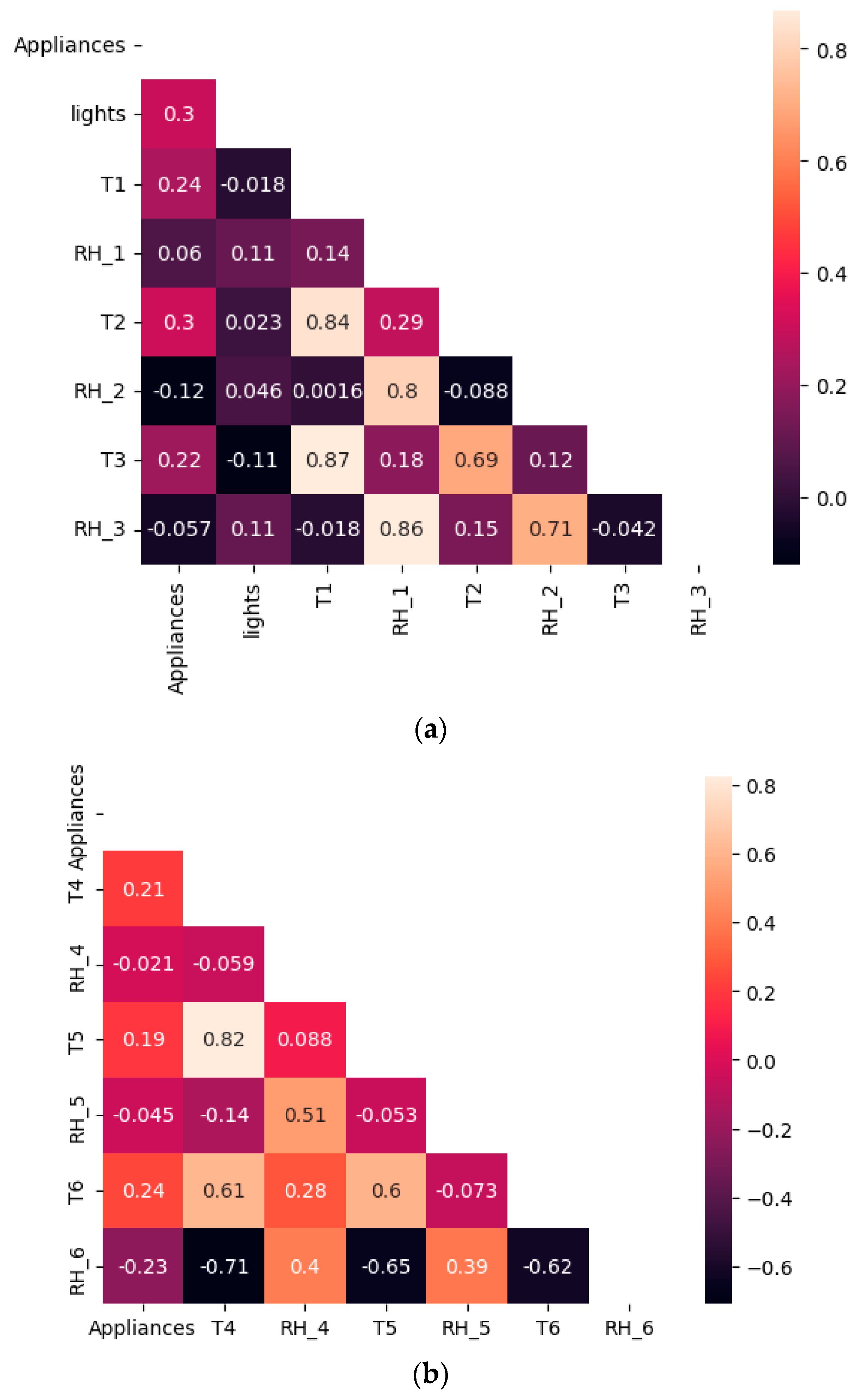
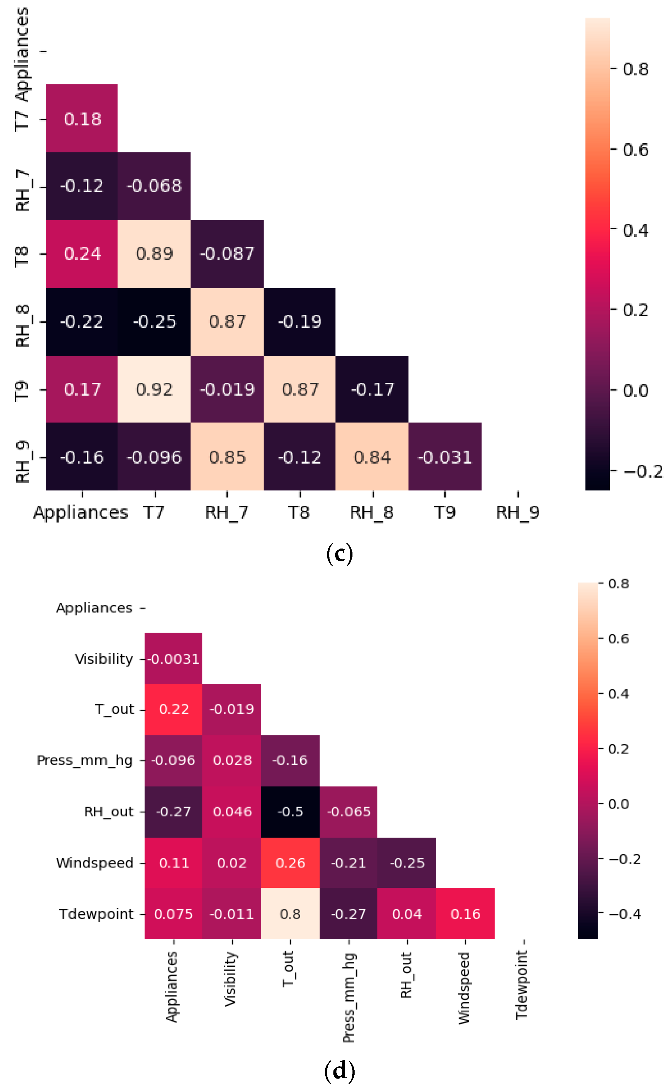
3.1.1. Correlation Analysis

The correlation analysis was executed using Spearman′s Rank [36], a coefficient that spans the range from −1 to +1. A coefficient of +1 signifies a perfect positive correlation, −1 denotes a perfect negative correlation, and 0 signifies a complete absence of any relationship. The equation is provided below, where d_i is the difference between the ranks of each observation and n is the number of observations. The ranking is achieved by giving the ranking of ‘1’ to the largest value in a variable, ‘2’ to the second largest, and so on.

$$\rho =1-\frac{6{\sum }_{i=1}^n{d}_i^2 }{n(n^2-1)}$$

(1)

As shown in Figure 1a, notable variables included lighting consumption and T2 at 0.3. Lighting and appliance energy use are both major sources of energy consumption, not only in households but in commercial buildings as well. Since T2 is the living room temperature, a living room is the most used room in a household; therefore, the temperature in a highly occupied room can heavily influence how people use appliances. For the remaining indoor temperatures, the correlations are all relatively high and positive. For Figure 1b, the correlations between appliance energy use and T4, T5, and T6 are 0.21, 0.19, and 0.24, respectively. For Figure 1c, T7, T8, and T9 have correlations of 0.18, 0.24, and 0.17 with appliance energy use. A positive correlation of 0.22 is seen between appliances and outdoor temperature. Wind speed also exhibited a positive correlation of 0.11 with appliances. Visibility was the only variable that showed little to no correlation with appliances (−0.0031); therefore, it was removed from the dataset.

3.1.2. Feature Engineering

As mentioned in the data section, the original paper generated three extra variables from the raw data: the number of seconds from midnight for each day (NSM), the categorization of the day as a weekend or workday, and the specific day of the week. In reviewing this, there was an opportunity to introduce a few additional variables using the date time stamp provided in the raw data. Since the time stamp was not integrated into the modeling, additional information can be extracted. Hour, month, and day features were created from the time stamp.

Using the monthly variable, seasonal categorical data were created (autumn, winter, spring, or summer) based on the corresponding month. Before modeling, the seasonal data were converted into numeric form using label encoding [37]. For this case, the data were converted into a number sequence: {0,1,2,3}, where 0 represents autumn, 1 represents winter, 2 represents spring, and 3 represents summer.

When reviewing the cyclical features (hour, month, and day), there was an opportunity for encoding using sine/cosine transformations [38]. These are performed to normalize the range and reduce the discontinuity in the data. In order to perform these transformations successfully, the feature has to be consistent, complete, and a repeated cycle. Therefore, both the month and day features were ruled out. This is due to the fact that there was only 4.5 months’ worth of data, meaning the month cycle was not complete. For the day feature, since the number of days varies depending on the month, this lack of consistency means that the plot will not always reach the peaks and troughs of the curve, since the maximum days in a specific month change. We employed both sine and cosine. Solely utilizing sine would present a challenge, as it could result in two distinct timestamps having the same sine encoding value within a single cycle, owing to the symmetrical nature of the graph around turning points. To address this issue, we also incorporated cosine encoding, which represents a phase offset from the sine encoding and results in unique values within a cycle when considered in two dimensions. The equations for these encoding methods are detailed as follows:

$$x_{sin}=sin\left(\frac{2\pi x}{max\left(x\right)}\right)$$

(2)

$$x_{cos}=cos\left(\frac{2\pi x}{max\left(x\right)}\right)$$

(3)

Using Equations (2) and (3), sine/cosine transformations were created from the hourly data. This provides more precision since there is now more useful information per observation. Additionally, the transformations result in the range being normalized from the initial range of 0 to 24 to the current range: −1 to +1. This also makes a difference since each hour is now similar in weight, so no single hour can steer model performance in one direction simply due to its magnitude.

3.2. Modeling

As mentioned in the introduction, six models were trained and evaluated: (a) multiple linear regression (LM), (b) support vector regression (SVR) [39], (c) random forest (RF) [40], (d) gradient boosting (GB) [41], (e) xgboost (XGB) [42], and (f) the extra trees model (ET) [43]. Support vector regression uses support vectors to map the input space into a higher-dimensional feature space, in which linear regression is executed. The objective of SVR is to identify a hyperplane that optimizes the separation between predicted and actual values. In this case, the best-fit line is the hyperplane that has the maximum number of points. Random forest is an ensemble learning algorithm, where multiple decision trees are constructed using a random subset of features. The best split is then chosen from the subset based on the information gained. The process of splitting continues recursively until an ending condition has been reached (e.g., reaching max depth). Each decision tree uses a unique subset of data and variables, making the process less prone to overfitting. The final prediction is made by averaging the predictions of all decision trees. Extra trees are very similar to random forest conceptually, the only difference is that the split is chosen randomly, without considering the quality of the split. The idea is to speed up the training process and make the trees more diverse in an effort to improve model generalization capabilities. Gradient boosting works by building a sequence of decision trees, where each subsequent tree is trained to correct the errors made by the previous tree. The algorithm tries to minimize a loss function, such as mean squared error (MSE), by iteratively adding decision trees to the ensemble. The process is repeated for a specified number of iterations or until the loss function is minimized to a satisfactory level. Xgboost is similar to gradient boosting but offers several regularization techniques, including L1/L2 regularization, tree pruning, and early stopping. In this case, L1 represents lasso regression and L2 represents ridge regression. One other key difference is that xgboost offers parallel tree boosting. The following subsections provide details on the training/testing procedure; how models were tuned, including their corresponding hyperparameter configurations; a brief overview of the metrics utilized; and the final results.

3.2.1. Training/Testing Procedure

All regression models were trained with 10-fold cross-validation [44]. In this technique, the data are divided into 10 subsets. The model is then trained and evaluated 10 times, using a different subset as the validation set each time. The average for each is then taken and used as the final result. This allows for a more accurate estimate of the model’s performance, as it ensures that the evaluation is based on a larger and more diverse set of data instead of an iteration that is only based on a single randomized split.

The models were also tuned using random search [45], a form of hyperparameter tuning where the goal is to randomly sample a set of hyperparameters from a predefined distribution and evaluate a model’s performance with each set of randomly chosen configurations. Using the original paper as a guideline, SVR required two tuning parameters, gamma and cost. Gamma controls the shape of the decision boundary, while cost determines the trade-off between achieving a low training error and a low testing error. The optimal values for these were 0.4 and 12, respectively. For random forest and extra trees, the models require finding the optimum number of trees and the number of randomly selected predictors. Using random search, both random forest and extra trees had 500 estimators (number of trees) and 10 max features as their optimum values. For gradient boosting, the original paper still held the optimal configuration which was 10,900 estimators and a max tree depth of 5. For xgboost, random search was again utilized with the optimal values being 400 estimators and a max tree depth of 9.

3.2.2. Model Performance

In order to compare performance between models, a variety of metrics were utilized: root mean square error (RMSE), coefficient of determination (R²), mean absolute error (MAE), and mean absolute percentage error (MAPE). The corresponding equations for these are provided as follows:

$$\mathrm{R}\mathrm{M}\mathrm{S}\mathrm{E}=\sqrt{\frac{{\sum }_{i=1}^n(Y_i-\widehat{Y_i} {)}^2}{n}}$$

(4)

$${\mathrm{R}}^2=1-\frac{{\sum }_{i=1}^n(Y_i-\widehat{Y_i} {)}^2}{{\sum }_{i=1}^n(Y_i-\underset{¯}{Y_i} {)}^2}$$

(5)

$$\mathrm{M}\mathrm{A}\mathrm{E}=\frac{{\sum }_{i=1}^n\left|Y_i-\widehat{Y_i}\right|}{n}$$

(6)

$$\mathrm{M}\mathrm{A}\mathrm{P}\mathrm{E}=\frac{1}{n}\sum _{i=1}^n\frac{\left|Y_i-\widehat{Y_i}\right|}{Y_i}$$

(7)

where $Y_i$ is the actual measurement, $\widehat{Y_i}$ is the predicted value, $\underset{¯}{Y_i}$ is the mean, and $n$ is the number of measurements.

4. Discussion

As shown in

Table 2. Model performance. Testing set.

Model	RMSE	R2	MAE	MAPE
LM	91.52	0.2	51.61	58.89
SVR	68.31	0.55	30.61	28.66
GB	64.77	0.6	31.29	31.51
RF	62.96	0.62	29.09	28.19
XGB	63.86	0.61	30.24	29.78
ET	59.61	0.66	26.62	25.37

and

Table 3. Model performance relative to original paper using % difference. Only testing set considered for this case.

Model	RMSE	R2	MAE	MAPE
LM	−1.78	25.43	−0.69	−1.74
SVR	−3.44	6.58	−2.38	−3.71
GB	−2.82	5.12	−11.16	−17.70
RF	−8.07	15.16	−8.68	−10.18
XGB *	−4.18	7.02	−3.56	0.08
ET *	−10.56	15.94	−15.10	−14.77
Average	−5.14	12.54	−6.93	−8.00

* XGB and ET were not utilized in the original paper, therefore they were compared to the best individual result across each metric: RMSE = 66.65, R² = 0.57, MAE = 31.36, and MAPE = 29.76. All other models were compared against the identical models used in the original paper [2].

, LM, SVR, GB, and RF performed better across all metrics than the corresponding LM, SVR, GB, and RF in the original paper. As a clarification note, lower RMSE, MAE, and MAPE values indicate a better model fit, due to the fact that these metrics find the difference between the predicted and actual measurements. Meanwhile, R² measures the goodness of a model fit; therefore, a higher R² indicates a better result. Since XGB and ET were not utilized in the original paper, they were compared to the best individual result across each metric: RMSE= 66.65, R² = 0.57, MAE = 31.36, and MAPE = 29.76. Reviewing Table 3, you can see that both models performed better than all corresponding metrics except for the XGB MAPE which was slightly higher by 0.08%. The best-performing model though was ET, which had the lowest RMSE, MAE, and MAPE and the highest R² across all models including the original analysis. ET performed significantly better on average due to its extra level of randomness compared to traditional decision trees. In addition to using random subsets of data for training and random subsets of features for node splitting, ET selects the splitting threshold for each feature randomly. This increased randomization helps reduce overfitting and promotes diversity among individual trees in the ensemble. While models can have a bias towards the data they are trained on, ET tends to have a significantly lower bias. This is because the additional randomization reduces the likelihood of capturing noise in the data during tree construction. Finally, if timing and resources are a concern, the randomness of ET provides faster run times during the training and tuning process due to lower computational costs.

5. Conclusions

Overall, the goal was achieved in not only simulating appliance energy use, but also optimizing the model performance through machine learning-based strategies. Adding six new features: hour, month, day, season, hour_sine, and hour_cosine; tuning the models using random search; applying 10-fold cross-validation; and checking correlation analytics using Spearman’s Rank helped to significantly improve model performance across all machine learning metrics. This shows that by simply adding diversity to the preexisting data, you can yield noticeable differences in model generalization capabilities. As stated in the results section, the extra trees regressor was the best-performing model, with RMSE = 59.61, R² =0.66, MAE = 26.62, and MAPE = 25.37.

Future work could include identifying the range for each input variable that effectively lowers appliance energy usage through the models developed in this article. An example of this is identifying how indoor temperatures influence appliance energy usage and how usage changes relative to indoor temperature; by doing this, you can identify the ideal indoor temperature range, which can impact how residential homes are built, their corresponding orientation, and which appliances that are not only efficient but also have a relatively low heat emittance should be considered for a home. Other possible paths to look into would be to obtain information from multiple residential homes versus just analyzing a single home. This would provide additional variables such as building geometry, orientation, glazing area, and insulation (R-value) that can be paired with other input data to predict appliance energy use. Extending the time period of the data would also be helpful since there was only 4.5 months’ worth of data; having multiple years of information would provide the opportunity to look into energy use patterns across different seasons, providing additional opportunities to establish unique relationships. Another interesting item to investigate would be the performance differences between white-box and black-box models. Machine learning is one strategy for observing, analyzing, and establishing unique relationships; therefore, looking into system dynamics, technological variables, econometrics, and physical building models such as DOE and Energy Plus would have the potential to reveal benefits that cannot be seen using a single methodology. Overall, this would allow for a greater understanding of what can be done to lower building energy consumption and improve overall efficiency.

References

1. Yezioro, A.; Dong, B.; Leite, F. An Applied Artificial Intelligence Approach towards Assessing Building Performance Simulation Tools. Energy Build. 2008, 40, 612–620. [Google Scholar] [CrossRef]
2. Candanedo, L.M.; Feldheim, V.; Deramaix, D. Data Driven Prediction Models of Energy Use of Appliances in a Low-Energy House. Energy Build. 2017, 140, 81–97. [Google Scholar] [CrossRef]
3. Tsanas, A.; Xifara, A. Accurate Quantitative Estimation of Energy Performance of Residential Buildings Using Statistical Machine Learning Tools. Energy Build. 2012, 49, 560–567. [Google Scholar] [CrossRef]
4. Dong, B.; Cao, C.; Lee, S.E. Applying Support Vector Machines to Predict Building Energy Consumption in Tropical Region. Energy Build. 2005, 37, 545–553. [Google Scholar] [CrossRef]
5. Touzani, S.; Granderson, J.; Fernandes, S. Gradient Boosting Machine for Modeling the Energy Consumption of Commercial Buildings. Energy Build. 2018, 158, 1533–1543. [Google Scholar] [CrossRef]
6. Wang, Z.; Wang, Y.; Zeng, R.; Srinivasan, R.S.; Ahrentzen, S. Random Forest Based Hourly Building Energy Prediction. Energy Build. 2018, 171, 11–25. [Google Scholar] [CrossRef]
7. Fan, C.; Sun, Y.; Zhao, Y.; Song, M.; Wang, J. Deep Learning-Based Feature Engineering Methods for Improved Building Energy Prediction. Appl. Energy 2019, 240, 35–45. [Google Scholar] [CrossRef]
8. Mo, Y.; Zhao, D. Effective Factors for Residential Building Energy Modeling Using Feature Engineering. J. Build. Eng. 2021, 44, 102891. [Google Scholar] [CrossRef]
9. Wang, Z.; Xia, L.; Yuan, H.; Srinivasan, R.S.; Song, X. Principles, Research Status, and Prospects of Feature Engineering for Data-Driven Building Energy Prediction: A Comprehensive Review. J. Build. Eng. 2022, 58, 105028. [Google Scholar] [CrossRef]
10. Zheng, J.; Zhu, J.; Xi, H. Short-Term Energy Consumption Prediction of Electric Vehicle Charging Station Using Attentional Feature Engineering and Multi-Sequence Stacked Gated Recurrent Unit. Comput. Electr. Eng. 2023, 108, 108694. [Google Scholar] [CrossRef]
11. FathollahZadeh Aghdam, R.; Ahmad, N.; Naveed, A.; Berenjforoush Azar, B. On the Relationship between Energy and Development: A Comprehensive Note on Causation and Correlation. Energy Strategy Rev. 2023, 46, 101034. [Google Scholar] [CrossRef]
12. Wang, X.; Li, J.; Ren, X.; Bu, R.; Jawadi, F. Economic Policy Uncertainty and Dynamic Correlations in Energy Markets: Assessment and Solutions. Energy Econ. 2023, 117, 106475. [Google Scholar] [CrossRef]
13. Yang, Y.; Chen, F. Research on Energy-Saving Coupling Correlation of New Energy Buildings Based on Carbon Emission Effect. Sustain. Energy Technol. Assess. 2023, 56, 103043. [Google Scholar] [CrossRef]
14. Candelieri, A.; Giordani, I.; Archetti, F.; Barkalov, K.; Meyerov, I.; Polovinkin, A.; Sysoyev, A.; Zolotykh, N. Tuning Hyperparameters of a SVM-Based Water Demand Forecasting System through Parallel Global Optimization. Comput. Oper. Res. 2019, 106, 202–209. [Google Scholar] [CrossRef]
15. Jiang, B.; Gong, H.; Qin, H.; Zhu, M. Attention-LSTM Architecture Combined with Bayesian Hyperparameter Optimization for Indoor Temperature Prediction. Build. Environ. 2022, 224, 109536. [Google Scholar] [CrossRef]
16. Morteza, A.; Yahyaeian, A.A.; Mirzaeibonehkhater, M.; Sadeghi, S.; Mohaimeni, A.; Taheri, S. Deep Learning Hyperparameter Optimization: Application to Electricity and Heat Demand Prediction for Buildings. Energy Build. 2023, 289, 113036. [Google Scholar] [CrossRef]
17. Kumar Panda, D.; Das, S.; Townley, S. Hyperparameter Optimized Classification Pipeline for Handling Unbalanced Urban and Rural Energy Consumption Patterns. Expert Syst. Appl. 2023, 214, 119127. [Google Scholar] [CrossRef]
18. 18. Zulfiqar, M.H.; Kamran, M.A.; Rasheed, M.B.; Alquthami, T.; Milyani, A.H. Hyperparameter Optimization of Support Vector Machine Using Adaptive Differential Evolution for Electricity Load Forecasting. Energy Rep. 2022, 8, 13333–13352. [Google Scholar] [CrossRef]
19. Catalina, T.; Virgone, J.; Blanco, E. Development and Validation of Regression Models to Predict Monthly Heating Demand for Residential Buildings. Energy Build. 2008, 40, 1825–1832. [Google Scholar] [CrossRef]
20. Li, Q.; Meng, Q.; Cai, J.; Yoshino, H.; Mochida, A. Applying Support Vector Machine to Predict Hourly Cooling Load in the Building. Appl. Energy 2009, 86, 2249–2256. [Google Scholar] [CrossRef]
21. Zhang, J.; Haghighat, F. Development of Artificial Neural Network Based Heat Convection Algorithm for Thermal Simulation of Large Rectangular Cross-Sectional Area Earth-To-Air Heat Exchangers. Energy Build. 2010, 42, 435–440. [Google Scholar] [CrossRef]
22. Kwok, S.S.K.; Yuen, R.K.K.; Lee, E.W.M. An Intelligent Approach to Assessing the Effect of Building Occupancy on Building Cooling Load Prediction. Build. Environ. 2011, 46, 1681–1690. [Google Scholar] [CrossRef]
23. Moldovan, D.; Slowik, A. Energy Consumption Prediction of Appliances Using Machine Learning and Multi-Objective Binary Grey Wolf Optimization for Feature Selection. Appl. Soft Comput. 2021, 111, 107745. [Google Scholar] [CrossRef]
24. Lentzas, A.; Vrakas, D. Machine Learning Approaches for Non-Intrusive Home Absence Detection Based on Appliance Electrical Use. Expert Syst. Appl. 2022, 210, 118454. [Google Scholar] [CrossRef]
25. Priyadarshini, I.; Sahu, S.; Kumar, R.; Taniar, D. A Machine-Learning Ensemble Model for Predicting Energy Consumption in Smart Homes. Internet Things 2022, 20, 100636. [Google Scholar] [CrossRef]
26. 26. Ma, H.; Xu, L.; Javaheri, Z.; Moghadamnejad, N.; Abedi, M. Reducing the Consumption of Household Systems Using Hybrid Deep Learning Techniques. Sustain. Comput. Inform. Syst. 2023, 38, 100874. [Google Scholar] [CrossRef]
27. Wang, B.; Wang, X.; Wang, N.; Javaheri, Z.; Moghadamnejad, N.; Abedi, M. Machine Learning Optimization Model for Reducing the Electricity Loads in Residential Energy Forecasting. Sustain. Comput. Inform. Syst. 2023, 38, 100876. [Google Scholar] [CrossRef]
28. Perwez, U.; Yamaguchi, Y.; Ma, T.; Dai, Y.; Shimoda, Y. Multi-Scale GIS-Synthetic Hybrid Approach for the Development of Commercial Building Stock Energy Model. Appl. Energy 2022, 323, 119536. [Google Scholar] [CrossRef]
29. Carneiro, T.; Medeiros Da Nobrega, R.V.; Nepomuceno, T.; Bian, G.-B.; De Albuquerque, V.H.C.; Filho, P.P.R. Performance Analysis of Google Colaboratory as a Tool for Accelerating Deep Learning Applications. IEEE Access 2018, 6, 61677–61685. [Google Scholar] [CrossRef]
30. Harris, C.R.; Millman, K.J.; van der Walt, S.J.; Gommers, R.; Virtanen, P.; Cournapeau, D.; Wieser, E.; Taylor, J.; Berg, S.; Smith, N.J.; et al. Array Programming with NumPy. Nature 2020, 585, 357–362. [Google Scholar] [CrossRef]
31. Hunter, J.D. Matplotlib: A 2D Graphics Environment. Comput. Sci. Eng. 2007, 9, 90–95. [Google Scholar] [CrossRef]
32. Mckinney, W. Python for Data Analysis: Data Wrangling with Pandas, NumPy, and IPython; O’reilly Uuuu-Uuuu: Sebastopol, CA, USA, 2011; ISBN 9781491957615. [Google Scholar]
33. Pedregosa, F.; Varoquaux, G.; Gramfort, A.; Michel, V.; Thirion, B.; Grisel, O.; Blondel, M.; Müller, A.; Nothman, J.; Louppe, G.; et al. Scikit-Learn: Machine Learning in Python. J. Mach. Learn. Res. 2011, 12, 2825–2830. Available online: http://arxiv.org/abs/1201.0490 (accessed on 3 November 2023).
34. Jolliffe, I.T.; Cadima, J. Principal Component Analysis: A Review and Recent Developments. Philos. Trans. R. Soc. A Math. Phys. Eng. Sci. 2016, 374, 20150202. [Google Scholar] [CrossRef]
35. Chowning, S. The Singular Value Decomposition; 2020. Available online: https://www.dam.brown.edu/drp/proposals/SamChowning.pdf (accessed on 3 November 2023).
36. Heinen, A.; Valdesogo, A. Spearman Rank Correlation of the Bivariate Student T and Scale Mixtures of Normal Distributions. J. Multivar. Anal. 2020, 179, 104650. [Google Scholar] [CrossRef]
37. Shah, D.; Xue, Z.; Aamodt, T.M. Label Encoding for Regression Networks. arXiv 2022, arXiv:2212.01927. [Google Scholar]
38. Sharma, P.; Dinkar, S.K. A Linearly Adaptive Sine–Cosine Algorithm with Application in Deep Neural Network for Feature Optimization in Arrhythmia Classification Using ECG Signals. Knowl.-Based Syst. 2022, 242, 108411. [Google Scholar] [CrossRef]
39. Hearst, M.A.; Dumais, S.T.; Osuna, E.; Platt, J.; Scholkopf, B. Support Vector Machines. IEEE Intell. Syst. Their Appl. 1998, 13, 18–28. [Google Scholar] [CrossRef]
40. Breiman, L. Random Forests. Mach. Learn. 2001, 45, 5–32. [Google Scholar] [CrossRef]
41. Friedman, J.H. Greedy Function Approximation: A Gradient Boosting Machine. Ann. Stat. 2001, 29, 1189–1232. [Google Scholar] [CrossRef]
42. Chen, T.; Guestrin, C. XGBoost: A Scalable Tree Boosting System. In Proceedings of the 22nd ACM SIGKDD International Conference on Knowledge Discovery and Data Mining—KDD ’16, San Francisco, CA, USA, 13–17 August 2016; pp. 785–794. [Google Scholar] [CrossRef]
43. Geurts, P.; Ernst, D.; Wehenkel, L. Extremely Randomized Trees. Mach. Learn. 2006, 63, 3–42. [Google Scholar] [CrossRef]
44. Yadav, S.; Shukla, S. Analysis of K-Fold Cross-Validation over Hold-out Validation on Colossal Datasets for Quality Classification. In Proceedings of the 2016 IEEE 6th International Conference on Advanced Computing (IACC), Bhimavaram, India, 27–28 February 2016. [Google Scholar] [CrossRef]
45. Bergstra, J.; Ca, J.; Ca, Y. Random Search for Hyper-Parameter Optimization Yoshua Bengio. J. Mach. Learn. Res. 2012, 13, 281–305. [Google Scholar]
Figure 1. (a) Correlation plot between appliance energy use, lighting, T1, T2, T3, RH1, RH2, and RH3 using Spearman’s Rank. T1 and RH1 correspond to the kitchen; T2 and RH2 correspond to the living room; T3 and RH3 correspond to the laundry room. (b) Correlation plot between appliance energy use, T4, T5, T6, RH4, RH5, and RH6 using Spearman’s Rank. T4 and RH4 correspond to the office; T5 and RH5 correspond to the bathroom; T6 and RH6 correspond to the outdoor conditions directly outside the house. (c) Correlation plot between appliance energy use, T7, T8, T9, RH7, RH8, and RH9 using Spearman’s Rank. T7 and RH7 correspond to the ironing room; T8 and RH8 correspond to the guest room; T9 and RH9 correspond to the master bedroom. (d) Correlation plot between appliance energy use and the outdoor variables that were monitored at the nearby airport weather station: visibility, temperature, pressure, humidity, wind speed, and dewpoint temperature. Variable names and their corresponding descriptions were pulled from the original paper [2].
Energies 16 07536 g001aEnergies 16 07536 g001b