A Grid-Connected Inverter with Grid-Voltage-Weighted Feedforward Control Based on the Quasi-Proportional Resonance Controller for Suppressing Grid Voltage Disturbances

Abstract

A grid-connected inverter (GCI) with LCL filters is widely used in photovoltaic grid-connected systems. While introducing active damping methods can improve the quality of grid-connected current (GCC), the influence of grid voltage disturbances can still significantly impact the quality of GCC, leading to stability degradation, especially in weak grid conditions. This paper proposes a grid-voltage-weighted feedforward control scheme based on the quasi-proportional resonance (QPR) controller. This scheme introduces compensatory terms with different proportional coefficients in the voltage feedforward, controlled by the QPR controller. Through a series of analyses, reasonable inverter parameters are first designed. Then, the proposed system model is built in Matlab Simulink. Through simulation experiments and comparisons with various types of operating conditions, the effectiveness of the proposed system scheme is validated. It minimizes the impact of grid voltage disturbances, suppresses the influence of grid harmonics on the control system, improves current quality, and enhances the stability of the GCI system.

1. Introduction

The distributed photovoltaic energy generation system is a highly effective solution to mitigate the issues of energy scarcity and environmental pollution [1,2,3]. The Distributed Power Generation System (DPGS) needs to inject high-quality electrical energy into the power grid system through GCI. However, due to the uneven distribution and penetration of DPGS, there are more background harmonics in the power grid, making it more susceptible to becoming a weak grid. A weak grid is more likely to result in GCI generating low-quality grid current, leading to distortion [4,5,6].

When comparing GCI with off-grid inverters, there are significant differences in control technology. In order to meet the requirements of grid connection, GCI need to operate in synchronization with the grid and comply with power specifications and standards. In addition to utilizing maximum power point tracking (MPPT) technology to trace the highest voltage and current values for maximum power output [7], synchronous tracking of the grid phase using PLL technology is also required. PLL technology is a closed-loop system that uses feedback control to generate a sine wave from the internal oscillator that is phase-locked to the external periodic signal.

However, in weak grid conditions, the system may become unstable. The bandwidth of the phase-locked loop may widen, expanding the negative real part range of the GCI output impedance, leading to system instability [8]. Additionally, compared to L-type filters, LCL-type filters have smaller dimensions and lower costs. As a third-order filter, in GCI systems, it can effectively suppress harmonic currents from inverter switching frequencies and simultaneously regulate the grid-side current through closed-loop control [9]. With proper design, it can meet the minimum grid requirements, i.e., total harmonic distortion (THD) below 5%. However, due to the characteristics of LCL-type filters, their frequency response exhibits resonance peaks, making them highly sensitive to grid disturbances and prone to current distortion [10,11,12].

Meanwhile, Sine Pulse Width Modulation (SPWM) can achieve the equivalence of a pulse waveform to a continuous reference waveform through amplitude-second equilibrium. In inverter systems, modulation parameters, including switch frequency, duty ratio, and carrier modulation type, have an impact on the stability of the system. The duty ratio needs to be reasonably designed, as values that are too high or too low can affect the system’s stability. A higher switch frequency generally improves system stability, but excessively high frequencies can increase switch losses and are not easy to realize. Modulation parameters also encompass carrier modulation types such as unipolar modulation and bipolar modulation, as well as single-sided and double-sided modulation types [13].

In [14] it was demonstrated that different modulation parameters affect the stability of voltage mode PWM control in continuous conduction mode switch DC-DC converters. The study proposes a frequency-response-based method for selecting appropriate modulation parameters. Bipolar modulation is the most common, but it leads to higher inverter-side current harmonics. Simultaneously, disturbances from the grid significantly impact the inverter [15]. The study in [16] proposes the use of unipolar modulation to mitigate these issues, but it comes with the challenge of a higher carrier frequency, making practical implementation more difficult.

In inverter systems, the most popular controller is the PI controller. However, due to disturbances in GCI, its dynamic response and system stability are poor. Moreover, the gain at the fundamental frequency is not sufficiently high. Some studies [13] have attempted to enhance inverter performance by replacing the PI controller with a PR controller to mitigate harmonic issues. However, this approach may reduce the phase margin of the system and has limited effectiveness in suppressing background harmonics.

In practical designs of GCI with LCL filters, to enhance interference resistance, damping needs to be introduced using one of two methods. Adding corresponding series or parallel resistors to the filtering circuit is one method, but, in practice, it increases costs. The optimal approach when using this method is to parallel resistors on the capacitors, yet this introduces additional losses and is not easily implemented. The other method is to use active damping, also known as grid current and capacitor current dual closed-loop control, which has been discussed in [17,18,19].

In [20], a method is proposed that employs parallel virtual impedance to reshape the output impedance; this can be accomplished by implementing a grid voltage feed-forward scheme, resulting in an improvement in the GCC of the inverter. However, the tracking performance is poor. It cannot effectively suppress harmonics when there are significant harmonics in the grid. A study in [21] introduced a method for shaping the impedance of the GCI by incorporating parallel and series impedances into the overall equivalent impedance of the inverter. This approach can suppress grid voltage disturbances, and the system remains stable as the grid impedance increases. However, its implementation is complex, involving numerous components, and it becomes unstable when there are fluctuations in the grid voltage and frequency [22].

When there are background harmonics in the grid, LCL filters struggle to suppress their impact on the inverter. It often becomes necessary to introduce a grid-connected voltage (GCV) loop. However, in a weak grid, coupling occurs between the inner loop of grid current and the grid impedance, reducing the system’s stability margin. The feedforward loop introduces a feedback path for background harmonics, thereby worsening the overall power quality of the system [9]. Simultaneously, with changes in the grid impedance, the phase-locked loop (PLL) significantly affects the robustness of the GCI.

A study in [23] employed the Linear Time-Periodic (LTP) theory to investigate the impact of PLL on the dynamic behavior of inverters in weak grids with asymmetric grid impedance. A study in [8] proposed a passive enhancement method to achieve positive output impedance for GCI, establishing a small-signal model for analysis and comparing it with traditional PLL, demonstrating superior dynamic performance. In [24], Weighted Average Current Control (WACC) was introduced to suppress resonance issues caused by LCL filters. A study in [19] considered the influence of the feedforward loop under background harmonic conditions on the positive feedback channel, improving the derivation of WACC coefficients. A study in [24] suggested combining the WACC method with active damping using capacitor currents, yet it did not account for the correction of WACC weighting coefficients due to capacitor current damping, making it challenging to completely eliminate the impact of grid background harmonics on the reference current. A study in [25] considered phase compensation for inverter output impedance. An additional lead correction network was employed for the phase compensation control strategy, aiming to enhance the stability of GCI by increasing the phase angle of the system’s output impedance. However, the lead network amplifies high-frequency harmonics within the loop.

To improve the quality of GCC, enhance resistance to power grid fluctuations, and suppress grid harmonics, this paper proposes a voltage feedforward scheme based on a QPR controller. The approach involves a rational analysis of design parameters and their implementation in the inverter to suppress the disturbance impact on grid voltage, enhance grid voltage quality, and improve robustness.

In Section 2, this paper will introduce Unipolar Double-Frequency (UDF) SWPM and analyze the control systems of LCL inverters and active damping inverters. Section 3 investigates the power grid voltage disturbances and proposes a QPR-based grid-voltage-weighted feedforward scheme. Section 4 presents the results obtained from the simulation experiment and validates the effectiveness of the proposed control scheme. Finally, Section 5 will provide the conclusion for this paper.

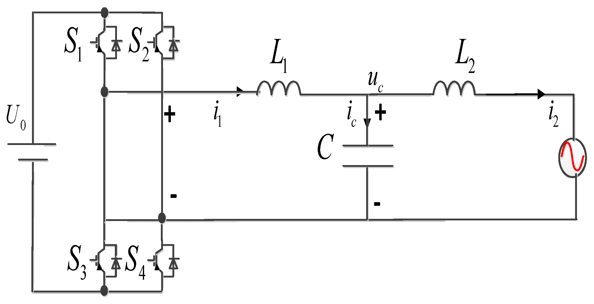
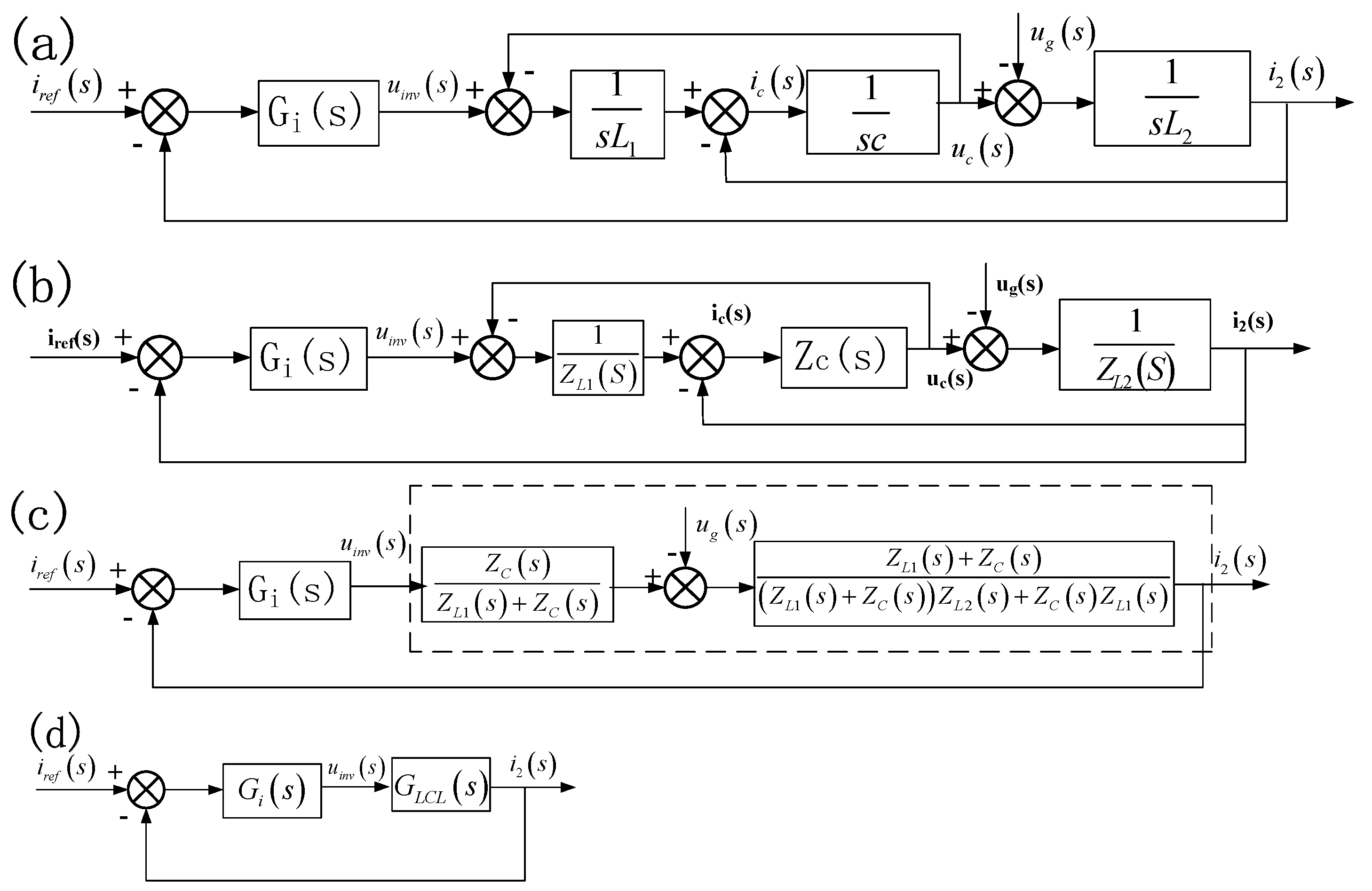
2. Control Strategy and Output Impedance of the LCL GCI

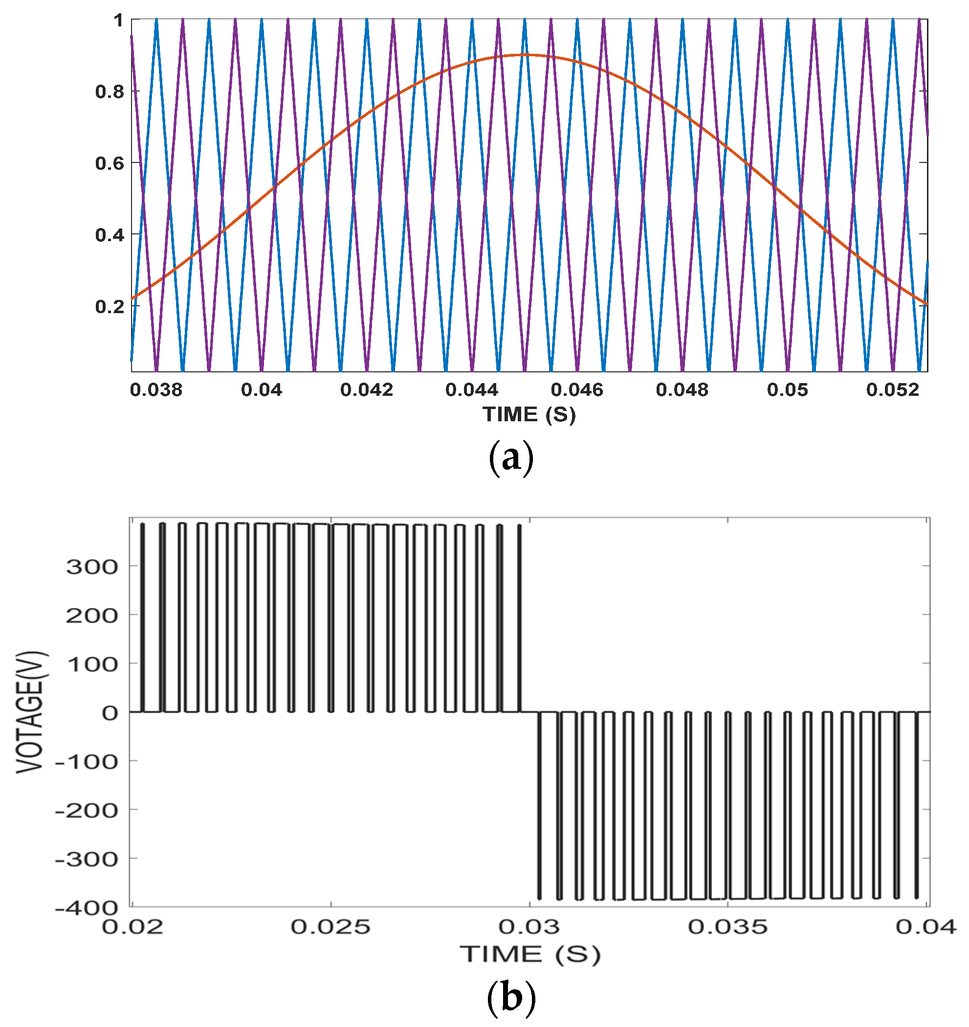
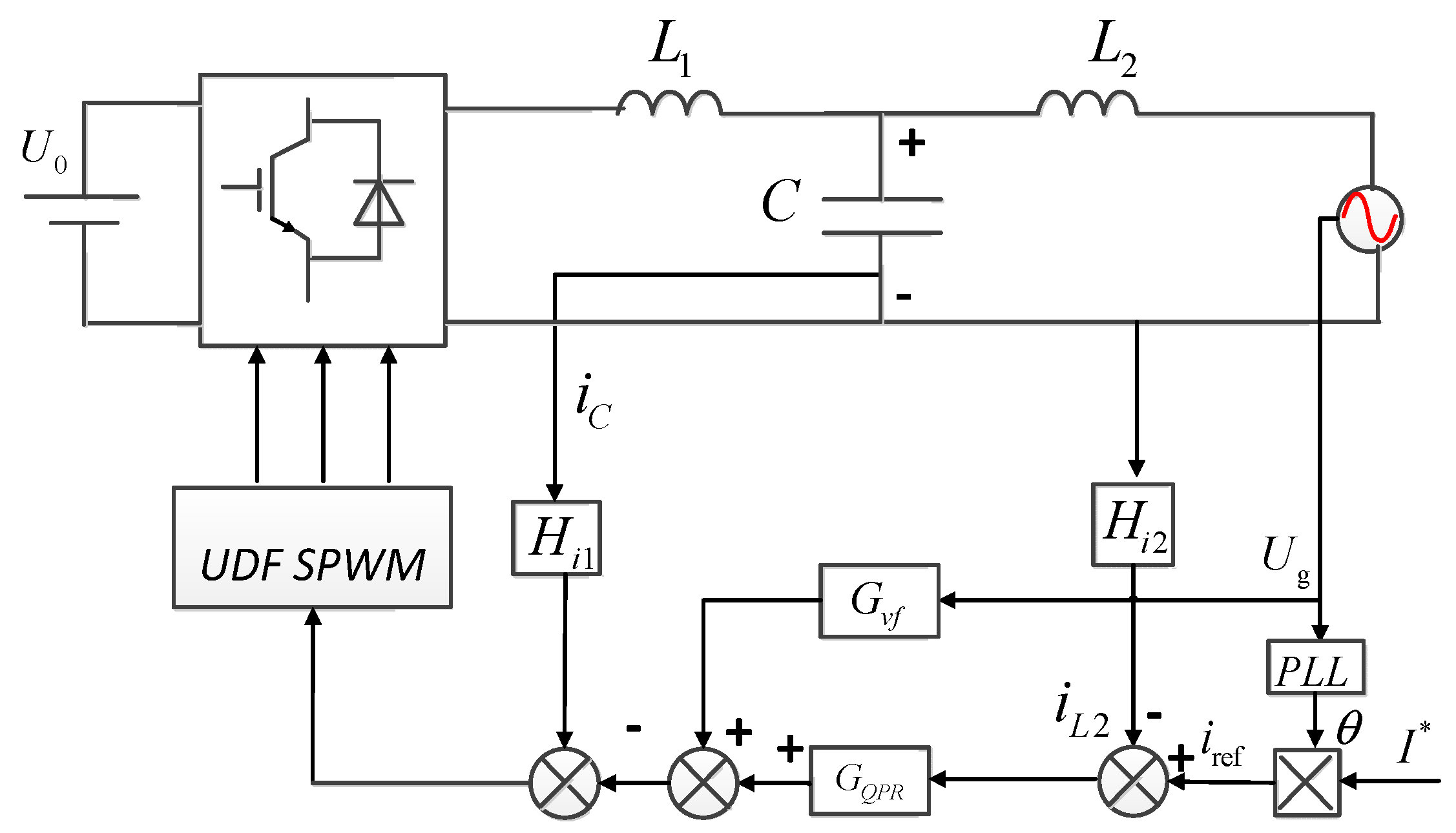
2.1. Unipolar Double-Frequency (UDF) SPWM

Sinusoidal pulse width modulation (SPWM) methods can be divided into bipolar, unipolar, and hysteresis comparison methods. As is widely known, bipolar SPWM modulation is the most common adjustment method. It involves comparing a sinusoidal signal with a given carrier wave, as shown in Figure 1a. This comparison then controls the high-frequency switching of the inverter switches between on and off for each pair of combinations, as illustrated in Figure 1b. However, its output voltage $U_{inv}$ is large, fluctuating from $U_{DC}$ to −$U_{DC}$; due to the distributed capacitance in the surroundings, the output current $I_{inv}$ exhibits significant fluctuations, making the inverter prone to damage. Additionally, its switching frequency is equal to the carrier frequency, resulting in relatively high switching losses [26].

UDF SPWM involves comparing the sinusoidal reference signal with two carrier waves that have phase differences of 0° and 180°, respectively, as shown in Figure 2a. The orange line is the sinusoidal signal, the purple line is the carrier, and the blue line is the carrier with a phase difference of 180°. Here, the four switches of the H-bridge inverter are denoted as g1, g2, g3, and g4. The relationship between the given sinusoidal signal and the carrier wave controls switches g1 and g2. Specifically, when the given sinusoidal signal is greater than the carrier wave, g1 is turned on and g2 is turned off. Simultaneously, the switches g3 and g4 are switched when the given sinusoidal signal and the carrier wave have a phase difference of 180° In this case, when the result is greater than a certain value, g4 is turned on, and g3 is turned off. The output voltage $u_{inv}$ is the voltage at the H-bridge output port, which is the difference in port potentials. Due to this difference, the frequency of the square wave voltage at output $U_{inv}$ becomes doubled, as depicted in Figure 2b.

It can be observed that the output voltage of UDF SPWM is the same as the unipolar modulation method. However, its input carrier frequency is half that of the unipolar frequency. Based on Equation (1), the filter inductor L is related to the output voltage square wave frequency $f_s$. The higher the frequency, the smaller the filter inductor required, reducing the cost and volume of the filter. The current $I_{max}$ is kept at a constant value to minimize the current ripple. At the same time, the output voltage $U_{inv}$ changes between $U_{DC}$and 0 during the positive half-cycle of the fundamental frequency and between 0 and −$U_{DC}$during the negative half-cycle, resulting in smaller fluctuations in the output current $I_{inv}$. Therefore, the unipolar multiplicative SPWM modulation is chosen [27].

$$L\ge \frac{U_{DC}}{4\Delta I_{MAX}{f}_s}$$

(1)

Phase-locked loop design. Using the Second-Order Generalized Integrator Phase-Locked Loop (SOGI PLL), the primary objective is to decompose a single sine signal into two orthogonal sine signals, enabling independent control of active and reactive power. Due to the fact that sine signals exhibit a second-order resonant section model in the s-domain, it is commonly referred to as a Second-Order Generalized Integrator (SOGI).

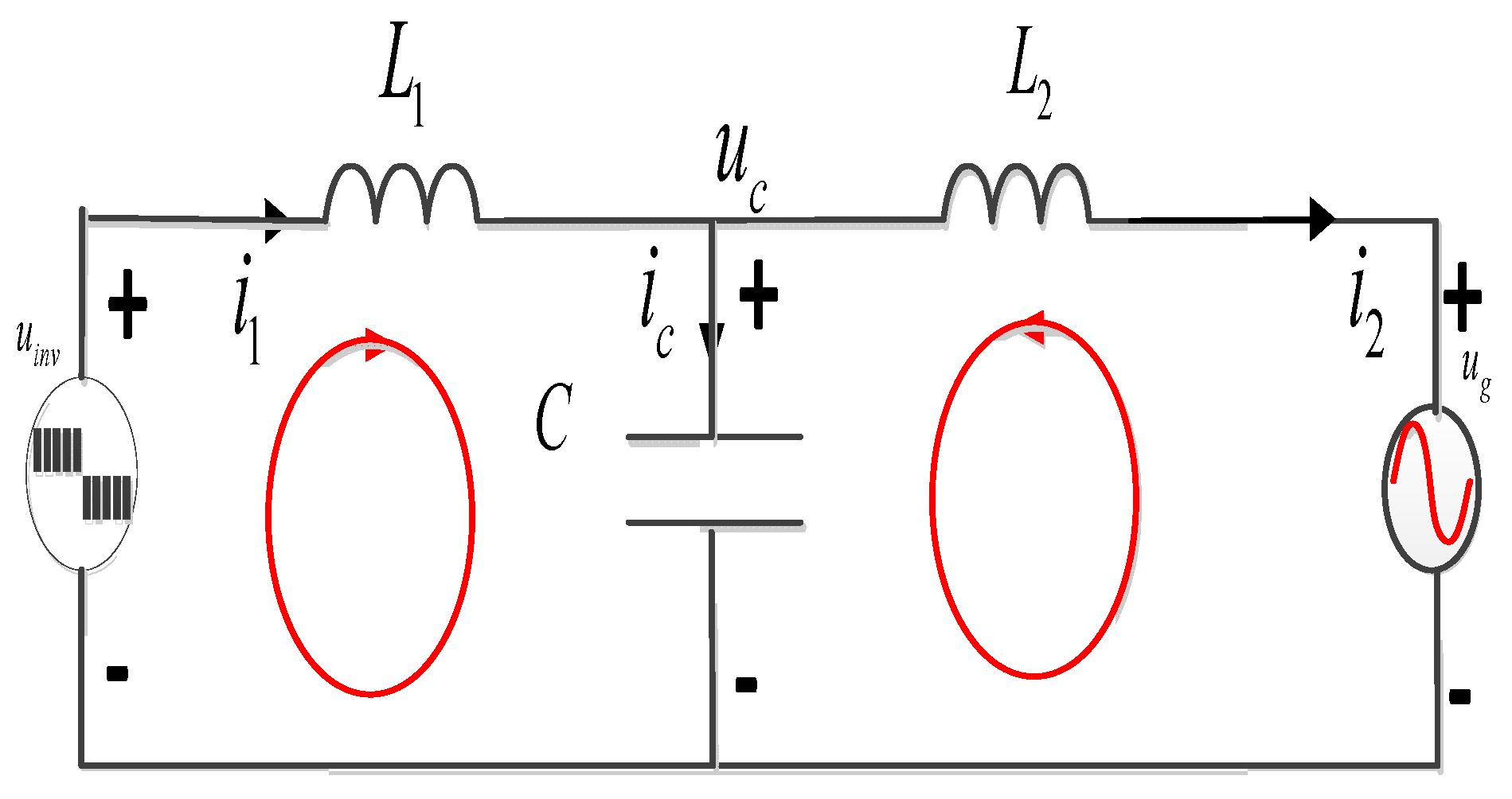
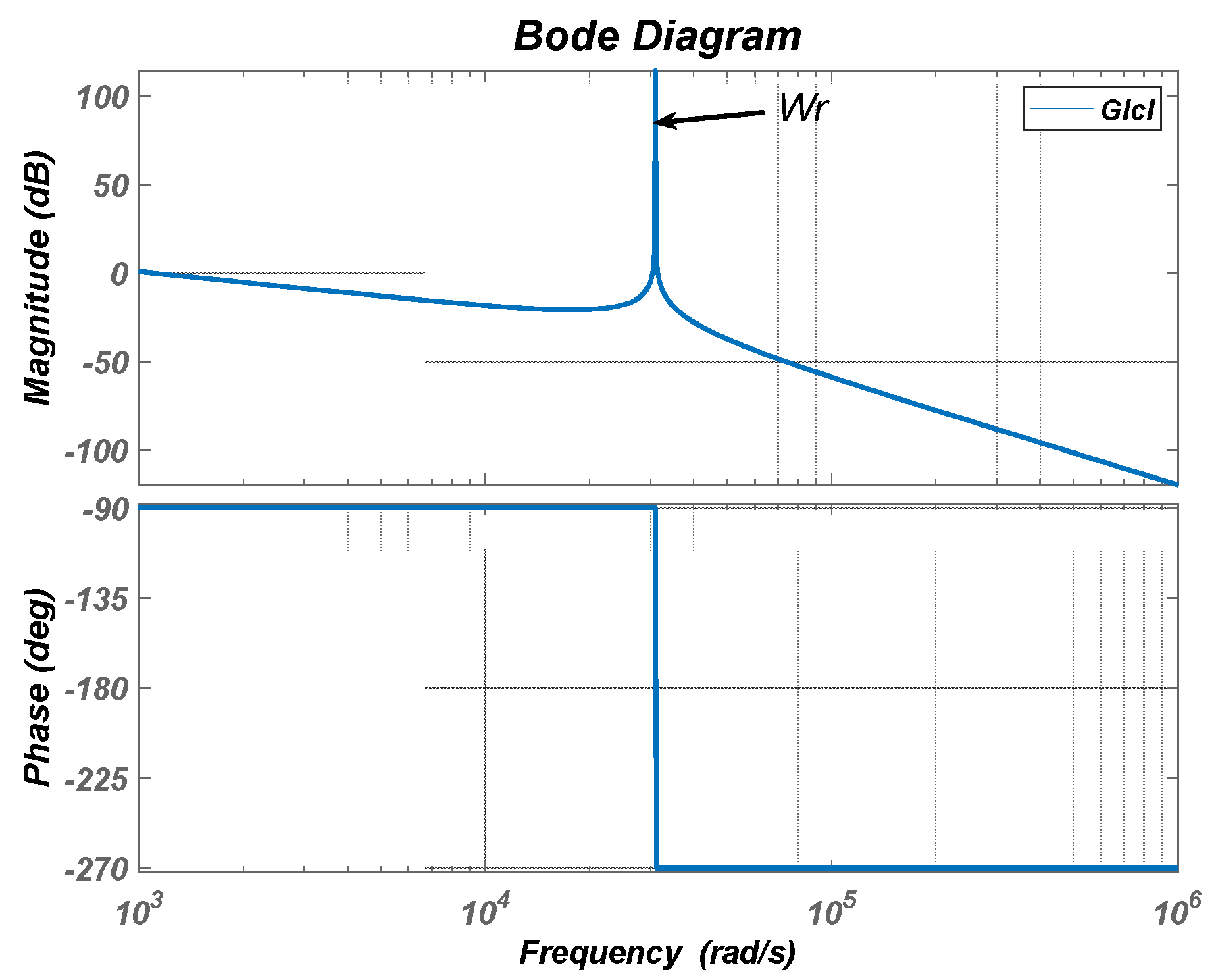
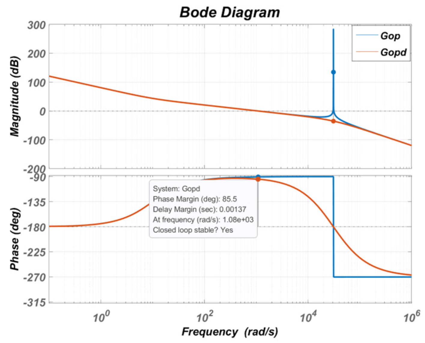
2.2. Stability Analysis of the LCL GCI

Due to the LC filter, when connected to the grid, the capacitor C is controlled by the grid, rendering it ineffective for filtering. In this scenario, the LC filter can only be considered as if L plays the role of filtering. When using only an L filter, a large inductance value is required to meet the grid requirements. Therefore, the LCL filter can reduce the inductance on the inverter side, simultaneously satisfying the grid requirements. A single LCL GCI, when connected to the grid, exhibits excellent filtering compared to an LC-type inverter, as shown in Figure 3. In this figure, $L_1$ represents the inverter-side inductance, $L_2$ is the grid-side inductance, and the filtering capacitor is denoted as C [28,29].

The LCL part of a single LCL inverter is equivalent to the block diagram shown in Figure 4, where $U_{inv}$ is the excitation source of the output of the inverter. In the S domain, KVL and KCL equations can be obtained.

$$U_{inv}\left(s\right)=L_{1}s{i}_1\left(s\right)+U_C\left(s\right)$$

(2)

$$U_C\left(s\right)=L_{2}s{i}_2\left(s\right)+U_g\left(s\right)$$

(3)

$$\begin{array}{l}{i}_1\left(s\right)=i_c\left(s\right)+i_2\left(s\right)=sC{U}_C\left(s\right)+i_2\left(s\right)\\ =sC\left(L_{2}s{i}_2\left(s\right)+U_g\left(s\right)\right)+i_2\left(s\right)\end{array}$$

(4)

By combining Equations (2)–(4), yields

$$U_{inv}\left(s\right)=L_{1}s\left[sC\left(L_{2}s{i}_2\left(s\right)+U_g\left(s\right)\right)+i_2\left(s\right)\right]+L_{2}s{i}_2\left(s\right)+U_g\left(s\right)$$

(5)

and by simplifying it, the relationship between $u_{inv}$ and $i_2$ can be obtained.

$$U_{inv}\left(s\right)=L_1{L}_{2}C{s}^3{i}_2\left(s\right)+\left(L_1+L_2\right)s{i}_2\left(s\right)+\left(L_{1}C{s}^2+1\right)U_g\left(s\right)$$

(6)

In order to facilitate analysis, the relationship between GCC $i_2$ and inverter input voltage $U_{inv}$ can be obtained without looking at the influence of GCV $u_g$ on $i_2$, as shown in Equation (7).

$$\begin{array}{l}\frac{i_2\left(s\right)}{U_{inv}\left(s\right)}=\frac{1}{L_1{L}_{2}C{s}^3+\left(L_1+L_2\right)s}=\frac{1}{\left(L_1+L_2\right)s}\frac{\frac{\left(L_1+L_2\right)}{L_1{L}_{2}C}}{\left(s^2+\frac{\left(L_1+L_2\right)}{L_1{L}_{2}C}\right)}\\ =\frac{1}{\left(L_1+L_2\right)s}\frac{{\omega }_r}{\left(s^2+{\omega }_r\right)}\end{array}$$

(7)

$${\omega }_r=\sqrt{\frac{\left(L_1+L_2\right)}{L_1{L}_{2}C}}$$

(8)

Setting ${\omega }_r$ to the resonant angular frequency in Equation (8), when the frequency is ${\omega }_r$, the gain of the transfer function is infinite; that is, the current $i_2$ will diverge. By setting the parameters ${\omega }_r$to the usual requirements of ${f_o<\omega }_r<$0.5 $f_s$, the filter becomes more efficient and the harmonics of the GCC $i_2$ are lower.

Figure 5 is a Bode diagram of the $G_{LCL}$ open-loop transfer function. The parameter values are provided in

Table 1. Parameters.

Pa Parameters and Symbols	Values	Parameters and Symbols	Values
Input voltage $U_0$	400 V	Grid-side inductor $L_2$	0.00012 H
Grid voltage $U_g$	220 V	Carrier amplitude $V_T$	1 V
Fundamental frequency $f_0$	50 Hz	Carrier frequency $f_T$	10 kHz
Switching frequency $f_s$	20 kHz	Proportional coefficient of $G_{QPR}\left(Z\right)$ and $G_{PI}\left(Z\right)$Kp	10
Inverter-side inductor $L_1$	0.000 H	Integral coefficient of $G_{QPR}\left(Z\right)$KR	1000
Filter capacitor C	10 $\mu f$	Integral coefficient of $G_{PI}\left(Z\right)$ KI	1000
Grid current sensor gain Hi1	1	Sampling period $T_S$	50$\mu s$
Feedback coefficient of capacitor-current Hi2	32	Cutoff frequency ${\omega }_c$	5

.

From the Bode plot, it can be observed that the LCL filter exhibits good filtering performance. As the frequency increases, its gain continuously decreases, indicating improved filtering effectiveness. However, there is a peak in the graph, occurring at the resonant angular frequency${ \omega }_r$. At this frequency, harmonics are amplified, and, simultaneously, there is a phase transition from −90° to −270°. The phase margin is less than 180°, making it prone to instability in closed-loop systems.

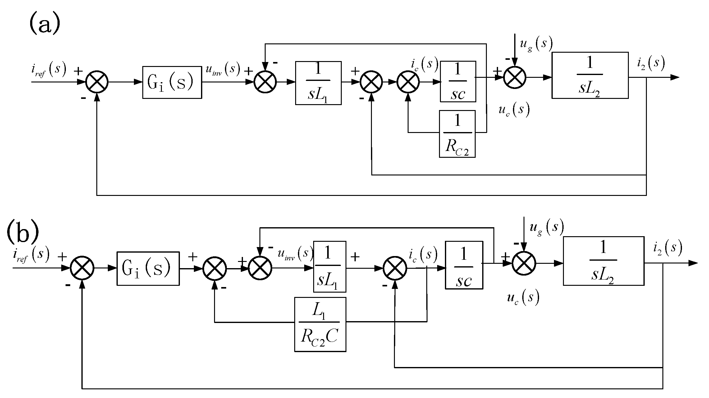
2.3. Active-Damped LCL GCI

In order to suppress the impact of resonance on the grid inverter, damping needs to be introduced. This involves introducing the square term of s into the denominator of Equation (7), shown in Equation (9).

$$G_{LCL-d}\left(s\right)=\frac{i_2\left(s\right)}{U_{inv}\left(s\right)}==\frac{1}{\left(L_1+L_2\right)s}\frac{{\omega }_r}{\left(s^2+2\delta {\omega }_{r}s+{\omega }_r\right)}$$

(9)

Following the introduction of closed-loop control, the control block diagram is depicted in Figure 6a. The grid current $i_2$ is compared with the reference current $i_{ref}$. Through the controller, for analytical simplicity, a basic proportional-integral controller $G_i$ is employed. Subsequently, the output goes through UDF to control the inverter-side voltage $U_{inv}$. Setting $Z_1\left(s\right)=s{L}_1$, $Z_C\left(s\right)=1/sC$, and $Z_2\left(s\right)=s{L}_2$, then the control block diagram can be equivalent to Figure 6b for simplification, and, finally, the control block diagram in Figure 6c can be obtained.

Disregarding the disturbance of $U_g$ on the system, the dashed portion in Figure 6c is replaced by $G_{LCL}$, resulting in the final control block diagram in Figure 6d. For stability analysis of the control system, the open-loop transfer function $G_{OP}$ is utilized, expressed as Equation (10). Its Bode plot is illustrated in Figure 7. Stability analysis focuses on the phase response when crossing 0 dB. The phase must be above −180° for a positive phase margin, ensuring system stability; otherwise, instability may occur.

Replacing $G_{LCL}$ with the transfer function $G_{LCL-d}$ after introducing damping and properly designing $\delta$ such that its open-loop transfer function is $G_{OPd}$, the resulting Bode plot is shown in Figure 7. It can be observed that, by appropriately designing the value of $\delta$, it is possible to ensure that the amplitude at the resonance frequency point ${\omega }_r$ does not pass through the 0 dB point, thereby having no effect on the stability of the system [30].

$$G_{OP}\left(s\right)=G_i\left(s\right)G_{LCL}\left(s\right)$$

(10)

2.4. Analysis of the Active-Damped LCL GCI

In the introduction of passive damping analysis, the ultimate effect is achieved by adding a resistor across the capacitor terminals. This is illustrated in the control block diagram in Figure 8a, where $1/R_{C2}$ represents the control loop and represents the parallel resistor in the capacitor. By rational simplification through control principles, active damping control is obtained without the need for a parallel resistor. The input node of the control loop $1/R_{C2}$ is moved to node $G_i$, and the output node is also moved forward to node $1/s{L}_1$, resulting in the control block diagram in Figure 8b. Through this simplification, the loop can be controlled, and the impact of differentiation is eliminated. This is crucial because differentiation amplifies noise, and discrete differentiation introduces errors, weakening the effectiveness of active damping. However, it is necessary to introduce the capacitor current $i_c$ into the main circuit, along with the proportional coefficient $H_1=L_1/R_{C2}C$ in the control loop. This is referred to as the active damping grid current and capacitor current dual feedback control strategy, and the resulting diagram is shown in Figure 9, where Hi1 is the capacitor current feedback coefficient and Hi2 is the grid current feedback system. In the active damping system, Zc is the sum of the capacitor and the parallel resistance [31,32], so

$$Z_C=\frac{R_{C2}}{S{R}_{C2}+1}$$

(11)

3. Proportional-Resonance Controller Based on a Voltage Weight Feedforward Scheme for LCL GCV

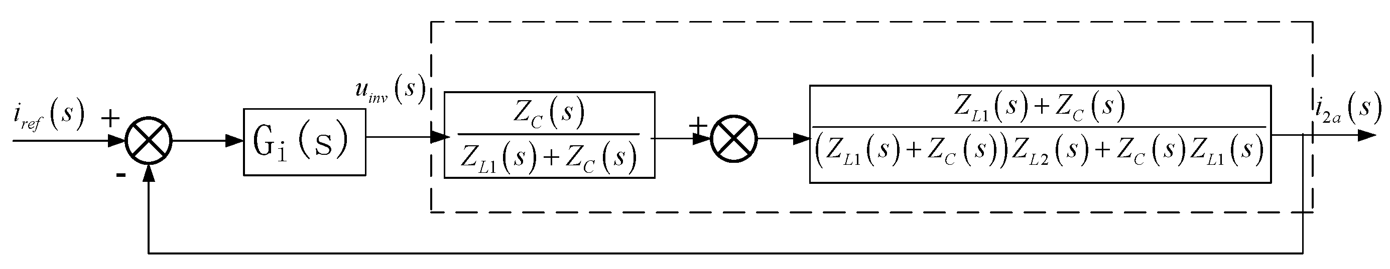
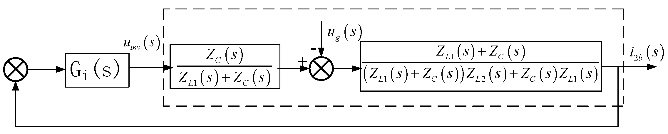
3.1. Analysis of the Influence of Power Grid Voltage on LCL Inverter

Considering the power grid voltage stability analysis, as shown in Figure 10, setting $G_1\left(s\right)=Z_C\left(s\right)/\left(Z_{L1}\left(s\right)+Z_C\left(s\right)\right)$, $G_2$ can be expressed as per Equation (12).

$$G_2\left(s\right)=\frac{Z_{L1}\left(s\right)+Z_C\left(s\right)}{\left(Z_{L1}\left(s\right)+Z_{L2}\left(s\right)\right)Z_{L2}\left(s\right)+Z_C\left(s\right)Z_{L1}\left(s\right)}$$

(12)

The superposition theorem is used to analyze it, respectively. Firstly, the influence of GCV $U_g$ is not considered,

$$G_{ii}\left(s\right)=\frac{i_{2a}\left(s\right)}{i_{ref}\left(s\right)}=\frac{G_i\left(S\right)G_1\left(S\right)G_2\left(S\right)}{1+G_{op}\left(S\right)}$$

(13)

Similarly, the input current $i_{ref}$ is not considered; only the influence of GCV is considered, as shown in Figure 11.

$$G_{iv}\left(s\right)=\frac{i_{2a}\left(s\right)}{-U_g\left(s\right)}=\frac{G_2\left(S\right)}{1+G_{op}\left(S\right)}$$

(14)

$i_{2a}$ is the output current when there is only a reference current $i_{ref}$ input, $i_{2b}$ is the output current when there is only a $U_g$ input, and $i_2$ is the output grid current.

$$i_2=i_{2a}+i_{2b}=i_{ref}\left(s\right)G_{ii}\left(s\right)-U_g\left(s\right)G_{iv}\left(s\right)$$

(15)

Using this equation, it can be observed that $G_{iv}$ reflects the tracking performance of the given current, while $G_{ii}$ responds to the disturbance effects of the grid voltage. Here, tracking performance mainly refers to the function of $i_{ref}$ in Equation (13). From Equations (14) and (15), it can be seen that if the magnitude of the outer loop gain $G_i$ is sufficiently large, the variation caused by $U_g$ can be greatly reduced. However, adopting the most basic PI controller may result in lower control accuracy for tracking and make the changes induced by $U_g$ more significant [33,34].

3.2. Proportional Resonance (PR) Controller

The PR controller has infinite gain at the fundamental frequency and very small gain at non-fundamental frequencies. Therefore, the system can achieve zero steady-state error at the fundamental frequency. At the same time, based on the analysis of the grid voltage $U_g$ mentioned above, when the gain is sufficiently large, it significantly reduces the impact of the changes induced by $U_g$.

The transfer function of the PR controller is

$$G_{PR}\left(s\right)=k_p+\frac{2k_{r}s}{s^2+{w_0}^2}$$

(16)

In Equation (16), K_p is the proportional coefficient, and K_r is the integral coefficient. ${\omega }_0=2\pi f_0$ where f is the frequency of the fundamental wave. The inverter output current is related to the reference current and grid voltage. For PI control, the gain of the controller at the fundamental frequency ${\omega }_0$ is finite, while for PR control, the gain of the controller at the fundamental frequency ${\omega }_0$ tends to infinity. Therefore, PR control can achieve zero steady-state error and has the ability to resist grid voltage disturbances. The Bode plot of the open-loop transfer function $G_{PR}$ is shown in Figure 12a, with parameters set as in Table 1. It can be observed that the gain is extremely high at the specified fundamental frequency.

In practical systems, due to issues with the implementation of PR controllers, where the gain becomes infinite at 50 Hz, fluctuations may occur since the grid frequency may not strictly equal 50 Hz. When the frequency deviates slightly from 50 Hz, the gain significantly attenuates. To enhance control robustness, a commonly employed approach is to use a QPR, which is easier to implement. Its open-loop transfer function is given by Equation (17), where ${\omega }_c$ is the cutoff frequency, as depicted in the Bode plot in Figure 12b.

$$G_{QPR}\left(s\right)=k_p+\frac{2k_{r}s}{s^2+2{\omega }_{C}s+{w_0}^2}$$

(17)

From the Bode plot, it can be observed that as K_p increases, the gains in other low-frequency and high-frequency ranges become larger. Similarly, with an increase in K_r, the gain at the resonance point becomes larger, but the gains in the surrounding frequency bands also increase accordingly. As $\omega$ increases, the gains in the surrounding frequency bands also increase correspondingly.

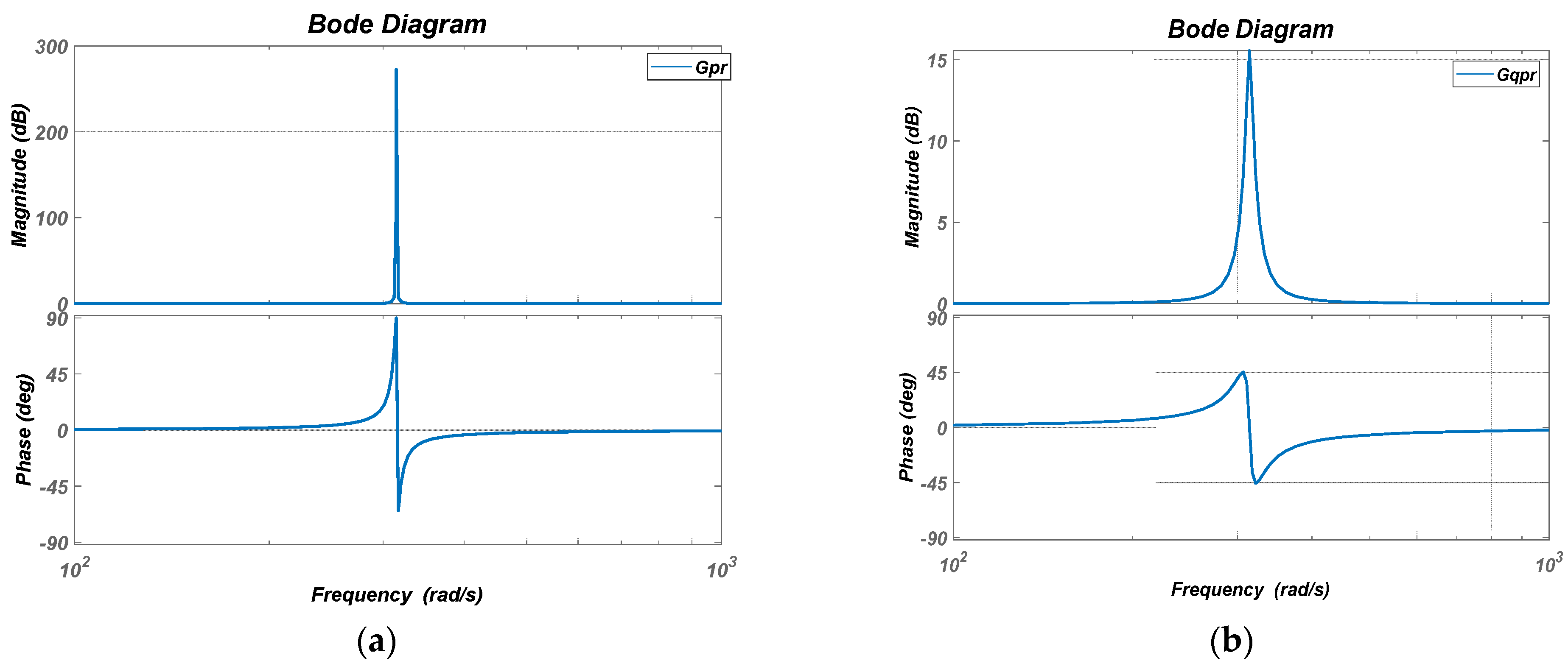
3.3. Grid-Voltage-Weighted Feedforward Scheme Based on the QPR

According to Equation (15), it can be understood that the impact of the grid voltage on the system is denoted by $U_g·G_{iv}$. Injecting this compensating term into the control system will eliminate the influence of $U_g$ on the inverter, as expressed in Equation (18). In the representation of the control block diagram, introducing the forward transfer function $G_2$ between $U_g$ and $i_2$ at the front end of node $i_2$ is illustrated in Figure 13a. Through simplification, by moving the input node of this term to the $G_{QPR}$ node, the feedforward function ${1/G}_2$ will eliminate the impact of $U_g$ on the injected current $i_2$, as shown in Figure 13b. Expanding and restoring the control block diagram, moving the feedforward function${ 1/G}_2\left(s\right)$ to the$G_{QPR}$ node, the resulting feedforward function is ${ 1/G}_1\left(s\right)$, as shown in Figure 13c.

$$i_2=i_{ref}\left(s\right)G_{ii}\left(s\right)-U_g\left(s\right)G_{iv}\left(s\right)+U_g\left(s\right)G_{iv}\left(s\right)$$

(18)

Setting ${ G_{vf}=1/G}_1\left(s\right)$, then expanding and simplifying it, yields

$$G_{vf}\left(s\right)=s^2{L}_{1}C+\frac{L_1}{R_{C2}}S+1$$

(19)

From Equation (19), a function with second-order derivative components and first-order derivative components can be obtained. Compensating for these three terms will eliminate the influence of grid voltage feedback on the system. The influence of grid voltage is mainly manifested in the effects of harmonics and voltage variations.

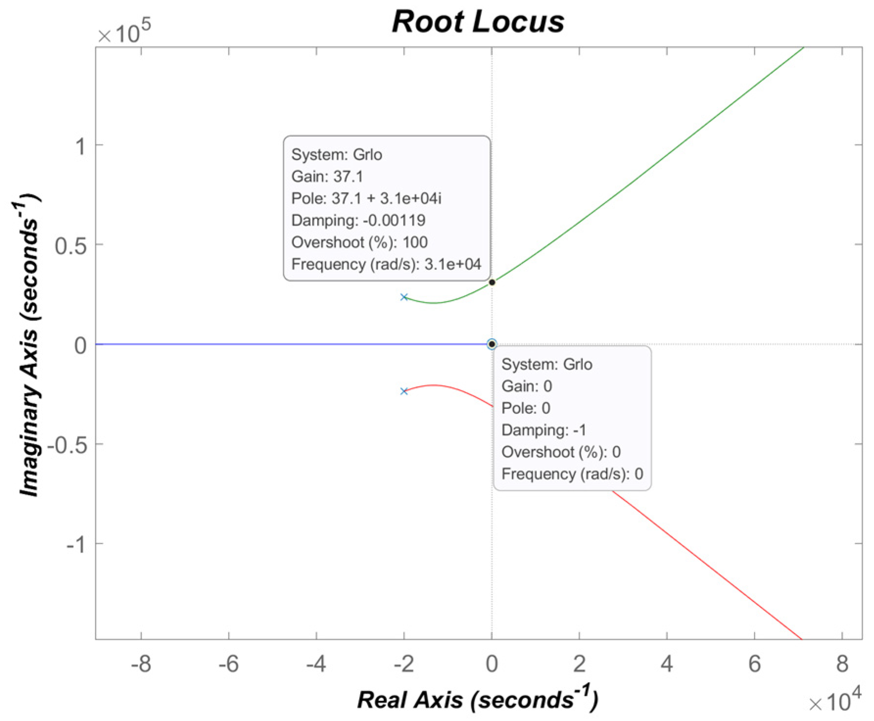
3.4. Stability Analysis of Voltage Full Feedforward in the QPR Controller

The use of the QPR controller voltage full feedforward scheme can minimize the impact of grid voltage on the control strategy; stability analysis is performed.

First, the parameter settings of the QPR controller need to be determined. The cutoff frequency ${\omega }_c$, in the quasi-resonant controller, not only affects the gain of the controller but also influences the controller’s bandwidth. With an increase in ${\omega }_c$, the gain of the controller increases, and the bandwidth of the quasi-resonant controller is given by ${\omega }_c/2\pi$ Hz. Typically, considering the allowable fluctuation range of the grid frequency as ±0.8 Hz, this implies ${\omega }_c/2\pi$ = 1.6 Hz, i.e., ${\omega }_c$ = 5. The determination of K_p and K_r is achieved through root locus analysis. Initially, set the value of K_R as 1 and use the root locus plot to determine the range of K_R values. In the root locus plot, the root locus values on the left half-plane of the real axis indicate system stability, whereas those on the right half-plane are unstable. Moreover, roots farther away from the imaginary axis are more stable. As shown in Figure 14, it is evident that the minimum value for K_p is 0, and the maximum value is 37. Both 0 and 37 are critical values lying on the imaginary axis. To ensure stability, a middle value of 12 is chosen for K_p.

Next, analyze and determine the value of K_R through the Bode plot in Figure 15. To ensure a certain stability margin, it is typically required that the phase margin of the open-loop transfer function be set to be 30 or above. Simultaneously, to ensure a certain response filtering effect, the closed-loop transfer function is usually chosen to be between 1/10 and 1/2 of the fluctuation frequency of the $U_{ab}$ square wave. The fluctuation frequency of the $U_{ab}$ square wave in the system is 20 kHz, and the most suitable range is considered to be between 4000 and 6000.

In the Bode plot, $G_{op1}$ represents the open-loop transfer function. Bode plot with K_r set to 10, $G_{op2}$ represents the open-loop Bode plot with K_r set to 1000, and $G_{op3}$ represents the open-loop Bode plot with K_r set to 10,000. It can be observed that using the QPR controller results in a peak in the amplitude gain at the fundamental frequency, where the gain is amplified. Additionally, as K_p increases, the gain at the fundamental frequency also increases. However, this also amplifies the gain near the fundamental frequency, making it prone to generating harmonics at nearby frequencies. Meanwhile, the phase margin exceeds 30°. $G_{op2}$ has a phase margin of 54.8, and $G_{op3}$ has a phase margin of 44.3. The larger the phase margin, the more stable the system. Considering these factors, a K_r value of 1000 is chosen.

$G_{CL1}$ represents the Bode plot of the system’s closed-loop transfer function. It is observed that the bandwidth frequency, i.e., the frequency at which the gain is −3 dB, is 4300 Hz, which falls within the design requirement range of 4000–6000 Hz.

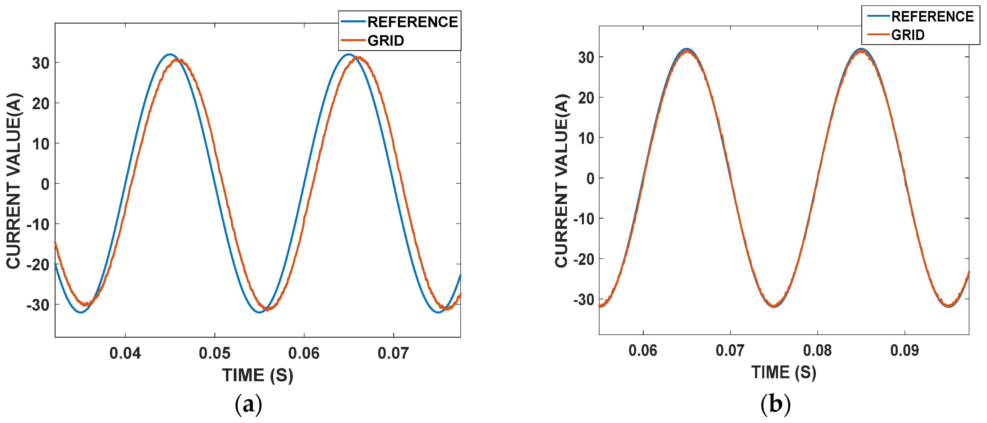
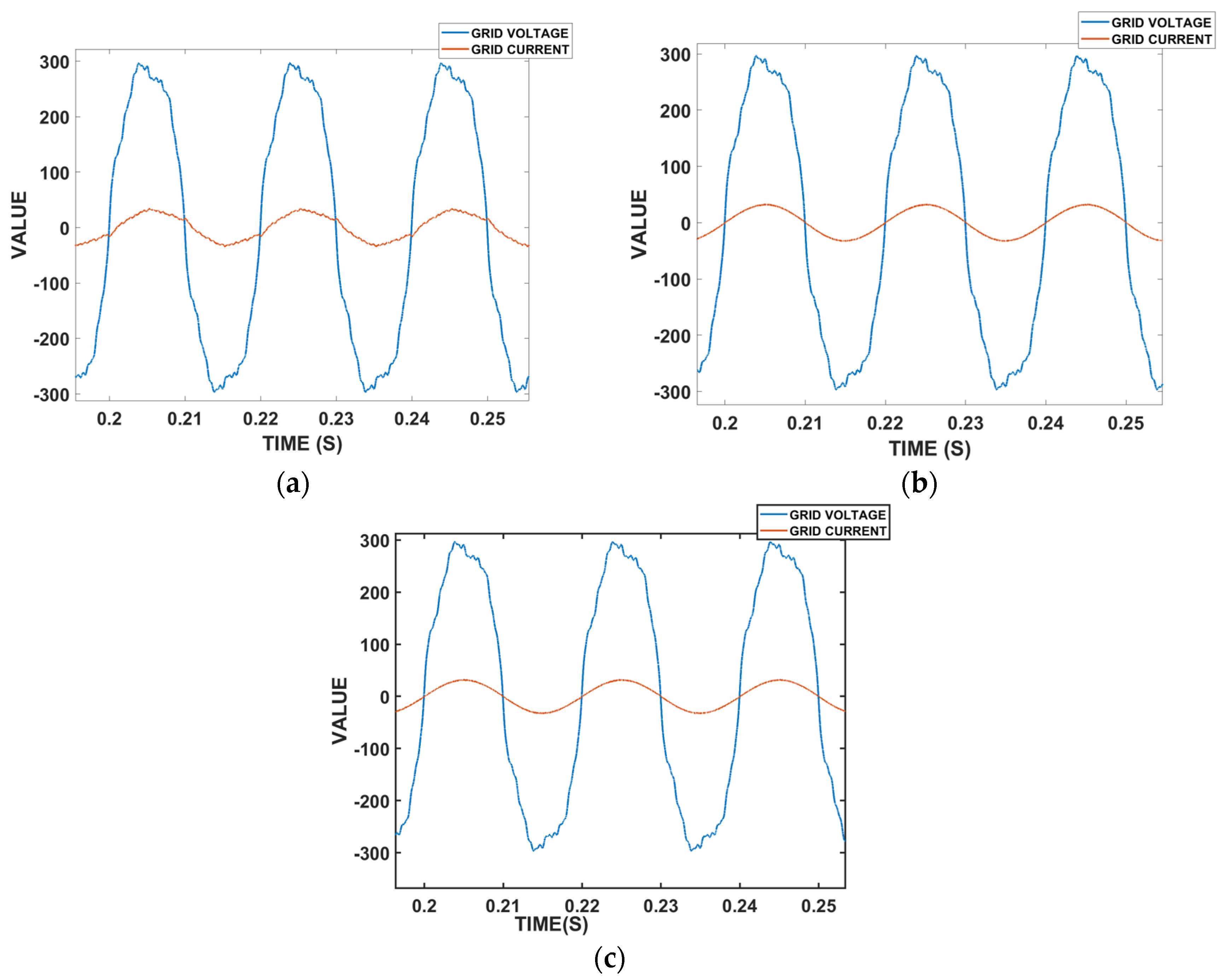
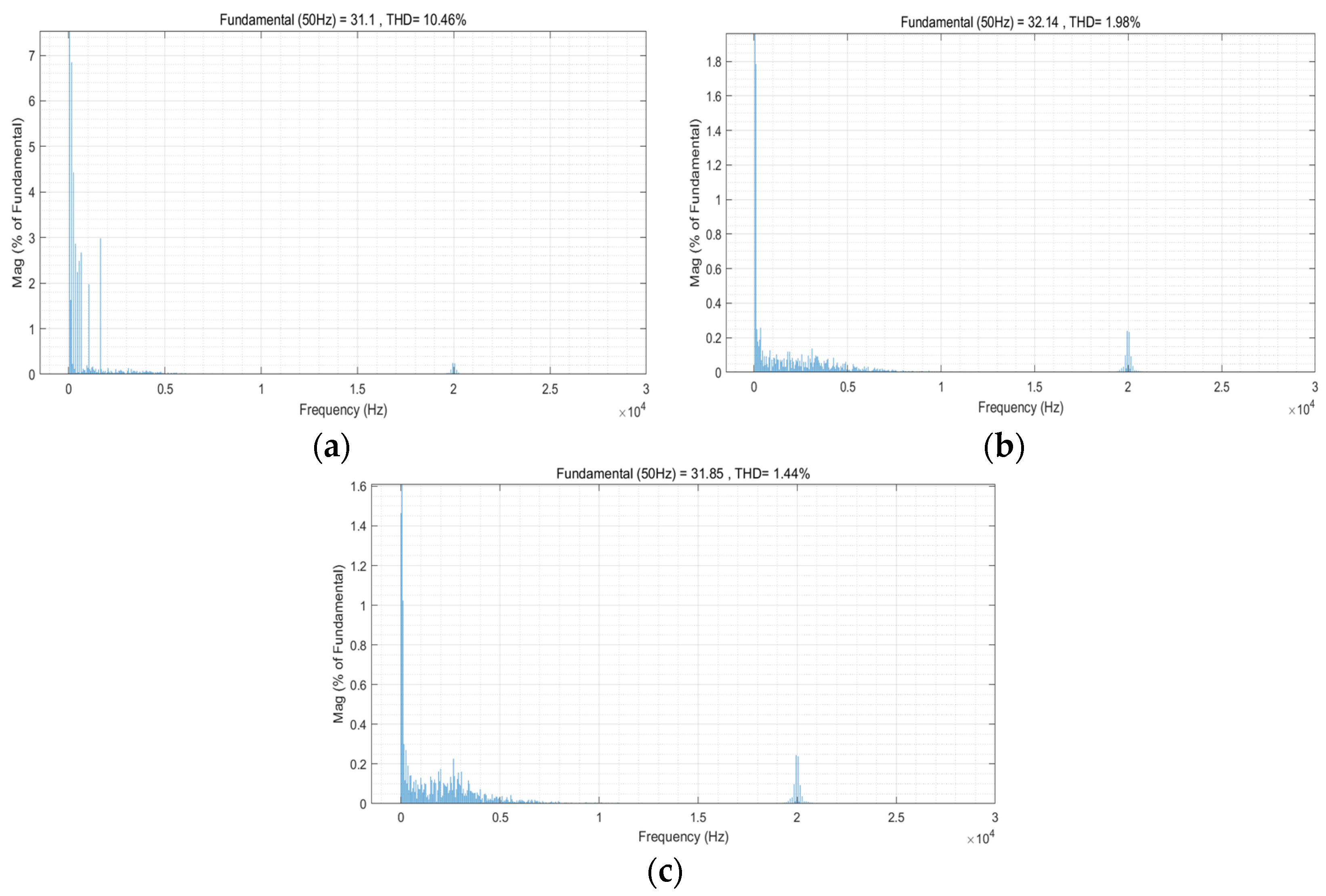
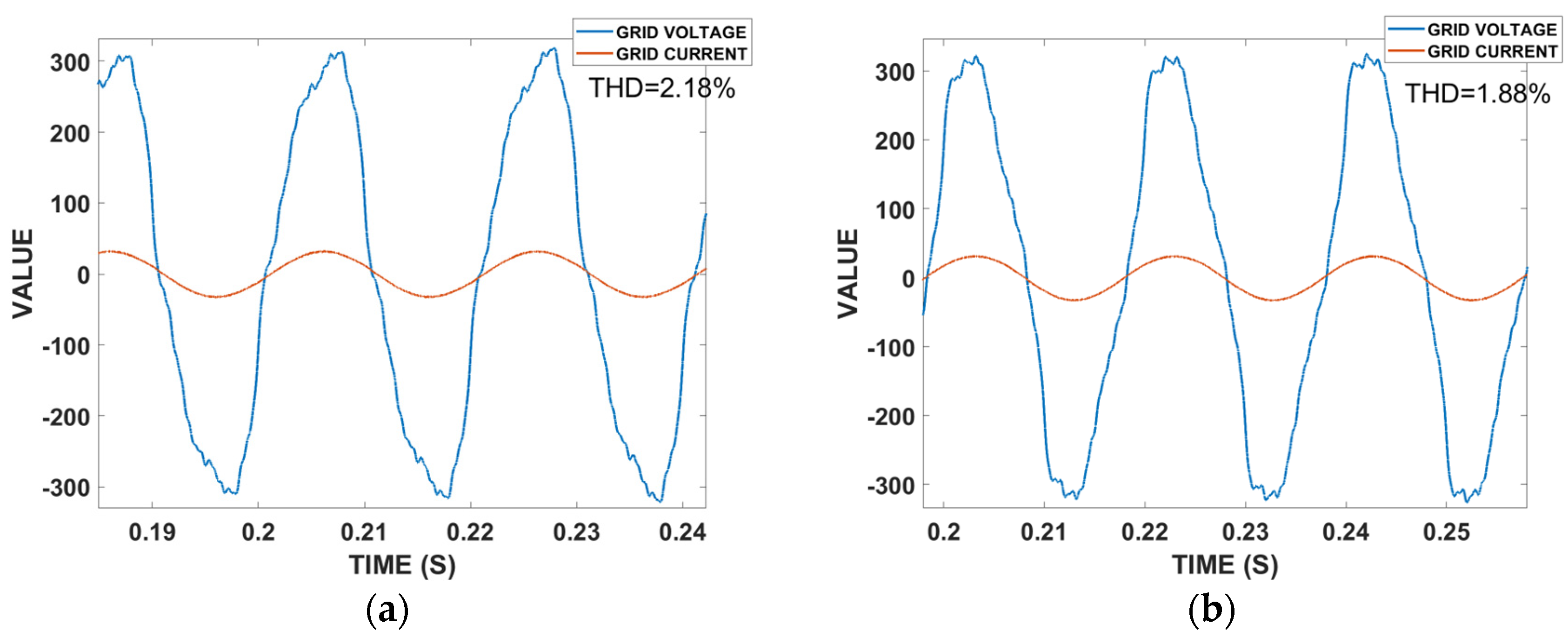
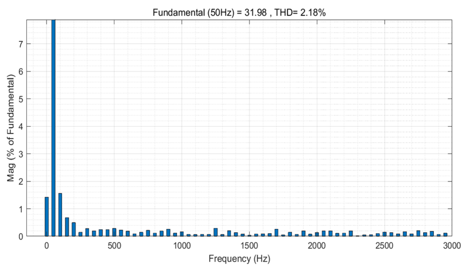
4. Experimental Results

To validate the proposed grid-voltage-weighted feedforward scheme based on the QPR controller, a discrete simulation is conducted. The control system needs to be discretized for the simulation. Two controllers, namely the PI controller and the QPR controller, are selected for comparison in the experiment. Both controllers need to be discretized, transforming them into models in the Z-domain. The bilinear transformation method is employed; the equation is 20, where Ts denotes the sampling period.

$$G\left(z\right)=G\left(s\right){|}_{s=\frac{2}{T_S}\frac{Z-1}{Z+1}}$$

(20)

The expression for s in the continuous transfer function is given by

$$s=\frac{2}{T_S}\frac{Z-1}{Z+1}$$

(21)

First, discretize the $G_{PI}\left(s\right)$ controller

$$G_{PI}\left(s\right)=K_P+K_I/s$$

(22)

Can be obtained

$$G_{PI}\left(Z\right)=k_p+K_i\cdot T_{\mathrm{s}}\left(Z+1\right)/2\left(Z-1\right)$$

(23)

In discretizing the QPR controller, Equation (21) is brought into Equation (17) to obtain Equation (24).

$$G_{QPR}\left(Z\right)=k_p+\frac{2k_r\left(\frac{2}{T_S}\frac{Z-1}{Z+1}\right)}{{\left(\frac{2}{T_S}\frac{Z-1}{Z+1}\right)}^2+2{\omega }_C\left(\frac{2}{T_S}\frac{Z-1}{Z+1}\right)+{w_0}^2}$$

(24)

Simplifying it gives

$$G_{QPR}\left(z\right)=k_p+\frac{4k_r{T}_S{\omega }_C{z}^2-4k_r{T}_S{\omega }_C}{\left({T_s}^2{{\omega }_0}^2+4T_S{\omega }_C+4\right)z^2+\left(2{T_s}^2{{\omega }_0}^2-8\right)z+{T_s}^2{{\omega }_0}^2-4T_S{\omega }_C+4}$$

(25)

All the sampled signals in the system go through the sample-and-hold and calculation link, which are in perfect agreement with the results of the physical experiments.

The parameters in the system are listed in Table 1. To evaluate the proposed solution, simulate grid voltage harmonics, including background harmonics of the 3rd, 5th, 7th, 13th, 21st, and 33rd orders. The ratio and phase of each harmonic correspond to the fundamental voltage, as indicated in

Table 2. The amplitude ratio and relative phase of each harmonic correspond to the fundamental voltage.

Harmonic orders	3	5	7	13	21	33
Amplitude ratio (%)	33	21	13	7	5	3
Relative phase (°)	1	1	3	3	5	10

.

Figure 16a shows the comparison between grid current and the reference grid current obtained using a PI controller under normal grid voltage conditions (without simulated harmonics). It can be observed that the maximum value of the reference current is 32 A, while the grid current value is 31.4 A. At the same time, there is a significant phase difference between the grid current and the reference current, indicating poor tracking performance with a certain degree of error.

Figure 16b illustrates the grid current obtained with the QPR controller based on grid-voltage-weighted feedforward under normal grid voltage conditions. It can be seen that the grid current perfectly aligns and overlaps with the reference current, reflecting excellent tracking performance with minimal error.

Figure 17a: Comparison of grid current and grid voltage with a PI controller under grid voltage harmonics. Figure 17b: Comparison of the PI controller-based grid voltage feedback. Figure 17c: Comparison of QPR controller-based grid voltage feedback. Figure 18a: THD of the PI controller under grid voltage harmonics. Figure 18b: THD of PI controller-based grid voltage feedback. Figure 18c: THD of QPR controller-based grid voltage feedback.

Under grid voltage harmonics conditions, the ripple in the grid current generated by the PI controller is significant, and the harmonics are very large, resulting in a THD of 10.46%, which exceeds the specified standard and is not acceptable. Using the PI grid voltage feedback control system allows for normal operation with a THD of 1.98%. Meanwhile, with the QPR grid voltage feedback, the ripple is very small and is not affected by changes in the grid voltage, resulting in a THD of only 1.44%, demonstrating strong robustness.

While injecting simulated background harmonics according to the corresponding values in Table 2, the fundamental frequency of the grid voltage was altered to 49.5 and 50.5, respectively. Experiments were conducted using a QPR controller based on grid voltage feedback. The analysis of the output grid current quality yielded THD values of 2.18 and 1.88, as shown in Figure 19. Although the values have increased slightly, they remain within the normal stable range.

Simultaneously, a further analysis was performed on the THD with a fundamental frequency of 49.5, as shown in Figure 20. It can be observed that, after injecting 3rd, 5th, 7th, 13th, 21st, and 33rd harmonics, the output current harmonics were effectively suppressed compared to the injected harmonics. Only some harmonics were generated near the fundamental frequency, which is attributed to the impact of the fundamental frequency change on the system. However, due to the characteristics of the QPR controller, the system’s stability and tracking performance remained satisfactory. A single harmonic does not exceed the specified limit. Adjustments to QPR parameters can be made based on practical design needs. By changing ${\omega }_C$, the width of the frequency response can be adjusted to ensure system stability when the fundamental frequency changes within a certain range. However, it can also amplify range noise.

The above comparison further confirms that the tracking performance and robustness of this design scheme are both excellent.

5. Conclusions

This paper presents a QPR-based grid-voltage-weighted feedforward scheme for GCI with LCL filters. Utilizing the UDF SPWM method, the system performance has been analyzed under grid voltage disturbances. The study involves the use of a voltage feedforward weighted strategy and proportional-resonant controller with a thorough analysis of the rational design of various parameters. Experimental results indicate that the inverter performs well under normal grid conditions, weak grid conditions, and grid frequency fluctuations, effectively suppressing the impact of grid voltage disturbances on the system. The robustness of this inverter has been demonstrated, making it suitable for various complex grid voltage disturbance environments.

References

1. Blaabjerg, F.; Teodorescu, R.; Liserre, M.; Timbus, A.V. Overview of Control and Grid Synchronization for Distributed Power Generation Systems. IEEE Trans. Ind. Electron. 2006, 53, 1398–1409. [Google Scholar] [CrossRef]
2. Castilla, M.; Miret, J.; Matas, J.; Vicuna, L.G.; Guerrero, J.M. Control Design Guidelines for Single-Phase Grid-Connected Photovoltaic Inverters with Damped Resonant Harmonic Compensators. IEEE Trans. Ind. Electron. 2009, 56, 4492–4501. [Google Scholar] [CrossRef]
3. Liserre, M.; Teodorescu, R.; Blaabjerg, F. Stability of photovoltaic and wind turbine grid-connected inverters for a large set of grid impedance values. IEEE Trans. Power Electron. 2006, 21, 263–272. [Google Scholar] [CrossRef]
4. Liserre, M.; Teodorescu, R.; Blaabjerg, F. Multiple harmonics control for three-phase grid converter systems with the use of PI-RES current controller in a rotating frame. IEEE Trans. Power Electron. 2006, 21, 836–841. [Google Scholar] [CrossRef]
5. Twining, E.; Holmes, D.G. Grid current regulation of a three-phase voltage source inverter with an LCL input filter. In Proceedings of the 2002 IEEE 33rd Annual IEEE Power Electronics Specialists Conference, Proceedings (Cat. No.02CH37289), Cairns, QLD, Australia, 23–27 June 2002; pp. 1189–1194. [Google Scholar]
6. Walker, H.A.; Thye, S.R.; Simpson, B.; Lovaglia, M.J.; Willer, D.; Markovsky, B. Network exchange theory: Recent developments and new directions. Soc. Psychol. Q. 2000, 63, 324–337. [Google Scholar] [CrossRef]
7. Charin, C.; Ishak, D.; Mohd Zainuri, M.A.A.; Ismail, B.; Alsuwian, T.; Alhawari, A.R.H. Modified Levy-based Particle Swarm Optimization (MLPSO) with Boost Converter for Local and Global Point Tracking. Energies 2022, 15, 7370. [Google Scholar] [CrossRef]
8. Lin, X.; Wen, Y.; Yu, R.; Yu, J.; Wen, H. Improved Weak Grids Synchronization Unit for Passivity Enhancement of Grid-Connected Inverter. IEEE J. Emerg. Sel. Top. Power Electron. 2022, 10, 7084–7097. [Google Scholar] [CrossRef]
9. Shao, B.; Xiao, Q.; Xiong, L.; Wang, L.; Yang, Y.; Chen, Z.; Blaabjerg, F.; Guerrero, J.M. Power coupling analysis and improved decoupling control for the VSC connected to a weak AC grid. Int. J. Electr. Power Energy Syst. 2023, 145, 108645. [Google Scholar] [CrossRef]
10. Han, Y.; Yang, M.; Li, H.; Yang, P.; Xu, L.; Coelho, E.A.A.; Guerrero, J.M. Modeling and Stability Analysis of $LCL$ -Type Grid-Connected Inverters: A Comprehensive Overview. IEEE Access 2019, 7, 114975–115001. [Google Scholar] [CrossRef]
11. Jayalath, S.; Hanif, M. Generalized LCL-Filter Design Algorithm for Grid-Connected Voltage-Source Inverter. IEEE Trans. Ind. Electron. 2017, 64, 1905–1915. [Google Scholar] [CrossRef]
12. Liu, B.; Song, Z.; Yu, B.; Yang, G.; Liu, J. A Feedforward Control-Based Power Decoupling Strategy for Grid-Forming Grid-Connected Inverters. Energies 2024, 17, 424. [Google Scholar] [CrossRef]
13. Xiao, P.; Corzine, K.A.; Venayagamoorthy, G.K. Multiple Reference Frame-Based Control of Three-Phase PWM Boost Rectifiers under Unbalanced and Distorted Input Conditions. IEEE Trans. Power Electron. 2008, 23, 2006–2017. [Google Scholar] [CrossRef]
14. Zhou, S.; Zhou, G.; He, M.; Mao, S.; Zhao, H.; Liu, G. Stability Effect of Different Modulation Parameters in Voltage-Mode PWM Control for CCM Switching DC-DC Converter. IEEE Trans. Transp. Electrif. 2023, 1. [Google Scholar] [CrossRef]
15. Guo, B.; Su, M.; Sun, Y.; Wang, H.; Liu, B.; Zhang, X.; Pou, J.; Yang, Y.; Davari, P. Optimization Design and Control of Single-Stage Single-Phase PV Inverters for MPPT Improvement. IEEE Trans. Power Electron. 2020, 35, 13000–13016. [Google Scholar] [CrossRef]
16. Ramos, R.; Serrano, D.; Alou, P.; Oliver, J.Á.; Cobos, J.A. Control Design of a Single-Phase Inverter Operating with Multiple Modulation Strategies and Variable Switching Frequency. IEEE Trans. Power Electron. 2021, 36, 2407–2419. [Google Scholar] [CrossRef]
17. Nguyen, T.N.; Luo, A.; Li, M. A simple and robust method for designing a multi-loop controller for three-phase VSI with an LCL-filter under uncertain system parameters. Electr. Power Syst. Res. 2014, 117, 94–103. [Google Scholar] [CrossRef]
18. He, J.; Li, Y.W.; Bosnjak, D.; Harris, B. Investigation and Active Damping of Multiple Resonances in a Parallel-Inverter-Based Microgrid. IEEE Trans. Power Electron. 2013, 28, 234–246. [Google Scholar] [CrossRef]
19. Parker, S.G.; McGrath, B.P.; Holmes, D.G. Regions of Active Damping Control for LCL Filters. IEEE Trans. Ind. Appl. 2014, 50, 424–432. [Google Scholar] [CrossRef]
20. Xue, M.; Zhang, Y.; Kang, Y.; Yi, Y.; Li, S.; Liu, F. Full Feedforward of Grid Voltage for Discrete State Feedback Controlled Grid-Connected Inverter with LCL Filter. IEEE Trans. Power Electron. 2012, 27, 4234–4247. [Google Scholar] [CrossRef]
21. Yang, D.; Ruan, X.; Wu, H. Impedance Shaping of the Grid-Connected Inverter with LCL Filter to Improve Its Adaptability to the Weak Grid Condition. IEEE Trans. Power Electron. 2014, 29, 5795–5805. [Google Scholar] [CrossRef]
22. Shen, Y.; Liu, D.; Liang, W.; Zhang, X. Current Reconstruction of Three-Phase Voltage Source Inverters Considering Current Ripple. IEEE Trans. Transp. Electrif. 2023, 9, 1416–1427. [Google Scholar] [CrossRef]
23. Lin, X.; Liu, Y.; Yu, J.; Yu, R.; Zhang, J.; Wen, H. Stability analysis of Three-phase Grid-Connected inverter under the weak grids with asymmetrical grid impedance by LTP theory in time domain. Int. J. Electr. Power Energy Syst. 2022, 142, 108244. [Google Scholar] [CrossRef]
24. He, N.; Xu, D.; Zhu, Y.; Zhang, J.; Shen, G.; Zhang, Y.; Ma, J.; Liu, C. Weighted Average Current Control in a Three-Phase Grid Inverter with an LCL Filter. IEEE Trans. Power Electron. 2013, 28, 2785–2797. [Google Scholar] [CrossRef]
25. Zhou, S.; Sun, P.; Li, Q.; Lan, C.; Xu, Z. Resonance Suppression Strategy of the Multi-inverter Grid-connected System Based on Current Given Correction. In Proceedings of the 2022 Asian Conference on Frontiers of Power and Energy (ACFPE), Virtual, 21–23 October 2022; pp. 75–79. [Google Scholar]
26. Poh Chiang, L.; Holmes, D.G.; Fukuta, Y.; Lipo, T.A. Reduced common-mode modulation strategies for cascaded multilevel inverters. IEEE Trans. Ind. Appl. 2003, 39, 1386–1395. [Google Scholar] [CrossRef]
27. Xia, Y.; Roy, J.; Ayyanar, R. Optimal Variable Switching Frequency Scheme to Reduce Loss of Single-Phase Grid-Connected Inverter with Unipolar and Bipolar PWM. IEEE J. Emerg. Sel. Top. Power Electron. 2021, 9, 1013–1026. [Google Scholar] [CrossRef]
28. Lin, Z.; Ruan, X.; Wu, L.; Zhang, H.; Li, W. Multi resonant Component-Based Grid-Voltage-Weighted Feedforward Scheme for Grid-Connected Inverter to Suppress the Injected Grid Current Harmonics Under Weak Grid. IEEE Trans. Power Electron. 2020, 35, 9784–9793. [Google Scholar] [CrossRef]
29. Gonçalves, D.; Farias, J.V.M.; Pereira, H.A.; Luiz, A.-S.A.; Stopa, M.M.; Cupertino, A.F. Design of Damping Strategies for LC Filter Applied in Medium Voltage Variable Speed Drive. Energies 2022, 15, 5644. [Google Scholar] [CrossRef]
30. Saïd-Romdhane, M.B.; Naouar, M.W.; Slama-Belkhodja, I.; Monmasson, E. Robust Active Damping Methods for LCL Filter-Based Grid-Connected Converters. IEEE Trans. Power Electron. 2017, 32, 6739–6750. [Google Scholar] [CrossRef]
31. Bennia, I.; Elbouchikhi, E.; Harrag, A.; Daili, Y.; Saim, A.; Bouzid, A.E.M.; Kanouni, B. Design, Modeling, and Validation of Grid-Forming Inverters for Frequency Synchronization and Restoration. Energies 2024, 17, 59. [Google Scholar] [CrossRef]
32. Ruan, X.; Wang, X.; Pan, D.; Yang, D.; Li, W.; Bao, C. Control Techniques For LCL-Type Grid-Connected Inverters; Springer: Singapore, 2018. [Google Scholar]
33. Chowdhury, V.R.; Singh, A.; Mather, B. Modified Virtual Oscillator based Operation of Grid Forming Converters with Single Voltage Sensor. In Proceedings of the 2023 IEEE Energy Conversion Congress and Exposition (ECCE), Nashville, TN, USA, 29 October–2 November 2023; pp. 934–938. [Google Scholar]
34. Zhao, X.; Meng, L.; Xie, C.; Guerrero, J.M.; Wu, X.; Vasquez, J.C.; Savaghebi, M. A Voltage Feedback Based Harmonic Compensation Strategy for Current-Controlled Converters. IEEE Trans. Ind. Appl. 2018, 54, 2616–2627. [Google Scholar] [CrossRef]
Figure 1. Bipolar modulation. (a) The sinusoidal reference signal is compared with the carrier wave; (b) Output voltage.
Energies 17 00885 g001
Figure 2. UDF SPWM. (a) The sinusoidal reference signal is compared with the carrier wave in UDF; (b) Output voltage.
Energies 17 00885 g002
Figure 3. LCL inverter topology.
Energies 17 00885 g003
Figure 4. Equivalent block diagram of the LCL inverter.
Energies 17 00885 g004
Figure 5. Bode diagram of the G L C L   open-loop transfer function.
Energies 17 00885 g005
Figure 6. Equivalent transformation of an active damped control block diagram. (a) closed-loop control block diagram; (b) using Z instead of simplified block diagram; (c) using a simplified equivalent block diagram; (d) using G L C L instead of a block diagram.
Energies 17 00885 g006
Figure 7. Open-loop transfer function without damping and with damping.
Energies 17 00885 g007
Figure 8. Active-damping control block diagram equivalent. (a) capacitor parallel resistors; (b) simplified equivalent block diagram.
Energies 17 00885 g008
Figure 9. Structure diagram of a GCI.
Energies 17 00885 g009
Figure 10. Equivalent block diagram without considering the effect of GCV.
Energies 17 00885 g010
Figure 11. Equivalent block diagram without considering the effect of reference current.
Energies 17 00885 g011
Figure 12. (a) Bode plot of the PR controller; (b) Bode plot of the QPR controller.
Energies 17 00885 g012
Figure 13. Equivalent block diagram of voltage feedforward control. (a) voltage compensation block diagram; (b) voltage compensation feedforward block diagram; (c) expanded equivalent block diagram.
Energies 17 00885 g013
Figure 14. Root locus plot.
Energies 17 00885 g014
Figure 15. Bode plot of the system.
Energies 17 00885 g015
Figure 16. (a) Grid current under normal grid voltage conditions with the PI controller; (b) QPR controller based on grid voltage feedforward.
Energies 17 00885 g016
Figure 17. Grid current with a background harmonic voltage. (a) PI; (b) PI-based grid on voltage feedback; (c) QPR grid on grid voltage feedforward.
Energies 17 00885 g017
Figure 18. THD when there is a harmonic injected into the grid. (a) PI; (b) PI on grid voltage feedback; (c) QPR on grid voltage feedforward.
Energies 17 00885 g018
Figure 19. Frequency fluctuation test of a GCI. (a) fo = 49.5; (b) fo = 50.5.
Energies 17 00885 g019
Figure 20. THD when fo is 49.5 Hz.
Energies 17 00885 g020