Abstract
This paper performs a comprehensive analysis of the wind energy potential of onshore regions in Greece with emphasis on quantifying the volume risk and the spatial covariance structure. Optimization techniques are employed to derive efficient wind capacity allocation plans (also known as generation portfolios) incorporating different yield aspirations. The generation profile of minimum variance and other optimal portfolios along the efficient frontier are subject to rigorous evaluation using a fusion of descriptive and statistical methods. In particular, principal component analysis is employed to estimate factor models and investigate the spatiotemporal properties of wind power generation, providing valuable insights into the persistence of volume risk. The overarching goal of the study is to employ a set of statistical and mathematical programming tools guiding investors, aggregators and policy makers in their selection of wind energy generating assets. The findings of this research challenge the effectiveness of current policies and industry practices, offering a new perspective on wind energy harvesting with a focus on the management of volume risk.
1. Introduction
Conventional energy sources, including coal, oil and gas, have long been recognized within the industrial sector as primary contributors to electricity generation. However, the utilization of fossil fuels has become constrained due to several compelling factors. Foremost among these is the emission of CO2, a detrimental byproduct to both the environment and human health. Furthermore, the exploitation of these finite resources is subject to depletion through human intervention in the production cycle. On the contrary, wind or solar irradiation offer vast and replenishable renewable energy resources (RES). By minimizing the CO2 emissions, these power-generation technologies have a much lower environmental footprint compared to fossil-fuel-burning ones. In order to substantially increase the penetration of renewable energy and avoid using conventional energy forms which will sooner or later deplete, the European Union has undertaken the objective to curtail the greenhouse gas emissions by 55% up until 2030 [1] and achieve climate neutrality by 2050 [2]. Moreover, a pivot directive within the EU framework is that until year 2030, all European Countries collectively should expand the RES installation projects to meet the ambitious goal of 32%. In order to increase the share of renewable energy over the standard generation sources, each member country has to integrate spatially distributed resources and combine multiple generation technologies. A strategic allocation plan, derived by a solid mathematical or statistical methodology, is essential to manage the volume risk of RES and drive production of each country at the targeted levels of the EU.
Electricity markets are considered nowadays the main channel through which consumers can have access to cost-effective and environment-friendly power. Electricity markets have a complex structure incorporating many different players and power delivery horizons (day-ahead, real-time, etc.). Electricity, in particular, is a distinctive commodity marked by unique attributes. It lacks storability, necessitates equilibrium between supply and demand, and has to meet certain quality standards mostly pertaining to frequency and voltage. A business entity that is anticipated to play a significant role in boosting the penetration of renewable energy resources in the upcoming years is the aggregator, which represents a group of individual producers and collectively trades the total generation output [3]. The aggregator effectively implements a diversification or pooling strategy to improve the energy supply profile and dampen volume fluctuations inherent to variable RES generators. Diversification may extend on two levels, horizontally (by combining spatially distributed plants) or vertically (by integrating various generation technologies). Through proper mixing of resources, the aggregator can reduce the temporal variability of the energy output thus improving the efficiency of renewable power generation.
Wind or solar power plants are characterized by uncertainty as to the delivered output because their productivity depends on a wide range of meteorological and microclimatic factors. Although the conversion of the atmosphere’s kinetic energy to renewable wind energy is estimated at [4], the wind energy resource stands out as the most volatile due to the substantial fluctuations in wind speed and direction through the year. This makes it hard to derive accurate forecasts on the output of a wind farm at time horizons that are relevant to energy trading, maintenance works and the sizing of power purchase agreements. The inability to accurately predict the actual generation of renewable energy resources is termed volume risk [5,6] and posses a significant challenge to the upgrowth of wind energy investments, even though its levels can significantly differ across countries, regions or sites. The projected cashflows and the financing of wind energy projects are strongly related to volume risk. A second important factor affecting the profitability of wind energy investments is the electricity price risk, relevant to producers and aggregators with an active engagement in wholesale electricity markets (or to producers and aggregators participating in power purchase agreements of a floating value rate linked to some spot electricity price index). However, there is an abundance of financial contracts (mostly cash-settled) that can partially or fully hedge away price risk. Hedging instruments for offsetting the stochasticity of wind power production have started making their appearance in organized exchanges, such as the NASDAQ (for a detailed exposition of derivatives and hedging strategies for tackling wind volume risk, see [6,7]), but are generally not available for all European markets.
In this paper, we make a systematic spatio-temporal assessment of onshore wind resources in Greece and consider an array of diversification strategies to deal with volume risk. The rationale of this approach is to distribute generating capacity across distant areas (assets) with heterogeneous production profiles. By pooling these assets in a single portfolio, one can in principle smoothen the aggregate production profile. We formulate the portfolio-selection problem into a bi-criteria quadratic programming framework and derive the Pareto set of spatial capacity allocation plans offering the optimal trade-off between generation yield and risk. A detailed examination of minimum variance and other portfolios along the efficient frontier reveals interesting properties of the covariance structure of onshore Greek wind resources with important implications for the efficient management of volume risk.
The rest of the text is structured as follows: Section 2 performs a comprehensive literature review on the management of wind energy resources with a view on suggested approaches to handling volume risk. In Section 3, we delineate the novelty of this study. Section 4 delves into the fundamentals of portfolio selection and factor analysis by also providing details on the datasets used in this study. Experimental results are thoroughly discussed in Section 5. Section 6 summarizes the main findings of this study and highlights directions for future research.
2. Previous Work
Although wind energy production is affected by a variety of weather and climatic phenomena, only recently have researchers realized that to harness the full potential of such a resource, it is of imperative need to utilize a strategy for handling volume risk. Among the array of papers addressing this subject, spatial resource allocation stands out as the prevailing recommendation for dampening power generation fluctuations.
A literature stream suggests simple yet intuitive criteria to locate sites that could form viable constitutes of a generation portfolio. Archer and Jacobson [8] estimate the wind speed profiles of several offshore and onshore areas around the globe for the period 1998–2002. Based on these estimates, they develop atlases that enable them to detect areas that are rich in wind resources. Approximately of all locations have a high wind energy generation potential, with North Europe, South America, Tasmania, the Great Lakes and the coasts of Canada being the most valuable locations for wind power generation. Holtinnen [9] investigates the allocation of wind capacity across the Nordic countries with a view on mitigating hourly fluctuations in wind power production. The main finding of this study is that there is always a smoothing effect when locations in different countries are combined into a single array.
Archer and Jacobson [10] quantify the benefits of interconnecting 19 generation sites across the United States, which are sufficiently far apart. Empirical results suggest that the combination of geographically distant areas leads to a notably stable generation profile, as the Pearson correlation is gradually reduced when the distance is increased. In particular, they report a consistent enhancement in the stability of the collective wind energy supply with the incremental incorporation of additional sites into the array. In a similar study, Kempton et al. [11] investigate the scenario of pooling 11 distant wind generation sites along the east coast of the United States. They show that intermittence in the local wind energy production could be diversified away in an interconnected array of generators being positioned at a sufficient distance from one another. Handschy et al. [12] use the same dataset to create an array of interconnected wind farms with a view on increasing the reliability of generation output. Based on a Monte-Carlo search, they conclude that the optimal configuration consists of four plants. Cassola et al. [13] propose plans for the optimal distribution of wind turbines between ten candidate locations on the Corsica island (France). Sites are grouped based on clustering techniques and the allocation of generating capacity is decided based on two objectives: the minimization of variance and the coefficient of variation (CV). Experimental results suggest that the interconnection of generators leads to enhanced stability in the aggregate energy supply. McQueen and Alan [14] examine four different plans or scenarios (compact, disperse, diverse and business-as-usual) for the installation of wind power plants in various regions across New Zealand. The compact and disperse scenarios reserve only seven sites for wind energy harvesting, while the number of locations committed by the diverse plan are ten times larger. The business-as-usual scenario refers to the existing allocation of wind capacity across the New Zealand’s territory. The authors show that the diverse plan yields a more consistent aggregate power output due to its larger geographical span.
The explicit parameterization of cross-dependencies in the generation profiles of distinct locations is crucial for the efficient handling of volume risk. Santos-Alamillos et al. [15], employ principal components analysis (PCA) to estimate the spatial dependence structure of wind resources in Spain. They propose a site-selection technique based on the exposure of each area to systematic risk factors. Experimental results reveal that the Continental Spain can be divided into dipolar zones, i.e., geographical zones across which loadings of some principal components change sign. The careful selection of sites residing in dipolar zones enables investors to neutralize the production output variability attributed to the associated risk factor, leading to a smoother aggregate generation profile. Grothe and Schnieders [16] study the optimal allocation of wind generating capacity across 40 onshore and offshore locations in Germany. Using copula techniques, they quantified tail dependencies in the local wind speed profiles. Numerical optimization techniques were subsequently employed to derive an optimal capacity allocation plan. Thomaidis [17] is another application of copula techniques in the management of Dutch wind resources. This study considers two criteria (value at risk and coefficient of variation) for the optimal distribution of generating capacity. The results of the optimization exercise are indicative of the high homogeneity in the Dutch wind resources. A pool of three wind farms suitably located across the coast can attain superior performance compared to any other capacity allocation plan.
The implementation of some sort of a mathematical programming technique stands out as a frequently adopted approach to determining an optimal capacity allocation plan. References [16,17] mentioned above are indicative of this research trend. Mean-variance analysis techniques are employed by Roques et al. [18] to derive the optimal distributions of wind capacity across five European countries (Austria, Denmark, France, Germany and Spain). The results of this study signify the strategic importance of Spain and Denmark in the optimal mix due to their rich wind potential and the complementary of their resources to the generation profiles of other countries. Reichenberg et al. [19] derive an optimal spatial allocation plan within an extended wind farm network spanning North Europe. Optimal portfolios are geared towards minimizing the coefficient of variation. Experimental results indicate a significant enhancement in the generation profile with the pooling of resources. Santos-Alamillos et al. [20] is another application of the mean-variance analysis to derive optimal power re-allocation schemes for the existing wind farm network in Spain.
Some other studies, such as [21], adopt a modified mean-variance approach to increasing the availability of wind energy supply. The target is the minimization of the ramp rate of the variance. The results of this study indicate that the spatial displacement of generating capacity can reduce wind power curtailments and transmission congestion. The work of Musselman et al. [22] deals with the strategic allocation of wind generating capacity in the United States. Wind farm sites are selected in a bi-objective optimization focusing on residual demand, i.e., the difference between system load and the available wind power at each time period. The authors derive the Pareto optimal set of site combinations using a blend of computational heuristics (greedy algorithms) that effectively deal with the combinatorial complexity of the asset universe. In a recent study, Thomaidis et al. [6] present several strategies for mitigating the risk of wind energy generation in Spain. These range from dispersing wind farms over space to making deals with financial instruments (wind power futures) that compensate producers in periods of weak wind conditions. The main finding of this study is that the effectiveness of each strategy in tackling volume risk depends on the spatial correlation structure. Occasionally a synthetic risk management strategy equipped with a diversification and a hedging component can have additional benefits in reducing generation variability. Pooling reduces the impact of local weather conditions and hedging eliminates the part of the temporal variability attributed to larger-scale meteorological phenomena.
3. Novelty of Research
The previous section reviewed several contemporary studies on the evaluation of the wind resources and the management of volume risk. These papers employ a fusion of statistical and mathematical programming techniques suitably adapted to the specificities of the particular application domain. One of the main contributions of our study is the empirical deployment of these techniques on the Greek territory. To our knowledge, no other study has performed an evaluation of the onshore wind resources of this reference area from the perspective of portfolio optimization.
To showcase the potential for volume risk diversification, we used a dataset that is quite rich in its spatial dimension compared to the capacity factor estimates employed in other empirical studies. We adopted a high resolution grid of that leads us to 5182 onshore locations. These make up our asset universe. A meteorological model of such detail has a finer grid spacing which allows the investigation of smaller-scale features and variations in the atmosphere, providing a more detailed and accurate representation of meteorological conditions. This paper adopts a blend of descriptive methods, univariate statistical analysis and factor models to give a holistic view on the quantitative and qualitative characteristics of the Greek wind energy field, which is currently lacking from the literature.
Wind energy harvesting and site-selection in Greece is currently guided by wind atlases that focus on average wind speed levels (see e.g., [23]). This practice overlooks volume risk and possible cross-dependencies in the generation profiles, thus overlooking potential advantages gained from merging uncorrelated generation sites into a single portfolio. On the other hand, although many studies manage to map the dependence structure and discuss optimal diversification strategies, they fall short on providing a systematic performance evaluation of capacity allocation plans. This particularly applies to analyzing portfolio generation profiles and understanding the origin of the remaining volume risk. The use of PCA in this direction not only indicates the richness of onshore wind resources in Greece but also unveils the significance of persistent weather phenomena, like the Etesian winds, in forging the generation profile of particular areas. The results presented in the empirical section of the paper could provide useful guidelines to market players, such as aggregators or investors, supporting their decision-making process.
4. Data and Modeling
4.1. Power Curves
Wind power generation is mainly affected by the speed of winds blowing at the hub height of a turbine. Every turbine model has its own reference power curve that relates wind speed values with the power output. Apart from wind speed, there are other inputs that affect the productivity of a wind farm but their impact is minor or can be eliminated in a proper design [24,25]. The power curve of a single generator is a direct way to evaluate the wind potential of a particular site. However, this approach has some limitations as it is strongly related to the technical characteristics of the generator. Furthermore, real-life farm projects can include numerous types of wind turbines. To address these challenges and facilitate the generalization of research findings, the concept of Equivalent Power Curves (EPC) has been introduced [26]. This approach amounts to constructing three different characteristic curves for lowland (<400 m), upland (>400 m) and offshore areas, by averaging some wind turbine power curve models that were frequently used at the time of research. In order to reflect wind farm conditions and effects which are not present in a single wind turbine, specific criteria and scaling adjustments, such as spatial averaging, topographical effects, array efficiency factors, availability factors and electrical efficiency factors were applied to the EPC.
Figure 1b shows a graph of the onshore equivalent power curves. For comparison purposes, we also provide a graph of a single wind turbine power curve pertaining to the Vestas V112-3.3MW model (see Figure 1a). The reference points for the Vestas characteristic curve were obtained from wind-turbine-models.com (accessed on 30 November 2023) and for the EPC we used the McLean’s table [26] as the main data source. A piecewise cubic Hermite interpolation scheme was employed to construct a smooth curve.
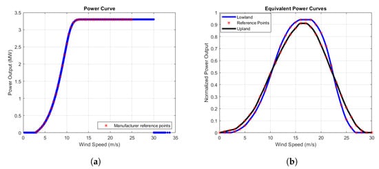
Figure 1.
Two wind power curve models: (a) the Vestas V112-3.3MW wind turbine power curve. (b) the McLean equivalent power curve model.
As shown in Figure 1a, a typical power curve of a single turbine is sigmoid with three distinct breakpoints. The net output of a wind farm is practically zero when the wind speed is below the cut-in level (3 m/s in most cases), reaches its peak (rated power) for wind speeds above 12 m/s and falls back to zero at the cut-out level (30 m/s). In contrast with the classic sigmoid curve of a single wind turbine, the EPC model depicted on Figure 1b is pi- or bell-shaped. A wind farm contains more than one turbine whose rotors typically catch different directions. In extreme wind conditions, turbines are not shut down simultaneously, causing the overall output to gradually drop to zero levels. As the EPC models are more reflective of the real production of a wind farm, we have adopted them in all subsequent stages of our analysis.
4.2. Risk Diversification
Financial markets offer a wide range of investment options varying from traditional securities, such as stocks, bonds and derivatives, to more contemporary tradable financial assets, such as cryptocurrencies. These markets witness a huge amount of transactions daily and continue to grow at an exponential rate. Investment in the above mentioned assets can in periods yield substantial profits to individuals or institutions and contribute to the growth of particular sectors of the economy. However, poorly chosen investment products can lead to significant loses. The relationship between risk and reward is almost universally positively correlated across all investment vehicles. The majority of the investors have a conservative risk profile and would take on extra risk only if compensated with extra return. This fundamental observation is the main driver of Modern Portfolio Theory (MPT) developed by Markowitz in the 1950s [27]. Apart from allocating the available capital in a single asset, constructing a portfolio that efficiently combines a number of securities characterized by uncorrelated returns can yield an improved risk-reward relationship. This property has spurred numerous researchers, including the authors of the present study, to expand the range of application of MPT beyond traditional financial securities; in our case, in the optimal allocation of generation capacity [6,18,20,28,29,30].
The revenue of a wind farm project is subject to uncertainty primarily due to the lack of predictability of winds blowing at its surroundings. The cashflows of such an investment are closely tied to the volume output. A comprehensive and illustrative measure of the efficiency of a power generation system is the capacity factor. This factor is calculated as the ratio of the actual energy output in the operating time period over the maximum amount of energy that would be delivered under ideal weather conditions (which make the farm to produce at power rating levels). In our study, we use daily-averaged wind speed data, thus it makes sense to calculate capacity factors on a daily basis. The (daily) capacity factor is defined as follows:
This asset utilization index is stochastic and ranges between 0 and 100%. In this study, we deal with spatial diversification strategies, i.e., geographical distribution of generating capacity for diversifying away fluctuations in the daily capacity factor of a particular region (grid point) of the Greek mainland. Thus it makes sense to provide a formula for the portfolio daily capacity factor (), which is shown to be a weighted average of the capacity factors of individual grid points
where stands for the proportion of capacity absorbed by grid point and is the cardinality of our asset universe (see [6]). Assessing the production profile of variable energy generating assets involves the calculation of both the mean (denoted as ) and the standard deviation (denoted as ) of the daily capacity factor (across the time dimension). The portfolio’s mean daily generating capacity can be calculated as follows:
where denotes the mean capacity factor of grid point i, is the vector of portfolio weights and ′ is the symbol for the transpose of a matrix. Similarly, we arrange the asset-specific mean capacity factors in the column vector . The portfolio variance can be compactly written in a quadratic form
due to the symmetry property of the variance-covariance matrix , where stands for the covariance of the daily capacity factors of grid points i and j, .
All subsequent portfolio selection exercises will be based on the minimization of the portfolio variance subject to a set of linear constraints
Constraint (5a) states that all of the available capacity has to be distributed among the different assets (full allocation constraint), where denotes the N-dimensional vector of ones. Constraint (5b) sets a target mean capacity factor () for the portfolio. This constraint is removed when calculating the minimum variance (MV) portfolio. If is set equal to , where , the solution of the optimization problem is the maximum yield (MY) portfolio. Constraints (5c) and (5d) (floor and ceiling constraints, respectively) impose lower and upper bounds, respectively, on the share of the total capacity allocated in each grid point, where , , and for all . These constraints are included in the formulation of the portfolio-selection problem to prevent assets from taking disproportionately small or large capacity shares.
After calculating the MV portfolio capacity factor, we can derive the efficient frontier comprising all capacity allocations with an optimal trade-off between yield and risk. In our case, the yield is specified by the mean generating capacity and the risk by the standard deviation of generating capacity. We used a numerical procedure to sample the efficient frontier. The procedure starts with the derivation of the MV capacity allocation and its associated yield (). We then performed a discretization of the closed interval into equidistant points , with boundary conditions and . At each iteration we set the target yield equal to and solve the optimization problem (5).
4.3. Factor Analysis
Wind energy generation is forged by a variety of weather-related effects and seasonality patterns. Specific meteorological phenomena can have a positive or negative impact on the overall production of an individual site or a cluster of wind farms. The investigation of the cross-dependence structure of different locations can pave the way for a site-selection methodology that reduces the uncertainty of wind resources. The output variance of a wind farm or a portfolio of wind farms can be decomposed into two main parts: the systematic component, which includes common sources of variability that have an impact on groups of areas on a national or even broader scale, and the idiosyncratic or non-systematic component, which reflects area-specific atmospheric conditions. The idiosyncratic variance can in principle be mitigated by combining assets with heterogeneous production profiles (although, as we show in [6] and possibly contrary to the tradition investment conviction, the diversification strategy can also be proven effective in eliminating systematic components of risk depending on the sign/size of factor loadings).
Let denote the matrix of capacity factors after apply the logistic transformation, where , T is the sample size, and
Following [6], we assume the following linear factor structure for the transformed capacity factors:
where denotes the T-dimensional vector of ones, the vector of constant terms, the matrix of factor scores (K is the number of latent factors), the matrix of factor loadings and is the matrix of non-systematic components.
A popular technique for estimating a factor model is Principal Component Analysis (PCA). PCA is capable of identifying a limited set of uncorrelated factors, expressed as an affine transformation of the original variables, which are responsible for systematic variations in the generating capacities. Principal components are arranged in a descending order, based on the total amount of variance that they explain. The decision on the optimal number of the common risk components K can be based upon information criteria, such as Bai and Ng [31] or Alessi et al. [32]. Graphical techniques such as the scree plot are also quite popular as they are easy to apply.
4.4. Numerical Weather Prediction Model
This study utilizes numerical simulations performed by the non-hydrostatic Weather Research and Forecasting (WRF) model with the Advanced Research dynamic solver (WRF-ARW v.3.7.1) [33,34,35]. The model is configured with three telescoping nests (one-way) covering most of Europe and North Africa (WRF-D01), central and eastern Mediterranean (WRF-D02), Greece and Asia Minor (WRF-D03), as in Tegoulias et al. [36]. The horizontal resolution for each model domain was 15, 5 and km, respectively, while 39 sigma levels (up to 50 hPa with increased resolution within boundary layer) were deployed in vertical. Gridded ERA-Interim reanalyses ( lat-lon) [37] were used as initial and boundary conditions (every 6 h). This reanalysis dataset has been produced by the European Centre for Medium range Weather Forecasts (ECMWF) using: (a) observations of temperature at 2 m, surface pressure, relative humidity at 2 m and 10 m winds from weather stations, buoys and ships, (b) upper air measurements of temperature, specific humidity and horizontal wind components from radiosondes, wind profilers, aircraft, pilot balloons and (c) data from geostationary and polar-orbiting satellites. The full list of the various data sources of the ERA-Interim reanalyses was provided by [37]. In addition, high-resolution ( lat-lon) Sea Surface Temperatures (SSTs) provided by National Centers for Environmental Prediction (NCEP) were inserted as initial conditions in the model and remained fixed throughout the integration time of each WRF simulation. Fine-resolution data (30 arc s × 30 arc s) of the United States Geological Survey were used for the definition of the WRF topography and land uses. The forecast window was set to 36 h (starting at 12 UTC), with the first 12 h considered as spin-up time. The simulated period spanned from 1 January 2006 to 31 December 2010, while the output from the inner domain (WRF-D03) was saved at hourly intervals.
The Ferrier (Eta) scheme [38] and the Yonsei’s University (YSU) scheme [39] were utilized for the representation of microphysics and boundary layer processes, respectively. Shortwave and longwave radiation were represented by the RRTMG scheme [40], the surface layer processes by the Monin-Obukhov (MM5) scheme, the sub-grid scale convection was parameterized by the Betts-Miller-Janjic scheme [41] (only in the parent and intermediate domains), while the NOAH Unified model [42] was used for land and soil physics. The numerical weather simulations were performed by computational time granted by the Greek Research and Technology Network (GRNET) in the National HPC facility—ARIS—under project PR001009-COrRECT.
4.5. Dataset
From the available 3-D hourly simulated wind speeds of the km native model grid (WRF-D03), a lat-lon grid was produced by using bi-linear interpolation. The hourly wind speed at a height of 120 m was then retrieved by applying linear interpolation between two adjustment vertical levels lying at approximately 85 m and 142 m above the ground, respectively. Finally, the daily mean wind speed at 120 m height was calculated, producing a dataset of total 29,145 grid points at a spatial resolution of lat-lon for each available day. The grid covers Greece from – (latitude) to – (longitude). However, only 5444 points were found to be strictly in between the boundaries of Greek territory and all the rest were excluded from the analysis. Furthermore, we applied a land-sea mask from the WRF model to filter out grid points over the sea, since this study is only about the onshore wind energy resource (5182 grid points). The analyzed period is from 1 January 2006 until 31 December 2010 (due to some technical issues, a small fraction of dates is missing that does not exceed of the sample observations).
The methodologies that will be discussed later on were similarly applied to a second dataset, aiming to both validate and augment the understanding of our findings across different temporal scopes and sample sets, all confined within the geographical boundaries of Greece. To fulfill this purpose, we employed the ERA5 reanalyses [43] dataset as an additional reference sample. This dataset consists of 1353 grid points with daily mean wind speed simulated values at 120 m above ground. The ERA5 data covers the area of – (latitude) and – (longitude) with a spatial resolution of lat-lon. As in the WRF dataset, filtering was also applied to include only the Greek onshore grid points (220 in total). The time period which is covered by the ERA5 are the years 1981–2020. Due to minor differences between the outcomes of the methodologies applied to these two samples, we have made the decision to present the results of the first scenario (based on WRF simulated wind speeds). This selection was primarily motivated by the finer resolution and greater spatio-temporal intricacy provided by the WRF simulation. The outcomes based on ERA5 data are available upon request. All calculations were carried out using MATLAB R2021a.
5. Results
5.1. Descriptive Statistics
As a first step to assessing the wind potential of Greece, an overview of the statistical properties of wind generating capacities is given. To this end, Figure 2a,b provide high-resolution maps of the yield and risk of each grid point, as measured by the mean and the standard deviation of daily capacity factors. For comparison, we also provide an atlas of average wind speeds in Figure 2c. Areas featuring a more intense shade of red have a higher value on the corresponding variable while the white areas are neutral (values are near zero). Locations with extremely high and low values are pin-pointed on the maps to analyze the relationship between generation yield/risk and mean wind speed.
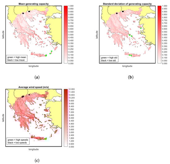
Figure 2.
Spatial assessment of Greek onshore wind resources: (a) mean generating capacity (b) standard deviation of generating capacity (c) average wind speed.
Aegean Sea islands (to the east) and Crete (to the south) have a rich wind profile. This pattern is consistent with the morphological characteristics of the Aegean Basin (wind speeds are high in sites near the sea) and the presence of the Etesian winds (Meltemia) during the summer [44,45,46,47]. Etesian outbreaks tend to have higher density in August, while they present inter-annual variability with a negative trend over the June to September period [48]. Additionally, these outbreaks experience heightened occurrence over elevated terrains such as the Pindos mountain range (to the west) and other lofty landscapes where wind speeds are notably elevated.
The volatility levels shown in Figure 2b are quite similar across all grid points. However, we observe slight changes in the hue that follow the spatial patterns of mean generating capacity. Coastal and mountain areas tend to score higher in terms of and , followed by areas lying in the interior of the topographic polygon. It is noteworthy that the geographical locations associated with the lowest and highest wind speed values are in close proximity but do not always overlap with those characterized by the lowest and the highest mean capacity factor. The EPC model presented in Figure 1b assumes a bell-shaped power curve. This means that extremely low or high wind speed conditions result in relatively low values of generating capacity. As a consequence, areas of almost similar average wind speed profile can have different mean generating capacity. The maps of Figure 2 illustrate that areas of high generation uncertainty do not necessarily match with locations characterized by high mean capacity factor. This is explained again from the shape of the EPC model. The highest generation output is attained for a small range of wind speed values lying in the interior of the power curve domain. Areas characterized by highly fluctuating wind speeds are unlikely to attain an average production near rated power. On the other hand, it seems that extremely low volatility levels typically come with low average power delivery, thus the black dots of the maps generally coincide with each other.
The relationship between wind speed and generating capacity can be further investigated by careful inspection of the energy production distribution (empirical density) of the grid points featuring the lowest and highest mean generating capacity. An area of weak wind potential is expected to have a right-skewed production distribution; zero-production events occur with high frequency, extreme weather phenomena are rare and the generation profile is relatively stable. Such a generation profile is detected in Exaplatanos, a village in the prefecture of Pella, in northern Greece. The histogram of daily-averaged wind speeds and generating capacities, shown in the top panels of Figure 3, confirm the previous claims. The two bottom panels of Figure 3 detail the generation profile of Lasithi, a region in the eastern part of the Crete island. Lasithi has very rich wind resources but this comes with the cost of increased volatility. The distribution of daily-averaged wind speeds and generating capacities are more flattened and allocate mass to a wider range of values. The study of Kotroni et al. [23] revealed a significant reliance of wind potential on the slope of the Greek terrain, rather than solely on the absolute elevation. This observation is somewhat reflected in the wind energy generation distributions depicted in Figure 3 as well as the maps of Figure 2.
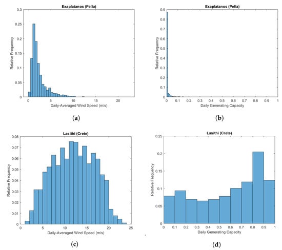
Figure 3.
The wind energy generation profile of the most and least productive regions in Greece. Shown is the distribution of (a) daily-averaged wind speeds in Exaplatanos (b) daily capacity factors in Exaplatanos (c) daily-averaged wind speeds in Lasithi (d) daily capacity factors in Lasithi.
Another compelling aspect of wind energy generation is the positive correlation between yield and risk. Figure 4a shows that the most promising sites in terms of are typically characterized by high levels of production uncertainty, as measured by the standard deviation of daily generating capacities (). This “no-free-lunch property” of the Greek wind resources is especially pronounced in highly productive areas. Figure 4b attempts to shed more light to the “no-free-lunch” finding by showing how the – relationship varies with the altitude of the generation site. Unavoidably high altitude clusters of grid points are thinner, which makes it hard to draw solid conclusions as to the significance of this factor. However, it seems that the altitude does not alter the – pattern which can be eventually attributed to meteorological factors, such as the slope, mountain winds phenomena, the intensity of the pressure systems and fronts that cross the area of interest as well as the logarithmic profile of the wind speed. A further investigation of this topic requires a more in-depth meteorological analysis of the Greek wind field which is out of the scope of this paper.
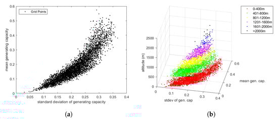
Figure 4.
The risk-yield trade-off of the wind energy generation profile of Greek sites: (a) all grid points. (b) variation with altitude.
The risk-yield trade-off discussed above has important implications for the effectiveness of current energy harvesting practices and the future deployment of wind power plants. It raises a cautionary flag to yield-seeking investors. By prioritizing the commitment of sites with large average capacity factors, investors end up with a more stochastic asset and have limited control on volume risk. Among others, Figure 4a shows that optimal site selection is a non-trivial task that requires a more delegate and multi-faceted evaluation of the generation profile to maintain a balance between yield and risk. The exploration of this observed relationship in the wind field holds promise for revealing valuable insights into weather phenomena. Moreover, it could pave the way for the inception of innovative financial instruments that leverage these insights to secure cash flows.
5.2. Factor Model Estimation
Alessi et al.’s information criterion [32] indicates the existence of common factors in transformed wind generating capacities. In total, the four extracted principal components explain of the data sample variance. Figure 5 presents the scree plot. The horizontal axis enumerates the principal components and the vertical axis measures the percentage of total data variance explained by each factor. The curve exhibits an elbow point after the fourth principal component (as the red line indicates), which is in agreement with the information criterion.
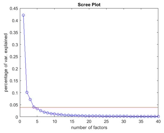
Figure 5.
Scree plot: percentage of total sample variance explained by each factor.
Table 1 presents the percentage and cumulative percentage of variance explained by each common factor. The first common factor holds prominence, as it makes up for a significant amount of the total variance () while the subsequent factors explain relatively smaller percentages.

Table 1.
Sample variance explained by each factor.
The conspicuous commonality observed among the grid points implies a great level of resemblance in the power generation profiles. Following the estimation of principal components, we gauge the exposure of local wind generation profiles to the common risk factors. Three tools are mainly used for that purpose. Figure 6 illustrates how the 5182 grid points are loaded by the most prominent common factors, in the so-called loading maps.
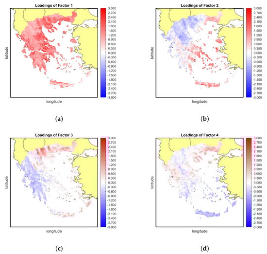
Figure 6.
Loading maps of onshore wind generation sites: (a) Factor 1. (b) Factor 2. (c) Factor 3. (d) Factor 4.
Figure 6a depicts the spatial distribution of factor-1 loadings. Note that all areas are positively exposed to the first principal component, with the coastal areas presenting higher loading values than mountainous ones. This situation hampers the ability to diversify away the first systematic risk component, since there are no grid points that could help offset the positive exposure to factor-1 effects. Therefore, of the variability in wind generation cannot be reduced simply by pooling wind resources. An inspection of the loadings map shows that the first factor incorporates an elevation effect on the variability of the daily wind speeds. As seen in Figure 6a, high-altitude regions (such as the Pindos Mountain ridge to the west) are clearly distinguished from low altitude areas, such as in central Macedonia to the north or Thessaly in central Greece. The rest of the common factors are characterized by loadings of mixed sign leading to a distinctive division of the Greek territory in blue- and red-colored zones. In the case of factor 2, there is a clearly defined border between positively loaded regions (mostly in the south-western Greece) and negatively loaded ones (in the north-eastern Greece). This factor mainly imprints the influence of the Etesian winds, which are in principle highly variable [48]. Constructing a factor-2-neutral portfolio involves pooling areas that exhibit positive and negative exposure to this particular common factor. With proper selection of generating sites, one is able in principle to eliminate the percentage of data variance attributed to factor 2, i.e., approximately . A similar phenomenon is evident for the third factor, albeit with some variations in the orientation of delineated zones. In this case, the blue-colored areas are primarily concentrated in the western and southern parts of Greece, while the red zone extends over the Aegean Sea and also covers the North Greece. This factor contributes an additional to the sample variance, which could be potentially diversified away in a properly selected portfolio with adequate representation of dipolar zones. Progressing further to less eminent factors, the spatial patterns exhibit a decreasing level of definition and no clear associations with topographical or climatic features can be made.
Loadings maps are a static description of the exposure of local generation profiles to systematic risk factors. To provide more insight into temporal patterns imprinted in these risk components, we provide monthly box plots of factor scores. Figure 7 shows how the distribution of factor scores varies across months. The red line marks the position of the median, while the lower and upper side of the boxes correspond to the first and third quantile of the conditional distribution.
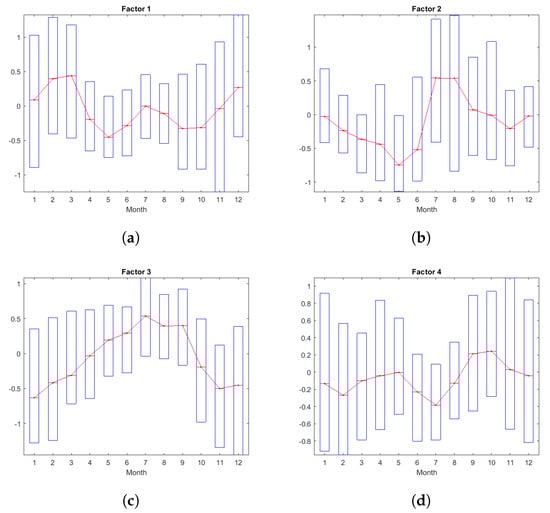
Figure 7.
Monthly box plots of the principal component scores: (a) Factor 1. (b) Factor 2. (c) Factor 3. (d) Factor 4.
Monthly distributions unveil distinctive patterns of seasonality in wind power generation. Seasonality is not only evident in the median but also in the dispersion of values. Specifically, factor 1 scores tend to be higher and more volatile during winter months and at the beginning of the spring season. The first principal component may be reflective of the general atmospheric circulation during this season, when low pressure systems accompanied by high wind speeds prevail over Greece. The second factor follows a slightly different pattern. It imprints regions whose median wind energy supply experiences an upshoot during July and August, accompanied by higher levels of wind generation uncertainty. This factor appears to be reflective of the inter-annual variability associated with the Etesian winds, mostly influencing areas along the Aegean Sea coast. The intricate interactions between these wind patterns and seasonal changes contribute to the observed patterns in wind power generation and its associated variability across different months. The third factor follows a clear ascending trend starting from January and ending in August. After August, its scores undergo a significant reduction albeit with increasing temporal fluctuations. The volatility pattern resembles that of the first factor, with lower dispersion of values in summer and higher dispersion of values in winter and spring, in line with the trends previously identified. Lastly, the fourth factor lacks a distinctive pattern. Its influence appears to be associated with relatively less significant weather effects, as indicated by the loading map’s non-uniform displacement of color zones. There is a minor peak observed during the autumn season and volatility remains lower in summer but comparatively higher across all other seasons of the year. Different factor patterns underscore the complexity of wind power generation’s dependence on multiple weather-related variables and the intricate interactions among them.
The combined inspection of loading maps and monthly box plots provides a comprehensive depiction of the wind power generation profile of each geographical area. The final generation output derived from the factor model results from the multiplication of loadings and factor scores, where the sign of the loading determines the overall impact of a factor on the area’s energy generation. For instance, the first factor captures an increase in the wind energy production across all onshore sites during the winter months. Coastal areas, characterized by higher loading estimates, will experience a more substantial trend. The second factor yields a distinctly different effect across the two color zones. Positively loaded locations (red areas) are expected to witness an increase in daily generation in July and August, whereas those with negative loading coefficients will observe decreased production during the same period. This observation underscores the benefit of including locations with mixed-sign loadings in a generation portfolio. The patterns for the third and fourth factor closely resemble each other. In areas of positive loading, higher factor scores lead to an increase in output, whereas negatively loaded (blue) sites exhibit a decrease in production with higher factor scores.
A final aspect of the risk factor dynamics we consider is the autocorrelation structure. The degree of autocorrelation provides insight into how a sudden disturbance in factor scores is propagated into the regional production levels on subsequent days. A high level of autocorrelation suggests that a systematic generation shock will have a persistent effect on regional energy production. On the other hand, a low degree of autocorrelation indicates that temporary disturbances in wind energy generation tend to fade away more quickly having a short-term impact on local production.
Figure 8a shows the sample autocorrelation function (SACF) of factor-1 scores. Also depicted is a significance envelope. Autocorrelation coefficient estimates exhibit an oscillating pattern and are significantly statistically different than zero even at distant lags. This suggests that shocks in the first factor are particularly persistent, with disturbances tending to dissipate slowly. Moving to the second factor, Figure 8b illustrates a consistent and rapid decay in the autocorrelation after the fifth lag but shocks tend to persist until the 12th lag, being indicative of a more prolonged effect. Factor 3 is probably the most persistent; in the SACF of Figure 8c, autocorrelation coefficient estimates lie above the upper significance bound at all lags. On the contrary, factor 4 exhibits shorter memory as indicated by the existence of significant autocorrelation mostly up to the 5th order (see Figure 8d).
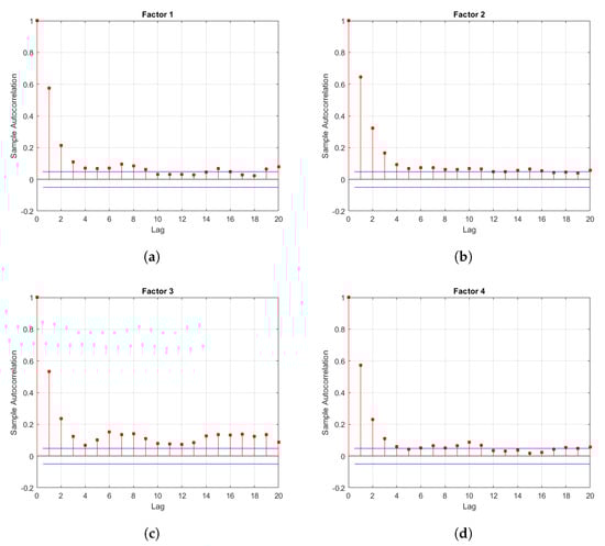
Figure 8.
Sample autocorrelation functions of common risk factors: (a) Factor 1. (b) Factor 2. (c) Factor 3. (d) Factor 4.
5.3. PCA and Area Selection
In the previous section, we presented the main statistical properties of the common principal components. To gain a better understanding of how each factor additively contributes to the forging of local generation profiles, we performed a reconstruction analysis. The gradual incorporation of each factor results in an immediate transformation of the generation schema over time, thereby facilitating the identification of each risk component. Given the extensive cross-section of our sample, we analyze the loadings patterns of three distinctive areas, shown in the maps of Figure 9 (black boxes). They are located in Chios Island to the east ( lat, lon), the city of Giannitsa in northern Greece ( lat, lon) and the island of Corfu to the west ( lat, lon). The Chian site has a strong positive exposure to the second factor and a weak positive exposure to the third factor. The site near Giannitsa, on the other hand, demonstrates a medium negative exposure to the second factor and a medium positive exposure to the third factor. Lastly, the selected area on Corfu has a moderate negative exposure to both second and third factor. The monthly averaged (transformed) generation profile of these three assets is anticipated to change with the incorporation of each factor. In fact, each principal component can be conceived as a building block that adds to the complexity of the local generation profile. This property is illustrated in a series of box plots (see Figure 10, Figure 11 and Figure 12).

Figure 9.
Factor loadings on selected areas: (a) Factor 1. (b) Factor 2. (c) Factor 3. (d) Factor 4.
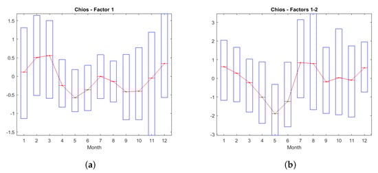
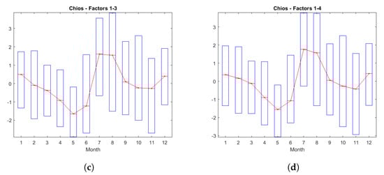
Figure 10.
The incremental wind energy generation profile of a site in Chios: (a) Factor 1. (b) Factor 2. (c) Factor 3. (d) Factor 4.
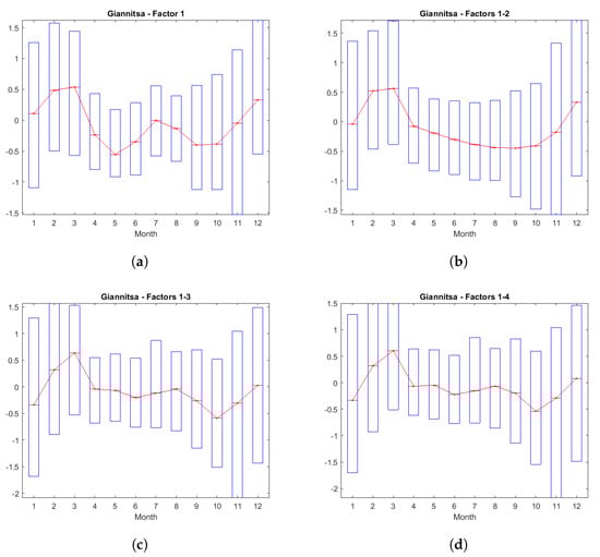
Figure 11.
The incremental wind energy generation profile of a site in Giannitsa: (a) Factor 1. (b) Factor 2. (c) Factor 3. (d) Factor 4.
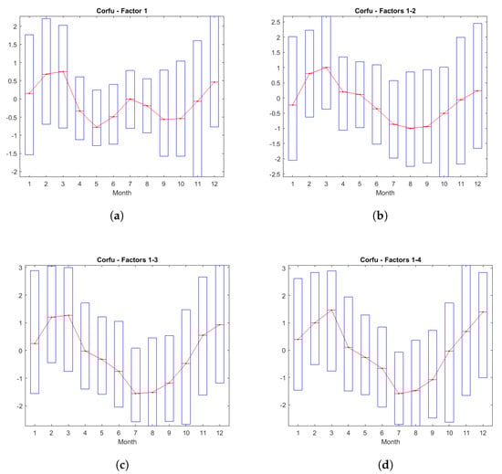
Figure 12.
The incremental wind energy generation profile of a site in Corfu: (a) Factor 1. (b) Factor 2. (c) Factor 3. (d) Factor 4.
Figure 10a shows that for the reference grid point on Chios, factor 1 shapes the baseline production profile (also presented in Figure 7). The incorporation of the second factor in the model introduces a noticeable decline in the generation output during the spring season, coupled with a leap in generation in July and August (see Figure 10b). This observation suggests that the Etesian winds (discussed in [48]) exert significant influence on the area’s production profile in the last two summer months with an overall positive impact. From an inspection of Figure 10c,d we conclude that the third factor does not significantly alter the main patterns, except for a minor decline in the wind energy supply in winter months, and the fourth factor slightly enhances the production in July. Overall, the second factor has the most important contribution to the forging of the local generation profile for the selected Chian site, clearly imprinting Etesian wind effects which are particularly pronounced in this insular region of Greece in the summer season.
As the box plots of Figure 11 suggest, the grid point of Giannitsa has a completely different generation profile than Chios. As in the previous case, the first factor sets the baseline (amounting to relatively elevated generation in winter and early spring months), The second principal component maps the descending trend in wind energy supply as we move from the winter to the summer season. This is in sharp contrast to the local generation profile of the Chian site, where production reaches its maximum in July and August. The declining trend in generation levels is characterized by relatively low sample variability. The third factor contributes to a more uniform monthly distribution of the transformed capacity factor, by slightly increasing production in the spring and the summer season. This finding is explained by the positive loading of factor 3 on this site. Figure 11d does not support the existence of a significant seasonal pattern in the contribution of this factor.
Figure 12 shows factor incremental effects for the case of the Corfiot site. The first principal component contributes in a similar way, but factor 2 infuses a pattern that is mirror opposite to that observed in the Chian site. The addition of the second factor imposes a decline in the monthly generating capacity in spring and summer, accompanied by increased levels of volatility. This is indicative of the the variability of the wind speeds prevailing over Corfu during these months, since both synoptic (e.g., front passages) and thermodynamic conditions (e.g., thunderstorms) affect the wind field. The third factor amplifies the impact of the second factor, leading to a further decline in average production. As for the fourth factor, it only implants a minor peak in production levels during March, with no substantial alteration of the overall generation profile.
5.4. The Minimum Variance Portfolio
Generation portfolio were selected in the quadratic optimization framework discussed in Section 4.2. Our asset universe is composed of candidate areas for wind power harvesting. As many as 50 portfolios were found enough to attain a good level of approximation to the efficient frontier, starting from the minimum variance and ending to the maximum yield portfolio. Figure 13 presents the efficient frontier along with the – coordinates of individual grid points (black dots) and efficient assets (yellow dots). The latter are the grid points that are used in any efficient capacity allocation plan. Efficient assets are in total 35, after omitting locations that absorb less than of the overall available capacity in any efficient portfolio. Remarkably, with only 35 out of the 5182 available grid points, one can attain the optimal trade-off between generation risk and yield for any yield target set by the decision maker. This is evident of the great deal of redundancy in the asset universe but also the possibility of detecting regions that act as good substitutes to others (the latter is important whenever the selected site is not available for wind energy harvesting due to land usage (urban, environmental) restrictions). Also depicted in Figure 13 is the equally weighted (EW) capacity allocation and two more portfolios (EWS and EWM) that present efficient alternatives to the equally weighted one across the and axis, respectively.
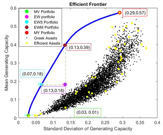
Figure 13.
A – analysis of alternative wind energy harvesting plans.
The MV portfolio reserves only nine areas (receiving weight ) for wind energy harvesting. The spatial distribution of generating capacity dictated by this plan is presented in Figure 14. Most of the available capacity goes to three sites in the municipality of Almopia (prefecture of Pella) to the north. One of them is the dominant asset of the portfolio absorbing of the total installed capacity. The other two assets absorb in total (% and ) of the portfolio’s capacity. Xanthi (Thrace) to the northeast has a capacity share of . The remaining is distributed among the Tzoumerka mountains (prefecture of Ioannina) to the northwest, Peloponnese (Tsakonas) to the southwest, Central Macedonia (Kerkini’s lake, near Serres) to the north and Crete (Agia Paraskevi, prefecture of Rethymno and Ierapetra, prefecture of Lasithi) to the south. Most of the grid points picked by the MV portfolio are on mountain terrains and only two of them are close to the Cretan coast. With this pool of regions, the MV capacity allocation manages to bring the standard deviation of the daily capacity factor down to the remarkable level of , greatly reducing the uncertainty of the aggregate output of the wind farm network. Despite this improvement in the reliability of the aggregate wind energy generation, the MV portfolio has a poor mean output level (the average daily capacity factor is only ). This trade-off between risk and yield highlights one of the shortcomings of the MV portfolio-selection approach: seeking to lower volatility, one ends up with a wind energy harvesting plan that attains a poor utilization rate of the available resources. This calls into question the practical value of implementing such a capacity allocation plan. However, owing to the relative steepness of the efficient frontier near the MV edge, we are in principle able to boost the average delivered output with a tolerable increase in volume risk. For instance, the EWS portfolio depicted on Figure 13 manages to rise the mean wind utilization rate to , which is times higher than the MVP’s, with an increase in the day-to-day variability by a factor of only.
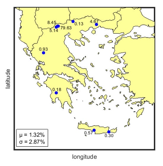
Figure 14.
The minimum variance spatial allocation of wind generating capacity.
5.5. Portfolio Evaluation
Following [6], we assess the diversification benefits of the minimum variance portfolio through the Risk Reduction (RR) index defined as follows:
where denotes the standard deviation of the MV portfolio capacity factors and asset i’s risk. Figure 15a shows the RR ability of the MV portfolio for each grid point and efficient asset. The latter locations were picked by the MV procedure primarily due to their low volume risk levels as well as their weak correlation structure. An intriguing observation is that the efficient assets are distributed throughout Greece, spanning both mountainous and coastal regions. Many grid points are situated within the mountain range of Pindos (to the west) while others are found on the island of Crete (to the south). In particular, the eastern and southern regions of Crete are more suitable due to the complex terrain of the island which results in gap winds and wind flow acceleration as documented in [23,49]. Each of the efficient assets possesses a unique wind profile ideal for wind farm installations. For instance, in the summer season, coastal areas tend to experience higher wind speeds, while in the winter, wind speeds are elevated in the mountainous regions. This explains why both types of areas are combined in efficient portfolios.
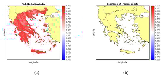
Figure 15.
Risk reduction index per (a) grid point and (b) efficient asset.
As Figure 15a shows, the risk reduction is substantial for the great majority of grid points, being indicative of the inefficiency or redundancy of most areas in Greece when it comes to wind energy harvesting. High RR index values are also observed across efficient assets, which shows that only through the pooling of generating sites we are able to competently manage volume risk. Only three points have an RR in the range 0– and these locations have the highest share of allocated capacity in the MV portfolio.
In addition to the risk reduction ability discussed earlier, there are other criteria that warrant consideration before finalizing the optimal capacity allocation plan. An essential aspect to analyze is the risk exposure of the MV portfolio to common risk factors. While diversification aims to reduce the idiosyncratic risk component by selecting areas with different generation profiles, it is possible that systematic factors may still introduce instability into the portfolio’s generation. To address this concern, Figure 16 projects the MV solution on loading maps. Green-colored boxes mark the nine locations reserved by the MV portfolio, also discussed in Section 5.4. If the locations designated by the portfolio exhibit risk factor loadings that are numerically close to zero or loadings of mixed signs, this indicates that these factors can indeed be eliminated through the pooling of resources. It is evident that the first risk factor cannot be diversified away as all loadings are of the same sign (positive). In an attempt to reduce the production volume fluctuations attributed to this factor, the MV portfolio has chosen areas of relatively low exposure. Figure 16b shows that the MV portfolio reserves harvesting sites of mixed sign in an attempt to control or even neutralize the effect of the second common risk component. The same pattern is also observed for the third factor as six areas are located in the red and the rest in the blue zone (see Figure 16c). Factor 4 is diversifiable as well, given that the portfolio-designated areas feature mixed exposures to this risk component, indicated by the varied loadings.
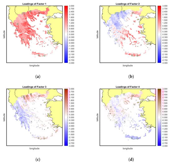
Figure 16.
Factor loadings on the MV portfolio: (a) Factor 1. (b) Factor 2. (c) Factor 3. (d) Factor 4.
In Section 5.7, we apply PCA to decompose the generation risk of the MV portfolio. Low percentages will indicate a neutralization of a specific risk factor while the opposite will be indicative of persistence.
5.6. Efficient Portfolios
The MV solution has been found to yield a suboptimal generation output, making it impractical for implementation in a real-world scenario. Nevertheless, given the steepness of the efficient frontier, alternative portfolios warrant consideration in determining the final spatial allocation plan. To assess these alternatives, Figure 17 depicts the empirical distribution of the wind energy capacity factor for six representative efficient capacity allocations, including the MV and the MY. The MY plan allocates of the available capacity in the southeastern corner of Crete. Portfolios are numbered in increasing order of mean generating capacities (), where portfolio n.1 coincides with the MV and portfolio n.50 with the MY capacity allocation. The exact position of the selected capacity allocation plans on the efficient frontier is shown in Figure 18b.
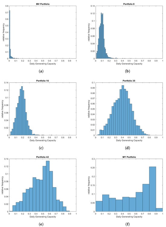
Figure 17.
The daily generating capacity distribution of six portfolios on the efficient frontier. (a) MV. (b) portfolio n.8. (c) portfolio n.16. (d) portfolio n.35. (e) portfolio n.42. (f) MY.
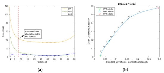
Figure 18.
(a) CV and percentage change in and across the efficient frontier. (b) The position of selected portfolios on the efficient frontier.
The histograms of Figure 17 reveal an interesting property of the wind energy production distribution of efficient portfolios. All capacity allocations near the lower edge of the efficient frontier have a left-skewed production distribution, the asymmetry being particularly pronounced in the case of the MV portfolio. Moving towards the middle of the efficient frontier, specifically in portfolios with a mean generating capacity of –, the distribution of daily capacity factors gradually becomes more symmetric (elliptical). This finding can be attributed to the weighting of the portfolio-selection objectives. To minimize the risk level, the algorithm efficiently locks in a small number of locations characterized by mild wind conditions. However, when the goal is also to boost generation output, the algorithm moves to areas of richer wind profiles, even if this results in an increasing variability of the capacity factor.
The adoption of a MV capacity allocation leads to a high number of zero-generation days, rendering the wind harnessing plan unproductive. On the other hand, portfolio n.50 (MY) may not be a viable option due to its high generation uncertainty. Portfolios whose numbering ranges between 16 and 35 present a more acceptable compromise, as they help mitigate excessive variability while offering higher average power delivery. To make a well-informed decision, it is advisable to examine these portfolios in detail, taking into account factors such as the number of selected assets, technical barriers in wind farm installation, alignment with the existing environment and urban planning regulations. By considering these aspects, an investor can identify the portfolio that offers the best balance between risk and generation output while being conducive to practical implementation.
Figure 19 shows the daily evolution of the capacity factor for the designated portfolios of the efficient frontier and Figure 20 provides the monthly box plot of the corresponding time series. An inspection of the time plots verifies that both the mean and variance levels of the generating capacity have significant dissimilarity along the efficient frontier. For instance, the MV portfolio displays multiple clusters of near-zero production days, resulting in a lower risk level. Conversely, the MY portfolio demonstrates the opposite trend with higher mean generation but also more fluctuations in the daily output level.
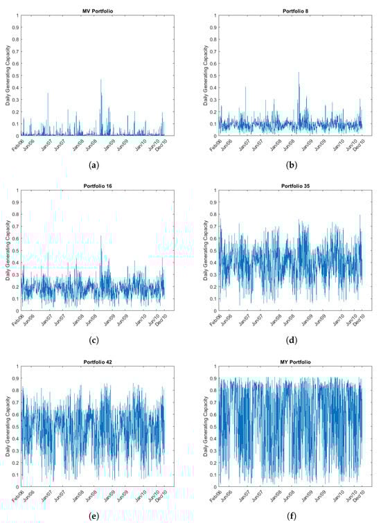
Figure 19.
The evolution of the daily capacity factor for six representative portfolios of the efficient frontier: (a) MV. (b) portfolio n.8. (c) portfolio n.16. (d) portfolio n.35. (e) portfolio n.42. (f) MY.
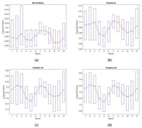
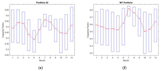
Figure 20.
A seasonality analysis of daily capacity factors for six portfolios of the efficient frontier: (a) MV. (b) portfolio n.8. (c) portfolio n.16. (d) portfolio n.35. (e) portfolio n.42. (f) MY.
The box plots reveal that in all portfolio cases the daily generation tends to peak during the summer season. The winter season is also quite productive, while in spring and autumn the output of the interconnected array of wind farms decreases. This seasonal pattern becomes more pronounced as we move from the MV to the MY capacity allocation plan. The generation variability differs across seasons. Winter, marked by extreme weather conditions, exhibits significantly higher wind speed variability. In contrast, in the summer, the daily dispersion of capacity factors is lower. In the subsequent section, we will perform a factor analysis of the portfolios power delivery to explore the sources of variability, dissect wind generation risk and evaluate the results of the optimization process.
An approach that can be easily applied to facilitate the selection of the favorable spatial allocation plan is to calculate the percentage increase in risk and yield as we trace up the sequence of efficient portfolios. The percentage incremental risk is defined by , where for . The associated relative difference in average generation output is given by . The results of this analysis are depicted in Figure 18a. We also show the evolution of the coefficient of variation , measuring the trade-off between average generation output and volume risk in each efficient portfolio. The lower the CV, the more favorable the relationship between and becomes.
Figure 18a illustrates an important property of efficient wind capacity allocations. In the lower segment of the efficient frontier (almost up until portfolio n.10), the percentage gain in terms of is much higher compared to the relative increase in . This property enables the aggregator to significantly improve the average power delivery while holding volume risk at acceptable levels. The CV decreases rapidly as we trace up the efficient frontier and reaches its lowest value () at portfolio n.33. The CV curve is relatively flat near the minimum, meaning that one can attain similar risk and yield trade-offs with a wide range of portfolios lying in the interior of the efficient frontier. Surprisingly, all curves become near flat at the vicinity of the eighth portfolio, which means that this capacity allocation could be a reasonable alternative to the MV solution, as it offers much higher mean generating capacity while efficiently controlling volatility levels. The spatial capacity distribution of this portfolio is depicted in Figure 21a. Blue dots show the selected locations and the labels close to the dots designate the percentage of available capacity absorbed by each site. Figure 21b, to the right, pictures an efficient alternative to the equally-weighted capacity allocation, i.e., the portfolio on the efficient frontier that offers the same mean generating capacity with EW. The two illustrated portfolios have many assets in common with the MV solution but also include additional locations. The efficient EW portfolio reserves a total of 17 areas and portfolio n.8 includes 16 assets. The spatial capacity distribution dictated by both plans is quite similar in terms of geographical expansion and participation of climatic zones.
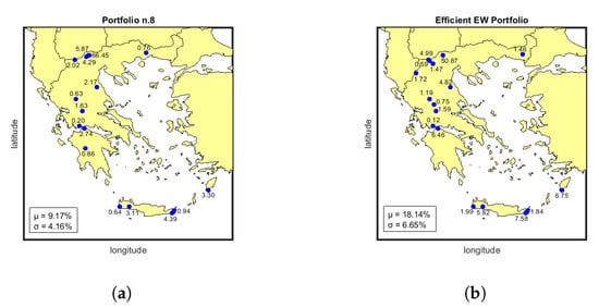
Figure 21.
Two efficient wind capacity allocation plans: (a) portfolio n.8. (b) the efficient equally weighted portfolio.
5.7. Risk Decomposition of Efficient Portfolios
As a final step in the evaluation of efficient capacity allocation plans, we measure the exposure of each portfolio to the systematic risk components. The estimated loading of factor , , on portfolio P is , where is the loading of factor k on asset i and is the capacity share of asset i in the portfolio. Based on the sample properties of loading and factor estimates, we are able to perform a decomposition of the portfolio’s sample variance as
where stands for the portfolio’s systematic risk component.
Table 2 reports the percentage variance decomposition of the (transformed) portfolio capacity factors. The last two columns show the relative shares of the systematic and the idiosyncratic components. The power output of all efficient portfolios is largely shaped by the first factor, with the exception of the MY portfolio which reserves a single site in the southeastern tip of Crete. This outcome is verified by the loadings map of Figure 6a. The risk contribution of other common factors is also significant in certain capacity allocations. The variance decomposition analysis reveals that the MV portfolio output has the lowest exposure to the common risk factors. As shown in Figure 16, the MV portfolio holds positions that are not much loaded by the first factor and also have mixed (positive and negative) exposure to other risk components. An inspection of the sixth column of Table 2 indicates that the systematic variance share increases as we trace up the efficient frontier, meaning that the optimization procedure has focused on mostly eliminating common sources of risk by holding sites residing on dipolar zones. The MY portfolio deviates from this trend; as a single-site harvesting plan, its generation profile is largely idiosyncratic.
Table 2.
Percentage risk decomposition of efficient portfolios.
6. Conclusions and Future Research
The primary goal of this empirical study was to examine the wind energy generation profile of onshore Greek regions and analyze the possibility of reducing volume risk through the pooling of resources. Experimental results indicate that coastal areas and mountain ranges possess rich wind profiles albeit with elevated variability. Typically, high productivity is associated with increasing generation uncertainty, a finding which we call “no free lunch”, and is also observed in other terrains (see also [6]). The no-free lunch property of Greek wind resources has two important implications. First, it suggests that it is generally not possible to improve power delivery without taking on additional volume risk. Secondly, it makes imperative to consider a risk management strategy that could improve the average utilization of wind energy resources while placing a limit on volume risk.
Due to the unavailability of financial instruments or insurance products that could hedge away volume risk (at least the financial consequences of it), we unavoidably restrict attention to diversification strategies. These amount to pooling resources by forming an array of interconnected wind power generation sites, whose collective output could be traded as a unified asset. To evaluate the effectiveness of this strategy to diversify away volume risk, we analyze the covariance structure of grid points with the aid of principal components analysis. PCA identified the existence of four systematic risk components that are collectively responsible for of the daily generation variance. These components induce a rich spatial covariance structure in the Greek wind energy field. The first factor makes up for of the total sample variance and is non-diversifiable, as it loads all regions by the same sign. Although of systematic origin, the remaining common components have a mixed effect on the production profile of each region and can be diversified away in a properly selected portfolio. Common factors have a strong seasonal signature and incorporate weather phenomena of the northeastern Mediterranean, like the Etesian winds.
After analyzing the covariance structure, we applied quadratic programming techniques to derive the Pareto set of spatial capacity allocation plans that attain the optimal trade-off between generation yield and risk. Remarkably, an exceptionally small fraction of grid points (35 out of 5182) constitute the basis of all Pareto-optimal portfolios. This finding sends a sound message to regulators about the importance of the smart selection of generation sites and it generally suggests that it is possible to integrate large amounts of wind energy to the power grid without employing a large scale commitment of regions for wind power harnessing. Another pivotal result underscores that the minimum variance portfolio is highly inefficient; due to the steepness of the lower segment of the efficient frontier, there exist alternative portfolios with a substantially improved average utilization factor and controllable volume risk levels. Furthermore, a great range of portfolios along the efficient frontier have a comparable coefficient of variation offering relatively stable mean generating capacity per unit of volume risk. A subsequent decomposition of aggregate generation profiles revealed that most efficient portfolios manage to diversify away regional generation risk although maintaining a large exposure to systematic risk components, particularly factor 1. This underscores the necessity of exploring alternative strategies to hedge away (financially or physically) this source of generation uncertainty.
Despite the valuable insights gained from this study, it is crucial to acknowledge limitations affecting interpretation and generalization of the findings. First, our study employs simulated capacity factors to quantify volume risk and derive various statistics of the production distribution. While offering certain advantages over actual generation data, simulated capacity factors have several weaknesses. They rest on models (weather models or power curves) to accurately reflect the wind power generation potential of a region. Portfolio optimization is sensitive to mean and covariance estimates, with adverse implications for the robustness of efficient portfolios. Although applied to transformed capacity factors, PCA performs a linear decomposition of generation risk. Devising a nonlinear factor model is a non-trivial task adding a layer of complexity to the interpretation of results.
The efficient management of renewable energy resources is a contemporary topic that has gained prominence in academic literature in recent years and remains an open field for future research. There are several pathways along which our study could be expanded. Deriving optimal harvesting plans utilizing mixed-technology generating units could be of strategic significance for Greece due to its rich wind and solar resources. The combination of wind and solar power plants in a single array has shown to enhance and stabilize the generation profile in many cases due to the complementary property of these resources [30,50,51]. Furthermore, marine energy, such as wave and tidal, could be part of an integrated portfolio [52]. Offshore areas could be also incorporated in the asset universe, as Greece possesses a great number of small rock islands that are away from urban regions and present themselves as good options for wind power harvesting [53,54].
Another direction of future research is the consideration of hedging strategies to mitigate the wind volume risk. Wind power futures and similar derivative assets are ideal for financially mitigating volume risk and securing the income of wind power producers and aggregators [6,7,55,56,57]. Although such products are constantly gaining attention in the investment community, they are still unavailable for Greece. Our study has the potential to stimulate research in this direction and pave the way for the development of new derivatives designed to capture various dimensions of volume risk [6,58].
Author Contributions
Conceptualization, N.S.T.; Methodology, N.S.T.; Software, N.S.T., T.C., S.K. and I.P.; Validation, N.S.T. and T.C.; Formal analysis, N.S.T. and T.C.; Investigation, N.S.T. and T.C.; Resources, T.C., S.K. and I.P.; Data curation, T.C., S.K. and I.P.; Writing—original draft, N.S.T., T.C., S.K. and I.P.; Supervision, N.S.T. and I.P.; Project administration, N.S.T. All authors have read and agreed to the published version of the manuscript.
Funding
The numerical weather simulations were performed by computational time granted by the Greek Research and Technology Network (GRNET) in the National HPC facility—ARIS—under project PR001009-COrRECT.
Data Availability Statement
Data are available upon request.
Conflicts of Interest
The authors declare no conflict of interest.
Abbreviations
The following abbreviations are used in this manuscript:
| CV | Coefficient of Variation |
| EPC | Equivalent Power Curves |
| MPT | Modern Portfolio Theory |
| MV | Minimum Variance |
| MY | Maximum Yield |
| PCA | Principal Component Analysis |
| RES | Renewable Energy Sources |
| SACF | Sample Auto Correlation Function |
| WRF | Weather Research and Forecasting |
References
- Androniceanu, A.; Sabie, O. Overview of Green Energy as a Real Strategic Option for Sustainable Development. Energies 2022, 15, 8573. [Google Scholar] [CrossRef]
- Geden, O.; Schenuit, F. Climate Neutrality as Long-Term Strategy: The EU’s Net Zero Target and Its Consequences for Member States. 2019. Available online: https://www.ssoar.info/ssoar/handle/document/63951 (accessed on 30 November 2023).
- Sheikhahmadi, P.; Bahramara, S. The participation of a renewable energy-based aggregator in real-time market: A Bi-level approach. J. Clean. Prod. 2020, 276, 123149. [Google Scholar] [CrossRef]
- Kleidon, A. Physical limits of wind energy within the atmosphere and its use as renewable energy: From the theoretical basis to practical implications. arXiv 2020, arXiv:2010.00982. [Google Scholar] [CrossRef]
- Kaufmann, J.; Kienscherf, P.A.; Ketter, W. Modeling and managing joint price and volumetric risk for volatile electricity portfolios. Energies 2020, 13, 3578. [Google Scholar] [CrossRef]
- Thomaidis, N.S.; Christodoulou, T.; Santos-Alamillos, F.J. Handling the risk dimensions of wind energy generation. Appl. Energy 2023, 339, 120925. [Google Scholar] [CrossRef]
- Christensen, T.S.; Pircalabu, A. On the spatial hedging effectiveness of German wind power futures for wind power generators. J. Energy Mark. 2018, 11, 71–96. [Google Scholar] [CrossRef]
- Archer, C.L.; Jacobson, M.Z. Evaluation of global wind power. J. Geophys. Res. Atmos. 2005, 110, 110.D12. [Google Scholar] [CrossRef]
- Holttinen, H. Hourly wind power variations in the Nordic countries. Wind. Energy Int. J. Prog. Appl. Wind. Power Convers. Technol. 2005, 8, 173–195. [Google Scholar] [CrossRef]
- Archer, C.L.; Jacobson, M.Z. Supplying baseload power and reducing transmission requirements by interconnecting wind farms. J. Appl. Meteorol. Climatol. 2007, 46, 1701–1717. [Google Scholar] [CrossRef]
- Kempton, W.; Pimenta, F.M.; Veron, D.E.; Colle, B.A. Electric power from offshore wind via synoptic-scale interconnection. Proc. Natl. Acad. Sci. USA 2010, 107, 7240–7245. [Google Scholar] [CrossRef]
- Handschy, M.; Rose, S.; Apt, J. Reduction of wind power variability through geographic diversity. arXiv 2016, arXiv:1608.06257. [Google Scholar]
- Cassola, F.; Burlando, M.; Antonelli, M.; Ratto, C.F. Optimization of the regional spatial distribution of wind power plants to minimize the variability of wind energy input into power supply systems. J. Appl. Meteorol. Climatol. 2008, 47, 3099–3116. [Google Scholar] [CrossRef]
- McQueen, D.; Wood, A. Quantifying benefits of wind power diversity in New Zealand. IET Renew. Power Gener. 2019, 13, 1338–1342. [Google Scholar] [CrossRef]
- Santos-Alamillos, F.; Pozo-Vázquez, D.; Ruiz-Arias, J.; Lara-Fanego, V.; Tovar-Pescador, J. A methodology for evaluating the potential contribution of wind energy to baseload power: A case study in Andalusia (Southern Spain). Renew. Energy 2014, 69, 147–156. [Google Scholar] [CrossRef]
- Grothe, O.; Schnieders, J. Spatial dependence in wind and optimal wind power allocation: A copula-based analysis. Energy Policy 2011, 39, 4742–4754. [Google Scholar] [CrossRef]
- Thomaidis, N.S. Designing strategies for optimal spatial distribution of wind power. In Proceedings of the 5th International Scientific Conference on Energy and Climate Change, Athens, Greece, 11–12 October 2012. [Google Scholar]
- Roques, F.; Hiroux, C.; Saguan, M. Optimal wind power deployment in Europe—A portfolio approach. Energy Policy 2010, 38, 3245–3256. [Google Scholar] [CrossRef]
- Reichenberg, L.; Johnsson, F.; Odenberger, M. Dampening variations in wind power generation—The effect of optimizing geographic location of generating sites. Wind. Energy 2014, 17, 1631–1643. [Google Scholar] [CrossRef]
- Santos-Alamillos, F.; Thomaidis, N.; Usaola-García, J.; Ruiz-Arias, J.; Pozo-Vázquez, D. Exploring the mean-variance portfolio optimization approach for planning wind repowering actions in Spain. Renew. Energy 2017, 106, 335–342. [Google Scholar] [CrossRef]
- Novacheck, J.; Johnson, J.X. Diversifying wind power in real power systems. Renew. Energy 2017, 106, 177–185. [Google Scholar] [CrossRef]
- Musselman, A.; Thomas, V.M.; Boland, N.; Nazzal, D. Optimizing wind farm siting to reduce power system impacts of wind variability. Wind. Energy 2019, 22, 894–907. [Google Scholar] [CrossRef]
- Kotroni, V.; Lagouvardos, K.; Lykoudis, S. High-resolution model-based wind atlas for Greece. Renew. Sustain. Energy Rev. 2014, 30, 479–489. [Google Scholar] [CrossRef]
- Wagner, R.; Antoniou, I.; Pedersen, S.M.; Courtney, M.S.; Jørgensen, H.E. The influence of the wind speed profile on wind turbine performance measurements. Wind. Energy Int. J. Prog. Appl. Wind. Power Convers. Technol. 2009, 12, 348–362. [Google Scholar] [CrossRef]
- Gottschall, J.; Peinke, J. How to improve the estimation of power curves for wind turbines. Environ. Res. Lett. 2008, 3, 015005. [Google Scholar] [CrossRef]
- McLean, J. WP2. 6—Equivalent Wind Power Curves; TradeWind: Madrid, Spain, 2008; Volume 2. [Google Scholar]
- Markowitz, H.M. Portfolio selection. In Portfolio Selection; Yale University Press: New Haven, CT, USA, 1968. [Google Scholar]
- Geem, Z.W.; Kim, J.H. Optimal energy mix with renewable portfolio standards in Korea. Sustainability 2016, 8, 423. [Google Scholar] [CrossRef]
- Hu, J.; Harmsen, R.; Crijns-Graus, W.; Worrell, E. Geographical optimization of variable renewable energy capacity in China using modern portfolio theory. Appl. Energy 2019, 253, 113614. [Google Scholar] [CrossRef]
- Santos-Alamillos, F.; Pozo-Vazquez, D.; Ruiz-Arias, J.A.; Von Bremen, L.; Tovar-Pescador, J. Combining wind farms with concentrating solar plants to provide stable renewable power. Renew. Energy 2015, 76, 539–550. [Google Scholar] [CrossRef]
- Bai, J.; Ng, S. Determining the number of factors in approximate factor models. Econometrica 2002, 70, 191–221. [Google Scholar] [CrossRef]
- Alessi, L.; Barigozzi, M.; Capasso, M. Improved penalization for determining the number of factors in approximate factor models. Stat. Probab. Lett. 2010, 80, 1806–1813. [Google Scholar] [CrossRef]
- Skamarock, W.C.; Klemp, J.B.; Dudhia, J.; Gill, D.O.; Barker, D.M.; Duda, M.G.; Huang, X.Y.; Wang, W.; Powers, J.G. A description of the advanced research WRF version 3. NCAR Tech. Note 2008, 475, 113. [Google Scholar]
- Wei Wang, C.; Duda, M.; Dudhia, J.; Gill, D.; Kavulich, M.; Keene, K.; Chen, M.; Lin, H.; Michalakes, J.; Rizvi, S.; et al. ARW Version 3 Modeling System User’s Guide; NCAR: Boulder, CO, USA, 2016. [Google Scholar]
- Powers, J.G.; Klemp, J.B.; Skamarock, W.C.; Davis, C.A.; Dudhia, J.; Gill, D.O.; Coen, J.L.; Gochis, D.J.; Ahmadov, R.; Peckham, S.E.; et al. The weather research and forecasting model: Overview, system efforts, and future directions. Bull. Am. Meteorol. Soc. 2017, 98, 1717–1737. [Google Scholar] [CrossRef]
- Tegoulias, I.; Kartsios, S.; Pytharoulis, I.; Kotsopoulos, S.; Karacostas, T.S. The influence of WRF parameterisation schemes on high resolution simulations over Greece. In Proceedings of the 13th International Conference of Meteorology, Climatology and Atmospheric Physics, Thessaloniki, Greece, 19–21 September 2016; Perspectives on Atmospheric Sciences. Springer: Berlin/Heidelberg, Germany, 2017; pp. 3–8. [Google Scholar]
- Dee, D.P.; Uppala, S.M.; Simmons, A.J.; Berrisford, P.; Poli, P.; Kobayashi, S.; Andrae, U.; Balmaseda, M.; Balsamo, G.; Bauer, D.P.; et al. The ERA-Interim reanalysis: Configuration and performance of the data assimilation system. Q. J. R. Meteorol. Soc. 2011, 137, 553–597. [Google Scholar] [CrossRef]
- Rogers, E.; Black, T.; Ferrier, B.; Lin, Y.; Parrish, D.; DiMego, G. Changes to the NCEP Meso Eta Analysis and Forecast System: Increase in resolution, new cloud microphysics, modified precipitation assimilation, modified 3DVAR analysis. NWS Tech. Proced. Bull. 2001, 488, 15. [Google Scholar]
- Hong, S.Y.; Noh, Y.; Dudhia, J. A new vertical diffusion package with an explicit treatment of entrainment processes. Mon. Weather. Rev. 2006, 134, 2318–2341. [Google Scholar] [CrossRef]
- Iacono, M.J.; Delamere, J.S.; Mlawer, E.J.; Shephard, M.W.; Clough, S.A.; Collins, W.D. Radiative forcing by long-lived greenhouse gases: Calculations with the AER radiative transfer models. J. Geophys. Res. Atmos. 2008, 113. [Google Scholar] [CrossRef]
- Janjić, Z.I. The step-mountain eta coordinate model: Further developments of the convection, viscous sublayer, and turbulence closure schemes. Mon. Weather. Rev. 1994, 122, 927–945. [Google Scholar] [CrossRef]
- Tewari, M.; Chen, F.; Wang, W.; Dudhia, J.; LeMone, M.; Mitchell, K.; Ek, M.; Gayno, G.; Wegiel, J.; Cuenca, R.H. Implementation and verification of the unified NOAH land surface model in the WRF model (Formerly Paper Number 17.5). In Proceedings of the 20th Conference on Weather Analysis and Forecasting/16th Conference on Numerical Weather Prediction, Seattle, WA, USA, 10–12 January 2004; Volume 14. [Google Scholar]
- Hersbach, H.; Bell, B.; Berrisford, P.; Hirahara, S.; Horányi, A.; Muñoz-Sabater, J.; Nicolas, J.; Peubey, C.; Radu, R.; Schepers, D.; et al. The ERA5 global reanalysis. Q. J. R. Meteorol. Soc. 2020, 146, 1999–2049. [Google Scholar] [CrossRef]
- Hochman, A.; Alpert, P.; Harpaz, T.; Saaroni, H.; Messori, G. A new dynamical systems perspective on atmospheric predictability: Eastern Mediterranean weather regimes as a case study. Sci. Adv. 2019, 5, eaau0936. [Google Scholar] [CrossRef]
- Dafka, S.; Akritidis, D.; Zanis, P.; Pozzer, A.; Xoplaki, E.; Luterbacher, J.; Zerefos, C. On the link between the Etesian winds, tropopause folds and tropospheric ozone over the Eastern Mediterranean during summer. Atmos. Res. 2021, 248, 105161. [Google Scholar] [CrossRef]
- Dafka, S.; Toreti, A.; Zanis, P.; Xoplaki, E.; Luterbacher, J. Twenty-first-century changes in the Eastern Mediterranean Etesians and associated midlatitude atmospheric circulation. J. Geophys. Res. Atmos. 2019, 124, 12741–12754. [Google Scholar] [CrossRef]
- Dafka, S.; Xoplaki, E.; Toreti, A.; Zanis, P.; Tyrlis, E.; Zerefos, C.; Luterbacher, J. The Etesians: From observations to reanalysis. Clim. Dyn. 2016, 47, 1569–1585. [Google Scholar] [CrossRef]
- Tyrlis, E.; Lelieveld, J. Climatology and dynamics of the summer Etesian winds over the eastern Mediterranean. J. Atmos. Sci. 2013, 70, 3374–3396. [Google Scholar] [CrossRef]
- Koletsis, I.; Lagouvardos, K.; Kotroni, V.; Bartzokas, A. The interaction of northern wind flow with the complex topography of Crete Island–Part 1: Observational study. Nat. Hazards Earth Syst. Sci. 2009, 9, 1845–1855. [Google Scholar] [CrossRef]
- Monforti, F.; Huld, T.; Bódis, K.; Vitali, L.; D’isidoro, M.; Lacal-Arántegui, R. Assessing complementarity of wind and solar resources for energy production in Italy. A Monte Carlo approach. Renew. Energy 2014, 63, 576–586. [Google Scholar] [CrossRef]
- Thomaidis, N.S.; Santos-Alamillos, F.J.; Pozo-Vázquez, D.; Usaola-García, J. Optimal management of wind and solar energy resources. Comput. Oper. Res. 2016, 66, 284–291. [Google Scholar] [CrossRef]
- Jahanshahi, A.; Kamali, M.; Khalaj, M.; Khodaparast, Z. Delphi-based prioritization of economic criteria for development of wave and tidal energy technologies. Energy 2019, 167, 819–827. [Google Scholar] [CrossRef]
- Bagiorgas, H.S.; Mihalakakou, G.; Rehman, S.; Al-Hadhrami, L.M. Offshore wind speed and wind power characteristics for ten locations in Aegean and Ionian Seas. J. Earth Syst. Sci. 2012, 121, 975–987. [Google Scholar] [CrossRef]
- Spyridonidou, S.; Vagiona, D.G.; Loukogeorgaki, E. Strategic planning of offshore wind farms in Greece. Sustainability 2020, 12, 905. [Google Scholar] [CrossRef]
- Benth, F.E.; Benth, J.Š. Dynamic pricing of wind futures. Energy Econ. 2009, 31, 16–24. [Google Scholar] [CrossRef]
- Benth, F.E.; Di Persio, L.; Lavagnini, S. Stochastic modeling of wind derivatives in energy markets. Risks 2018, 6, 56. [Google Scholar] [CrossRef]
- Benth, F.E.; Christensen, T.S.; Rohde, V. Multivariate continuous-time modeling of wind indexes and hedging of wind risk. Quant. Financ. 2021, 21, 165–183. [Google Scholar] [CrossRef]
- Yamada, Y.; Matsumoto, T. Construction of Mixed Derivatives Strategy for Wind Power Producers. Energies 2023, 16, 3809. [Google Scholar] [CrossRef]
Disclaimer/Publisher’s Note: The statements, opinions and data contained in all publications are solely those of the individual author(s) and contributor(s) and not of MDPI and/or the editor(s). MDPI and/or the editor(s) disclaim responsibility for any injury to people or property resulting from any ideas, methods, instructions or products referred to in the content. |
© 2024 by the authors. Licensee MDPI, Basel, Switzerland. This article is an open access article distributed under the terms and conditions of the Creative Commons Attribution (CC BY) license (https://creativecommons.org/licenses/by/4.0/).