Article

Optimization of Financial Indicators in Shale-Gas Wells Combining Numerical Decline Curve Analysis and Economic Data Analysis

1
Group of Numerical Methods in Engineering—GMNI, Center for Technological Innovation in Construction and Civil Engineering—CITEEC, Civil Engineering School, Universidade da Coruña, Campus de Elviña, 15071 A Coruña, Spain
2
Department of Civil Engineering: Hydraulics, Energy and Environment, Universidad Politécnica de Madrid, 28006 Madrid, Spain
3
Department of Civil and Environmental Engineering, Massachusetts Institute of Technology, Cambridge, MA 02139, USA
4
Department of Earth, Atmospheric and Planetary Sciences, Massachusetts Institute of Technology, Cambridge, MA 02139, USA
*
Author to whom correspondence should be addressed.
Energies 2024, 17(4), 864; https://doi.org/10.3390/en17040864
Submission received: 7 December 2023 / Revised: 30 January 2024 / Accepted: 4 February 2024 / Published: 12 February 2024

Abstract

:
We present a methodology to determine optimal financial parameters in shale-gas production, combining numerical simulation of decline curves and stochastic modeling of the gas price. The mathematical model of gas production considers free gas in the pore and the gas adsorbed in kerogen. The dependence of gas production on petrophysical parameters and stimulated permeability is quantified by solving the model equations in a 3D geometry representing a typical fractured shale well. We use Monte Carlo simulation to characterize the statistical properties of various common financial indicators of the investment in shale-gas. The analysis combines many realizations of the physical model, which explores the variability of porosity, induced permeability, and fracture geometry, with thousands of realizations of gas price trajectories. The evolution of gas prices is modeled using the bootstrapping statistical resampling technique to obtain a probability density function of the initial price, the drift, and the volatility of a geometric Brownian motion for the time evolution of gas price. We analyze the Net Present Value (NPV), Internal Rate of Return (IRR), and Discounted Payback Period (DPP) indicators. By computing the probability density function of each indicator, we characterize the statistical percentile of each value of the indicator. Alternatively, we can infer the value of the indicator for a given statistical percentile. By mapping these parametric combinations for different indicators, we can determine the parameters that maximize or minimize each of them. We show that, to achieve a profitable investment in shale-gas with high certainty, it is necessary to place the wells in extremely good locations in terms of geological parameters (porosity) and to have exceptional fracturing technology (geometry) and fracture permeability. These high demands in terms of petrophysical properties and hydrofracture engineering may explain the industry observation of “sweet spots”, that is, specific areas within shale-gas plays that tend to yield more profitable wells and where many operators concentrate their production. We shed light on the rational origin of this phenomenon: while shale formations are abundant, areas prone to having a multi-parameter combination that renders the well profitable are less common.

1. Introduction

The shale-gas production line is very broad [1,2,3], from gas extraction through the well (upstream) and gathering, storing and transformation of the gas (midstream), to the distribution and transportation of gas to households and industry (downstream) [4,5,6,7]. Several engineering processes along this complex value chain are well-suited for the implementation of optimization techniques that may improve the overall system efficiency [8,9,10]. These include the optimization of fracturing fluid properties, gas transport processes, and geometric design of the shale-gas wells, among others [11,12,13,14,15]. Here, we focus on financial optimization of the shale-gas wells using financial indicators like Net Present Value (NPV), Internal Rate of Return (IRR), and Discounted Payback Period (DPP) [16,17,18,19,20,21,22,23,24,25,26]. A novelty of our approach is that we consider uncertainty in gas prices. We refer to the financial optimization of shale-gas wells as the search for the petrophysical and well parameters that maximize or minimize a percentile of a certain financial indicator [27,28,29]. These objective functions allow us to find the optimal parameters for a certain level of risk. This information helps in making more informed decisions [30,31,32,33,34,35].
In this study, we seek to determine the values of the design parameters of a shale-gas well and the geological characteristics of a shale-gas reservoir that maximize or minimize the financial indicators NPV, IRR, and DPP for a certain probability of occurrence [36,37,38]. We adopt as our main uncertain parameters the porosity of the formation, the permeability induced by hydraulic fracturing, and the geometry of the fractured reservoir volume (known as Effective Propped Volume, EPV), assuming that these three parameters are the most relevant for methane production and shale-gas financial performance [39,40,41,42,43,44,45]. We neglect the variability in other parameters, such as distance between fractures along the well, or the amount of kerogen in the source rock [46,47,48,49]. The distance between hydraulic fractures does not have a relevant impact on financial indicators since the cost of executing a shale-gas well is essentially determined by the number of hydraulic fractures and the length of the fractured wells. The position of the hydraulic fractures does not change the execution cost significantly. In relation to gas production, the distance between hydraulic fractures can affect the production speed, although not so much the accumulated production over 10 years. Thus, if the fractures are very close to each other, production interference will occur very early, causing the production regime to go from potential decay (slow) to exponential decay (fast). But when all the interference is fully developed between the fractures, the regime will again be potential, and the long-term production will be very similar regardless of the position of the fractures. This will mean that the influence on the NPV or the IRR will be low, and the indicator that may be somewhat altered would be the DPP given that the speed of gas production determines the rate of recovery of the investment. On the other hand, kerogen, in the case studied in this article, has adsorption properties that mean that the gas produced by this source is very low. For the amount of gas produced to be relevant, the pressure would have to drop a lot, a phenomenon that does not occur. Therefore, for the purposes of cash flows derived from gas from kerogen, we can consider them little relevant and without influence on the financial indicators.
The conceptual approach that we propose in this work is novel in that we seek to determine parameters that optimize financial indicators that have a certain probability of occurrence. Explained with two examples, we determine the values of porosity, induced permeability, and geometry of the EPV that maximize the NPV whose probability of occurrence is 90% or higher, or the parametric set that minimizes the DPP whose probability of occurrence is 60% or less. We chose these probability thresholds because they are the ones that will give us results of the financial indicators within the parameter values that would be common in shale-gas exploitation, e.g., porosity between 1% and 5%. The use of Discounted Payback Period (DPP), or the time required for an investment to be amortized from an economic point of view, is also a novelty of this work.
The proposed methodology combines numerical simulation of gas production and stochastic simulation of the gas price based on historical data. Through computational fluid dynamics, we obtain the decline curves of gas production for different combinations of porosity ( ϕ ), induced permeability or EPV permeability ( k E P V ), and EPV geometry values (AR) [50,51,52]. Using historical gas price data and applying the bootstrapping statistical re-sampling technique [53], we obtain the drift and volatility of the stochastic process of gas price evolution over time [54]. We then use Monte Carlo simulation [55] to generate thousands of possible gas price trajectories over a 10-year time period. These trajectories are combined with the production decay curves, obtaining multiple values of the NPV, IRR, and DPP financial indicators. We fit a probability density function (PDF) using the Gaussian Kernel Density Estimation method (KDE) [56]. Finally, for each percentile and for parametric combination ( ϕ , k, AR) we perform a calculation of the value of the financial indicators, generating a field of iso-probability curves on which the optimization calculations will be carried out by a scanning technique.
The proposed optimization process is applied to a prototype shale well. The main conclusion of this study is that, to achieve a positive investment (NPV > 0 and IRR > 0) with low recovery time (DPP), very demanding and therefore rare geological and design parameter combinations are required; that is, high porosities, very high induced permeabilities, and very flat fracture geometries. Our results may help constrain shale-gas reserve calculations [57,58,59] and are consistent with the “sweet spot” theory [60,61,62], which rationalizes the observed phenomenon that shale-gas plays have developed following a geographic pattern of concentration of wells at a few geographic zones within large formations. In these zones, poorly understood characteristics result in profitable investments. With this study, we shed some light on this phenomenon.

2. Materials and Methods

The development of this section presents the methodologies used and the numerical calculations carried out to achieve the objectives set out in the article: optimization of financial indicators in shale-gas investments with statistical percentile quantification. In this sense, the numerical calculations of gas production and the stochastic and statistical process for determining the synthetic series of the gas price are considered intermediate results, which are not the central objective of discussion in this article. The results that are subject to analysis and discussion are all those related to the optimization results. In these, parametric maps are obtained by optimization that determine the values of the NPV, IRR, and DPP for a percentile.

2.1. Physical, Mathematical, and Numerical Model of Gas Production in a Standard Shale-Gas Well

The modeling setup is that of a prototype shale-gas well (Figure 1a) [39,40]. The well depth is 3000 m, and there are seven hydraulic fractures along the 1500 m of the horizontal section of the well. The mathematical model that describes the phenomenon of reservoir pressure evolution and gas flow after hydrofracturing is based on mass conservation for a representative volume of fractured porous medium (Figure 1a) and is derived below.
Mass conservation of gas within a 3D volume can be expressed mathematically as:
m ( x , t ) t = Q ( x , t ) Ω F ( x , t ) Γ ,
where m ( x , t ) is the mass at point x and time t, Q denotes sources and sinks, and F is the mass flux in and out of the volume centered around x . In this study, we assume a single-component gas (methane), neglecting the presence of other light hydrocarbons (e.g., butane). The consideration of multi-component gases does not alter the methodology proposed in this document, but nevertheless, it would make the explanation and calculation developments of the article more complex by having to include a compositional study of the gas and a determination of the viscosity and density of mixing and creating a series of prices for the mix based on the prices of each of the components. All these calculations would delve into already known concepts and would partially cover up the main scientific innovations of this study.
Free gas is present in the pore space and in the form of adsorbed gas in the kerogen. We neglect gas that may be present in other forms, such as dissolved gas in the kerogen. Thus, the total mass of gas for a differential volume (dV) is the sum of free and adsorbed methane. Using the notation of Table 1, the mass differential is:
d m = d m f r e e + d m a d s o r b e d = ρ ϕ d V + ρ 0 ρ k S k V a d V .
Possible unit conversions in the above expression can be analyzed as:
k g C H 4 = k g C H 4 m C H 4 free 3 · m pore 3 m bulk 3 · m bulk 3 + k g C H 4 m C H 4 n. c. 3 · k g kerogen m kerogen 3 · m kerogen 3 m bulk 3 · m C H 4 n. c. 3 k g kerogen · m bulk 3 , k g C H 4 = k g C H 4 free + k g C H 4 adsorbed ,
where we assume that free methane gas occupies all the available pore space so that m C H 4 f r e e 3 = m p o r e 3 .
The integral form of the mass conservation equation can be written as:
t Ω d m = Ω Q d V Γ F n ¯ d Γ .
Neglecting sources and sinks, introducing Equation (2) in Equation (4), and with the parameters and notation of Table 1, Equation (4) reduces to:
t Ω ρ ϕ + ρ 0 ρ k S k V a d V = Γ F n ¯ d Γ .
Applying the divergence theorem and assuming that the control volume does not change in time, Equation (5) can be written as:
Ω t ρ ϕ + ρ 0 ρ k S k V a d V + Ω · F d V = 0 .
The differential form of the mass conservation equation is derived through the Localization Principle, which states that, if the integral form is true for an arbitrary control volume, then the differential form must also hold. Specifically:
I f Ω Ψ ( x , t ) d V = 0 , Ω , t Ψ ( x , t ) = 0 Ω , t ,
which implies that Equation (6) can be written as:
Ω t ρ ϕ + ρ 0 ρ k S k V a + · F d V = 0 .
and mass conservation of free and adsorbed gas in a geological formation is described by:
t ρ ϕ + ρ 0 ρ k S k V a + · F = 0 .
To calculate the flux F , we use Darcy’s law:
F = k ρ μ P ,
so that Equation (9) reads:
t ρ ϕ + ρ 0 ρ k S k V a + · k ρ μ P = 0 .
We use an ideal gas equation of state model for methane that assumes a linear relationship between density and pressure:
ρ = c g P .
The time derivative of the Langmuir isotherm can be written as:
V a t = V a P · P t = c f · P t .
Finally, introducing Equations (12) and (13) into Equation (11), we arrive at the following expression:
c g ϕ + ρ 0 ρ k S k c f P x , t t + c g k μ · P x , t P x , t = 0 ; x Ω Γ a n d t > 0 .
The strong form of the mathematical problem governing the evolution of gas pressure in the reservoir includes Equation (14), supplemented with suitable boundary and initial conditions:
α P x , t t + β · P x , t P x , t = 0 , x Ω Γ a n d t > 0 ,
α = c g ϕ + ρ 0 ρ k S k c f , β = c g k μ ,
P x , 0 = P r x Ω Γ , P x , t = P b h p x Γ a n d t > 0 ,
V a ( P ) = V L P x , t P L + P x , t .
Equations (15)–(18) allow us to calculate the evolution of the field pressure, P x , t , in a 3D domain Ω and in a contour Γ for each point x = ( x , y , z ) , and at each instant of time t. V a ( P ) represents the amount of gas adsorbed by using the mathematical model of the Langmuir isotherm. The meaning and values of the other variables and parameters in Equations (15)–(18) are shown in Table 1 and in [39].
Equation (15) is mass conservation equation that governs the entire computational domain. Coefficients α and β are defined in Equation (16). We obtain these coefficients from the petrological parameters of the hydraulic fractured formation and the PVT properties of the methane. The compressibility factor of the gas is derived from the ideal gas law under isothermal conditions.
Equation (17) defines the initial and boundary conditions of the mathematical formulation. An initial condition of constant pressure is established throughout the domain, Ω , and a Dirichlet-type boundary condition of pressure is imposed on the contours of the well, Γ , where the gas flow out of the formation occurs.
Finally, Langmuir’s isotherm has been included in the mathematical model in order to accurately represent the adsorption phenomenon, Equation (18). In this expression, the Langmuir pressure and the Langmuir volume take values that appear in Table 1 [39] and that have been obtained from [14].
The methane flow rate is calculated from the evolution of the field pressures using, as an integral over the well’s area Γ :
q ( t ) = Γ 2 c g k μ P x , t P x , t · n ¯ d Γ .
Rewriting Equations (15)–(19) in a more compact form, the mathematical model that describes gas production in a shale-gas well appears as:
α P t + · c g k μ P P = 0 ,
α = c g ϕ + ρ 0 ρ k S k c f ,
P x , 0 = P r i n Ω , P x , t = P b h p i n Γ ,
V a = V L P P L + P ,
q ( t ) = Γ 2 c g k μ P P · n ¯ d Γ .
Table 1 shows the meaning of the variables and constants of Equations (20)–(24).
The porosity is assumed to be constant in time, homogeneous, and isotropic for each parametric sweep performed. Likewise, the permeabilities of the EPVs and fractured shale are considered constant, homogeneous, and isotropic regardless of the parameter combination. We discretize and solve the model Equations (20)–(24) using the finite element implementation platform COMSOL Multiphysics ® 5.4 [63]. The computational mesh comprises 155,561 linear tetrahedral elements. The problem domain is a rectangular prism with permeability ranging from 10 18 m 2 to 10 17 m 2 (1 μ D to 10 μ D) [64,65,66,67]. This permeability range in the volumetric domain is chosen for each set of parameters. The Effective Propped Volumes around each planar fracture have an ellipsoidal shape, and their permeability range is 2 × 10 15 m 2 . That is, the model has two permeabilities in each parametric combination: that of the unchanged fractured volume of the EPVs and that of the shale-gas volume domain. For purely comparative purposes, relative to the effect of hydraulic fracturing, we consider that the initial permeability of the shale rock is 10 21 m 2 , equivalent to 1 nano Darcy (nD).
We simulate 10 years of gas flow for different values of porosity, permeability, and flatness of the fracture. Porosities range between 1% and 5%, induced permeabilities between 1 and 10 micro Darcy ( μ D), and fracture flatness between 150 m and 250 m of the semi-major axis of the fracturing ellipsoid. The volume enclosed by these ellipsoids is the same for all parameter combinations and equal to the volume of an ellipsoid of 150 m × 20 m × 35 m (volume = 4.4 × 10 5 m 3 ). Flatness is achieved by keeping this volume and the length of the vertical semi-axis constant while increasing the length of the semi-axis perpendicular to the well and horizontal with respect to the ground. In Figure 1, we present this entire gas production setup.

2.2. Methods for the Statistical Characterization of Financial Indicators

In this section, we explain the combined application of four mathematical/numerical methodologies that allow us to statistically characterize financial indicators of shale well performance.
While the evolution of gas production is determined by the physical model described in the previous section, the evolution of gas price is considered as a stochastic process. Gas price trajectories are modeled as Geometrical Brownian Motions (GBMs) [68,69,70]. To derive the GBM model, we start from an Itô-type stochastic differential equation [71,72,73], particularized for the gas price, P g a s , as:
d P g a s = μ P g a s ( t ) d t + σ P g a s ( t ) d B ( t ) ,
d B t = ξ ( 0 , 1 ) ( t ) d t ,
P g a s ( 0 ) = P 0 .
In Equations (25)–(27), P g a s ( t ) is the value of the gas price at time t, d P g a s is the differential increase of said price in the time interval dt, μ is the drift or general trend of the price of gas, and σ is the gas price volatility or dispersion of normalized price returns.
d B t is an increase in the value of the gas price that follows a Wiener or Brownian motion process, a particular case of a stochastic Markov process [74]. In a Markov process, the probability that a certain event occurs depends solely on the value of the event at the previous instant of time. This mathematical approach fits very well with the Efficient Market Hypothesis [75] in its weak form, according to which the price of an asset (gas in this case) contains in a moment of time t all the information that can affect the value of the asset, with a certain variability or random component that has to do with unexpected news that happens in a chaotic way and that the market cannot discount immediately. In the case of the Wiener process, it is also postulated what the statistical variability of the gas price is. Specifically, the price of gas is considered to have a stochastic component of mean 0 and variance dt.
A Wiener process [76] has mean 0 and variance dt, so the stochastic component of gas price variation can be rewritten in such a way that d B t = ξ ( 0 , 1 ) ( t ) dt , where ξ ( 0 , 1 ) is a normal random distribution with mean 0 and variance 1 that takes independent values in for each time step dt, also called the white noise distribution [77].
To solve solution stochastic differential Equations (25)–(27), we apply Itô’s lemma which, in its full version, can be written as follows [78]: let x(t) be a stochastic process that satisfies the following differential equation with the following initial condition:
d x ( t ) = F ( t , x ( t ) ) d t + g ( t , x ( t ) ) d B ( t ) , t 0 ,
x ( 0 ) = x 0 ,
and F ( x , t ) is a function F: R × [0,T] R such that the following partial derivatives exist and are continuous:
F ( x , t ) t = F 1 ( t , x ) , F ( x , t ) x = F 2 ( t , x ) , F 2 ( x , t ) x 2 = F 22 ( x , t ) .
Then, it can be stated that t > 0 is fulfilled:
F ( x ( t ) , t ) F ( x 0 , s ) = 0 t F 1 ( x ( r ) , r ) + f ( x ( r ) , r ) F 2 ( x ( r ) , r ) d r + 0 t 1 2 ( g ( x ( r ) ) , r ) 2 + F 22 ( x ( r ) , r ) d r + 0 t ( g ( x ( r ) ) , r ) F 2 ( x ( r ) , r ) d B ( r ) .
Writing the Equation (25) in integral form, the following is obtained:
0 t d P g a s ( r ) = 0 t μ P g a s ( r ) d r + 0 t σ P g a s ( r ) d B ( r ) , P g a s ( t ) P g a s ( 0 ) = 0 t μ P g a s ( r ) d r + 0 t σ P g a s ( r ) d B ( r ) .
As P g a s ( t ) is the stochastic variable assimilable to x ( t ) in Itô’s lemma, the following identifications are made:
f ( t , x ( t ) ) = f ( t , P g a s ( t ) ) = μ P g a s ( t ) , g ( t , x ( t ) ) = g ( t , P g a s ( t ) ) = σ P g a s ( t ) , F ( t , x ) = ln ( x ) .
According to the formulations that appear in (30):
F 1 ( t , x ) = F ( t , x ) t = 0 , F 2 ( t , x ) = F ( t , x ) x = 1 x , F 22 ( t , x ) = F 2 ( t , x ) x 2 = 1 x 2 .
Substituting Equations (32)–(34) in the expression of Itô’s lemma (31), we obtain:
ln ( P g a s ( t ) ) ln ( P g a s ( 0 ) ) = 0 t 0 + μ P g a s ( r ) 1 P g a s ( r ) d r + 0 t 1 2 ( σ P g a s ( r ) ) 2 1 P g a s 2 ( r ) d r + 0 t ( σ P g a s ( r ) 1 P g a s ( r ) d B ( r ) .
Simplifying Equation (35), we obtain:
ln P g a s ( t ) P g a s ( 0 ) = 0 t μ 1 2 σ 2 d r + 0 t σ d B ( r ) ,
ln P g a s ( t ) P g a s ( 0 ) = μ 1 2 σ 2 t + σ B ( t ) B ( 0 ) .
The general thesis is that, for t = 0, a Brownian motion type Wiener process takes value 0, that is to say, B(0) = 0. Taking into account this hypothesis, Equation (37) can be solved, and we obtain:
P g a s ( t ) = P g a s ( 0 ) · e [ ( μ 1 2 σ ) t + σ B ( t ) ] , B ( t ) = ξ ( 0 , 1 ) ( t ) t .
In Equation (38), the parameter μ is the drift or trend of the process, σ is the volatility of the gas, and ξ t is a white noise-type random process with distribution ξ t N ( 0 , 1 ) . A price value P 0 is used to calculate gas price P t at the instant t. With this equation, we can simulate random gas price trajectories that meet the behavioral properties of an asset in a perfect market.
We use Equations (39) and (40) to determine the drift and volatility based on the gas price history data. In these equations, P i is the price of gas at the instant i, P i 1 is the price of gas at the instant i−1, Δ t is the time step between two natural gas price observations, and N is the number of observations considered to carry out the estimate. Both expressions come from the application of the Maximum Likelihood Estimation to the estimate of the parameters ( μ , σ ) in a GBM-type stochastic model.
μ ^ = 1 N · Δ t i = 1 N P i P i 1 1 ,
σ ^ = 1 N · Δ t i = 1 N P i P i 1 1 μ ^ Δ t 2 .
.
We can simplify Equations (39) and (40) because there is a temporary data series for gas price at a daily frequency, and the time step considered to estimate the parameters ( μ , σ ) is 1 day; therefore, Δ t = 1 . Likewise, we can understand the expression inside the sum of Equation (39) as the return of the day-to-day gas price normalized to a unit basis. That is, this expression states the gas price increase or decrease over time expressed on a unit basis. Based on these considerations, we rewrite Equations (39) and (40) as Equations (41)–(43).
P i P i 1 1 = R i ,
μ ^ = 1 N i = 1 N R i ,
σ ^ = 1 N i = 1 N R i μ ^ 2 .
The Maximum Likelihood Estimation for drift and volatility can be used to simulate the gas price using GBM. These are simply the arithmetic mean of gas price unitary returns and its standard deviation for a time series of price data with N values.
We simulate gas price trajectories over 10-year periods using GBM, considering that both drift and volatility are variables at each time step. Thus, the initial price, the drift, and the volatility are random variables whose Probability Density Function (PDF) [79] arises from statistical resampling of the historical data series. We take as reference daily gas prices the Henry Hub Spot Price (HHSP) [80] from January 1997 to April 2020.
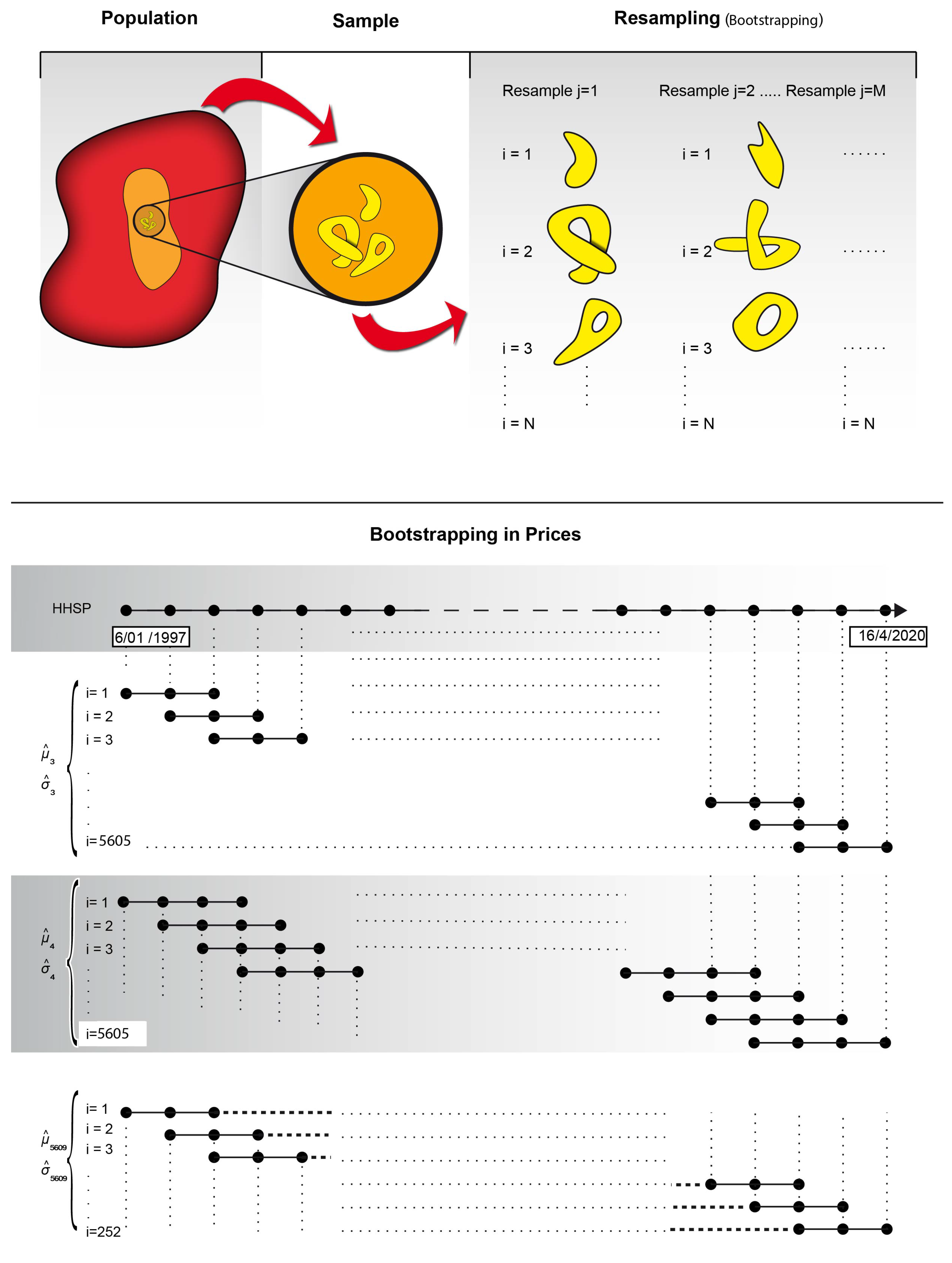
We calculate the empirical initial price, drift, and volatility using a statistical resampling technique known as bootstrapping [53], which aims at improving the accuracy of estimators based on small sample sizes by “resampling the sample”. A subset of N data is taken from the initial sample, and the statistical calculation under investigation is performed using the subset. The data are selected randomly and with replacement, i.e., the data selected are not separated from the original sample but returned to the same, and hence each element can be repeated in the subsample. This operation is repeated M times, with N data taken from the original sample each time. In this manner, we obtain a statistical distribution of the indicator under investigation. This statistical approach is schematically illustrated in Figure 2.
We incorporate some additional considerations regarding the process of calculating the initial price, empirical drift, and volatility based on the HHSP price series:
Each subsample takes a time lapse of between 3 and 5609 days, in such a manner that each of the subsamples consists of consecutive gas price values throughout the historical series of time lapses of 3 days, 4 days, 5 days, etc. The maximum time lapse we take is 5609 days, as this is the equivalent of the historical sample 5861 minus one stock market year of 252 days. Then, for a time lapse of 5609 days, the size or total resamples will be 252, which is considered the reasonable minimum required to generate a probability distribution of a statistic.
The shorter the time lapse, the greater the number of resamples for this time lapse and vice versa.
Each time lapse will generate subsamples with elements that are not repeated and are consecutive over time. In this manner, for two subsamples from a specific time lapse, some of the elements of the subsamples will be repeated twice, at most.
The idea of taking consecutive data over time from the different subsamples comes from the perspective that there is a certain time correlation within the gas price data. It is common to find weak long-tailed or long-term correlations in historical evolution of listed assets [81].
We carry out bootstrapping resampling with time lapses ranging from 3 days to 5609 days. We determine the statistics of drift and volatility of gas prices. For each time lapse, we calculate the empirical probability distribution function for drift and volatility. Furthermore, we carry out a Kolmogorov–Smirnov (K–S) test [82] to determine if the proposed function is rejected or not as a PDF function. Note that no parametric classical functions such as the normal, log-normal, or Weibull distributions are well-suited to fit the empirical distribution function of drift and/or volatility for any studied time lapse. Instead, both statistics are modeled using nonparametric functions consisting of Gaussian kernels. This methodology is known as Kernel Density Estimation or KDE [83], which adapts to empirical frequency distributions with complex data geometries.
We carry out a general analysis, sweeping the entire historical price series for all of the aforementioned time lapses. We look for the time lapse that produces the highest level of significance for both drift and volatility. The significance level provides a metric for how good the adjustment between the theoretical function and empirical function is. The significance level ranges between 0% and 100%, with the common required minimum being 5%.
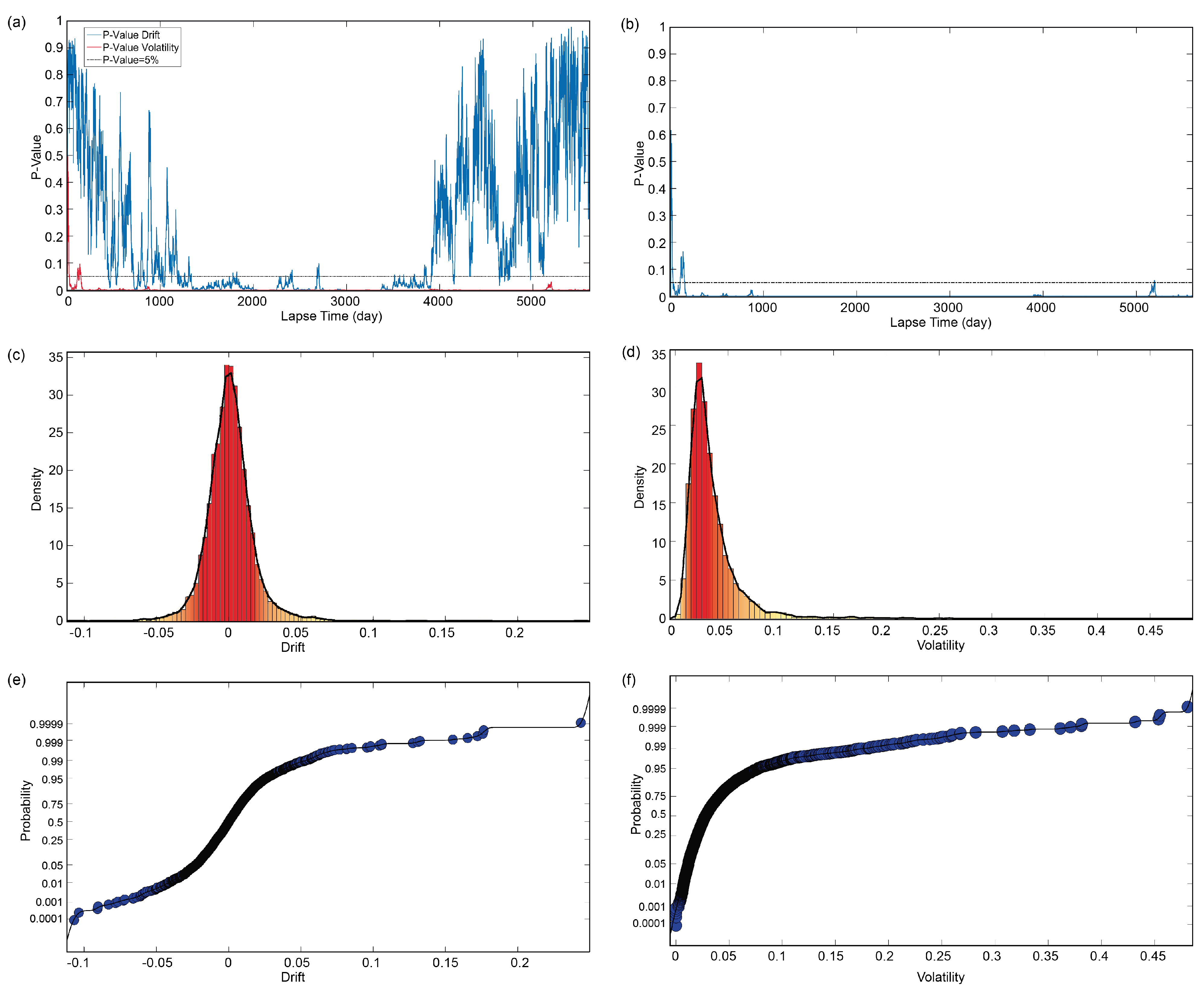
We show the evolution of the significance level with the time lapse for both volatility and drift in Figure 3a. In order to identify the best possible time lapse for both drift and volatility simultaneously, we calculate the F1 score of the significance level of both statistics according to Equation (44):
F 1 = 2 · α d r i f t · α v o l a t i l i t y α d r i f t + α v o l a t i l i t y .
The F1 score for maximum significance is reached for a time lapse of 7 days; see Figure 3b. The frequency histogram for both the gas price drift and volatility is calculated for this time lapse, and the corresponding adjustment is made using the KDE method; see Figure 3c,d. We show the significance values for the 7 days and the corresponding F1 scores in Table 2.
Additionally, we use a PDF adjusted with the KDE to calculate the initial price of each price trajectory in this scenario. This indicator is denoted as P ^ 0 .
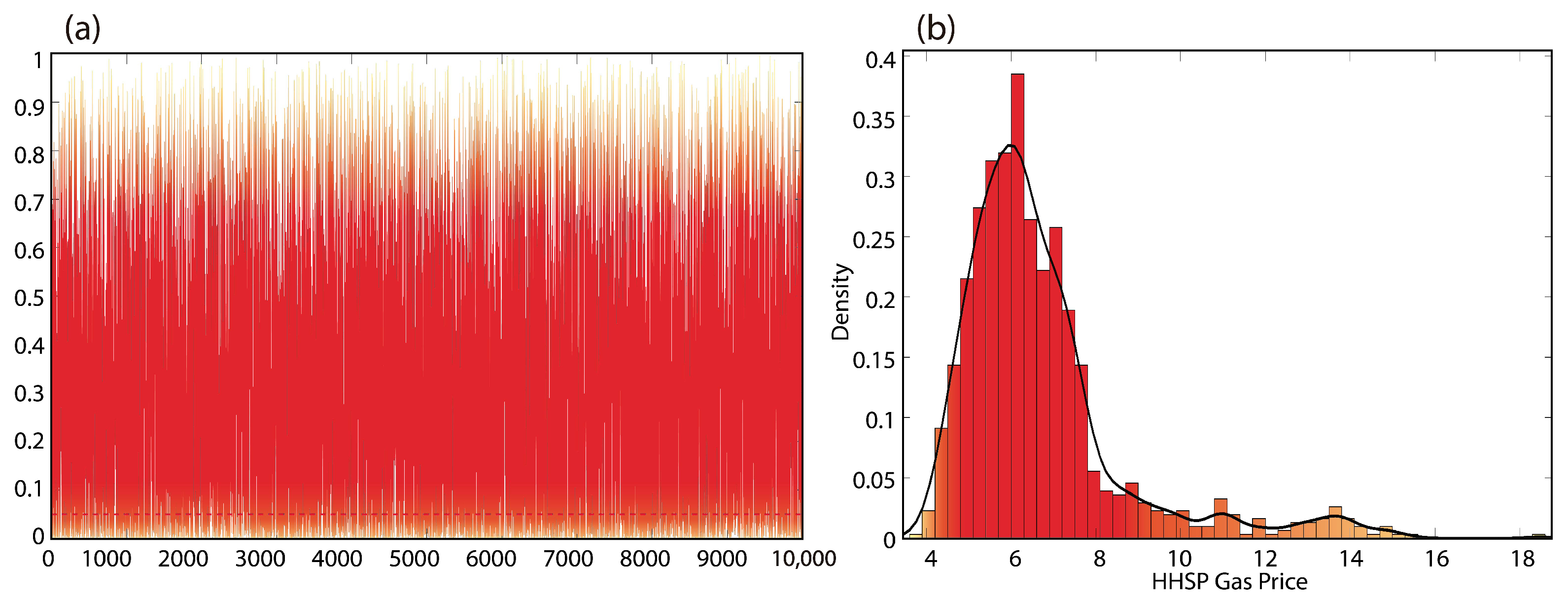
We determine the most suitable PDF by performing a random sweep of 10,000 realization time lapses and start dates across the entire “lapse vs. start date” space within the historical HHSP period. We omit a sweep of all the possible options since this would have an excessive computational cost and does not present substantial advantages compared to a sufficiently large random sampling. Analyzing all the options of the sample space would involve a study on the order of 5800 2 empirical functions of probability distribution, their corresponding adjustments of PDF non-parametric functions using KDE, and a K–S test to determine the level of significance of the adjustment. Instead of this, with the sampling of the 10,000 possible combinations taken at random, it is determined that, for a time lapse of 1021 days and the starting date of the period as 14 March 2001, a PDF non-parametric distribution can be fitted with a p-value of 0.9062; see Figure 4. This PDF is used to calculate the P ^ 0 at the start of each price trajectory.
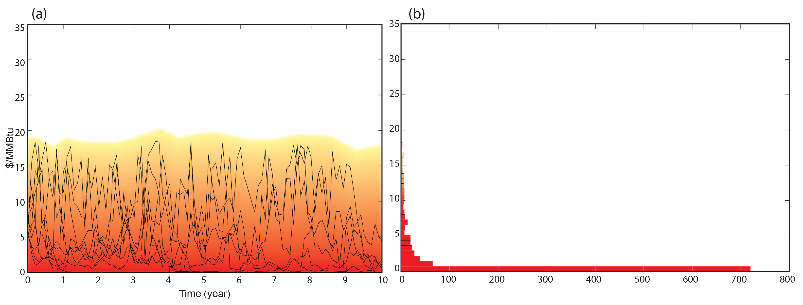
Finally, we apply the Monte Carlo method [84,85] by performing 1000 numerical simulations of the gas price trajectories using the GBM equations, considering a random initial price for each trajectory according to the calculated PDF distribution, and varying the drift and volatility at each time step of each gas price trajectory following the PDFs estimated. This generates a trajectory structure that closely resembles the historical gas price structure. Figure 5 displays 10 trajectories of the 1000 calculated, as well as the frequency distribution at the end of the 10-year period.

2.3. Statistical Calculation of Financial Indicators

In this study, we consider that CAPEX remains constant. We estimate that this hypothesis is reasonable since the number of fractures remains constant in the study (7 hydraulic fractures). In turn, each fractured ellipsoid maintains its volume constant, although its shape varies from more spherical to flatter. The volumes of the fractured ellipsoids are directly linked to the investment: volume of fluid injected and amount of proppants. If the ellipsoids are kept constant in volume, the investment in fracturing fluid and proppants is considered quasi-constant. The shape of the hydraulic fracture is associated with the greater skill of the operators in detecting the main direction of fracturing, which allows them to fire the initial projectiles in more or less accurate ways, but the perforating technique is not considered to significantly affect the CAPEX of the well.
In the next step of the methodology, we calculate the financial indicators Net Present Value (NPV), Internal Rate of Return (IRR), and Discounted Payback Period (DPP) statistically; that is, we calculate multiple values of each of them and again perform a non-parametric adjustment using Gaussian kernels (the KDE method).
The Net Present Value (NPV) is defined as the cash flow value for a determined investment, updated to the present moment in time. It is a dynamic indicator, as it considers the depreciation of monetary flows over time. N P V > 0 indicates a feasible investment, given that its value at the end of the operating lifespan will be positive. In general, the higher the NPV, the more attractive the investment. NPV = 0 indicates a financially neutral investment. N P V < 0 indicates an unprofitable investment that should not be undertaken.
The Internal Rate of Return (IRR) is defined as the discount rate value that gives an NPV of 0. It is the interest rate at which the cash flows equal the value of the investment made, and therefore the closest financial indicator to the commonly used concept of profitability of a financial product like an investment fund or government bond. An IRR that exceeds the expected for a financial product, considered risk-free, makes the investment appear attractive. Another way to analyze this indicator is to check if the IRR obtained in the investment analysis is greater than the expected depreciation or discount rate, in which case it can also be considered a viable investment. Both the NPV and IRR have been used in the study of shale-gas investments by authors such as [14,17,38,86,87,88,89,90,91,92].
The Break Even (BE) point, or profitability threshold, is the number of productive units after which studied investment enters into positive profitability [93]. In other words, Break Even can be considered as the time, expressed in units sold, at which the gains equal the fixed and variable costs of the investment. In this article, we propose a financial indicator based on the traditional idea of BE, which characterizes the time at which a shale-gas well achieves a positive valuation. The proposed indicator, termed Discounted Payback Period (DPP), is the time at which the NPV turns positive (the Break Even time). This indicator considers the dynamic evolution of gas price, the gas production according to physics, as well as the discounts and reductions in cash flows caused by inflation, operating costs, royalties and taxes. Figure 6 presents a graphical illustration of the idea behind the DPP.
Mathematically, the NPV, IRR, and DPP can be expressed as shown in Equations (45) to (47). This formula uses classical terminology in the O&G industry regarding asset evaluation:
N P V = i = 1 N ( 1 R a t e T ) · P g a s ( i ) · M s c f ( i ) · ( 1 R o y ) O P E X ( 1 + C P I d ( C P I g a s y ( i ) ) ) i C A P E X ,
0 = i = 1 N ( 1 R a t e T ) · P g a s ( i ) · M s c f ( i ) · ( 1 R o y ) O P E X ( 1 + I R R ) i C A P E X .
D P P = T i m e | N P V = 0
The terms appearing in Equations (45)–(47) are as follows:
  • CAPEX or Capital Expenditure is the financial value of the investment in the shale-gas well expressed in USD. We consider an investment of 4.8 million USD as the estimated cost of a shale-gas well of 1500 m length with 7 hydraulic fractures located at 3000 m depth.
  • i is the time step.
  • N represents the total time steps.
  • P g a s ( i ) is the gas price at the time step i, its value expressed in USD/Mscf.
  • M s c f ( i ) is the flow rate at time step i, its value expressed in Mscf/d. When this value is multiplied by P g a s ( i ) , the gross cash flows for time step i are obtained.
  • Roy refers to royalties, expressed on a unit basis, paid to the owner of the land and other agents such as county administrations in some cases. We assume a constant rate of 15% of the gross economic flow.
  • OPEX or Operational Expenditures are the well operating costs. We estimate a constant cost value of 150 USD/day. It is sometimes expressed in units of USD/Mscf, showing that its importance decreases as gas production drops. In this case, we consider it fixed and constant day to day. It is assumed as a hypothesis that day-to-day operations costs (OPEX) are constant since gas extraction management is carried out in an automated manner [14].
  • C P I d refers to daily inflation and depends on ( C P I g a s y ( i ) ) . That is, it depends on the annualized gas price inflation. This varies with each time step and is expressed on a unit basis. The annualized discount rate ranges from −0.1% to 1.75% over the life of the well.
  • RateT represents the profit taxes expressed on a unit basis. We apply 21% tax, which is the current gross rate for corporate tax in the USA.

2.4. Optimization of Financial Indicators

The search for optimal design variables is based on exploring the parametric spaces of porosity, permeability, and fracture aspect ratio. For each triplet of values, a percentile calculation of the NPV, IRR, and DPP indicators is performed, and the iso-probability curves are calculated, which determine the optimal parameter combinations.
The proposed modeling workflow can be described as follows:
An induced porosity–permeability field is defined in which parameter values vary between 1% and 5% for the porosity and between 1 and 10 μ d induced permeability in the SRV. There are 9 intervals of variation of porosity (0.5% increase per interval) and 11 intervals of variation of permeability (0.9 μ d of increase per interval). We generate 99 “porosity-induced permeability” pairs, calculating the corresponding production curve or flow-rate for each one.
Each production curve is combined with the 1000 price realizations. With the economic production curves ( M s c f × P r i c e g a s ), the statistical percentiles of the financial indicators are calculated (NPV, IRR, and DPP).
This same operation is performed for half-length ellipsoidal fractured volumes of 150 m, 200 m, and 250 m. The longer the axis, the flatter the ellipsoids. For certain financial indicators (NPV, IRR, or DPP) and risk level (X%), we determine the threshold value for which the investment is consider admissible. For NPV and IRR, we set the threshold at 0 USD/% or higher, and for DPP in 7 years or less.
Based on the porosity–permeability combinations, we perform a minimization of the absolute NPV and IRR percentiles adopted and a minimization of the absolute value of the DPP minus 7. Thus, if we decide to assume a risk of X0%, the absolute NPV, IRR, and DPP-7 values should be minimized, and the porosity–permeability combination that generates that minimum is a curve in the porosity–permeability plane for a PX0 percentile. This combination will also define a region in this plane in which the probability of achieving a positive NPV and IRR will be at least 100–X0%, or a region where the DPP will be less than 7 years with the same probability.
The steps summarized above can be expressed mathematically as:
m i n | N P V P X 0 ϕ , k , a | ,
ϕ ( 0 , 5 ) % , k ( 1 , 10 ) μ d , a = { 150 , 200 , 250 } m ,
m i n | I R R P X 0 ϕ , k , a | o r I R R P X 0 ϕ , k , a = 0 ,
ϕ ( 0 , 5 ) % , k ( 1 , 10 ) μ d , a = { 150 , 200 , 250 } m ,
m i n | D P P P X 0 ϕ , k , a 7 | o r D P P P X 0 ϕ , k , a = 7 ,
ϕ ( 0 , 5 ) % , k ( 1 , 10 ) μ d , a = { 150 , 200 , 250 } m .
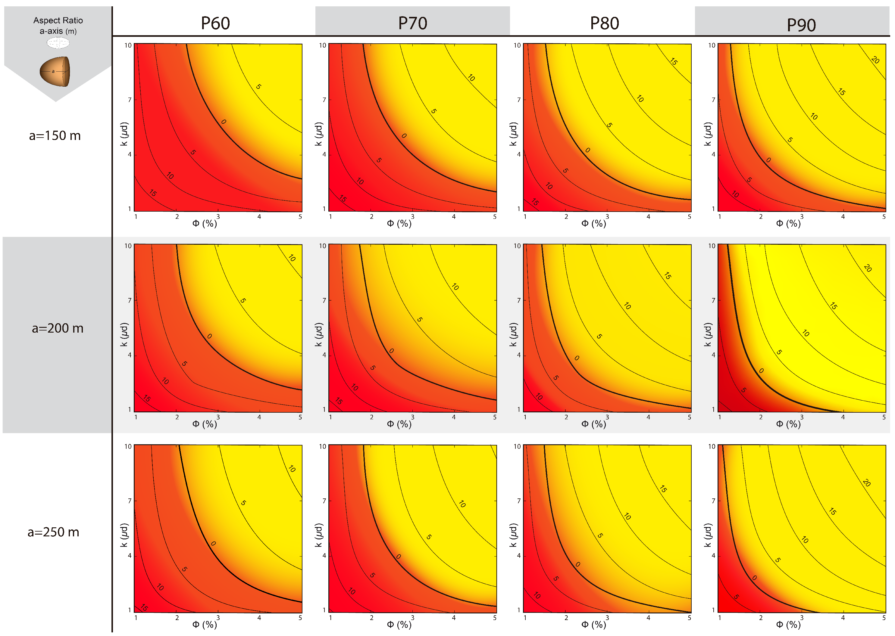
We analyze the P60–90 percentiles of NPV as a function of fracture geometry (Figure 7). The absence of parametric combinations that yield percentiles lower than 60% illustrates the complexity of getting a good location for a shale-gas well and an appropriate design; see Figure 7, Figure 8 and Figure 9. In Figure 7 and Figure 8, the region with the parameter combinations in yellow guarantees positive NPVs and IRRs with a probability 100–PX0%, while in the area of red colors, the parameter combinations indicate that the NPVs will be negative, with the probability PX0%. The thick black line marks the limit between negative and positive values of NPVs and shows the parametric combinations that minimize the objective function.
In practice, we resort to minimization of high percentile functions (60% and higher). This is because the shale-gas production process is very demanding in terms of petrophysical and design parameters (Figure 7 and Figure 8). Designs that allow a considerable increase in permeability and generate a fracture flatness that guarantees a high fracture surface and late time interference between fractures are needed to render the investment profitable.
The DPP financial indicator characterizes the moment that the NPV goes from negative to positive in a shale-gas investment. Taking into account that the expected life of a standard well is 10 years, we assume that the investment is attractive if the valuation of the shale-gas well becomes positive after 7 years. This would be 70% of the useful life of the investment. As in the case of IRR and NPV, the results from P60 to P90 are reflected in Figure 9. However, in this case, the interpretation of the graphs is slightly different: DPP decreases monotonically in all its percentiles with the improvement in the parameters. This renders large parametric values attractive, as in the case of NPV and IRR, but the probability of occurrence of some DPPs in the yellow areas (good parametric values) of Figure 9 is PX0%. In the red areas, the probability of occurrence is 100–X0%.

2.5. Aggregate Results of Financial Indicators

We summarize all the calculations performed to achieve optimized shale-gas well design. This aggregation appears in Figure 10, which can be considered as a scientific design guide for shale-gas wells. As an example of the usefulness of this aggregate calculation, design answers could be given in different circumstances. Suppose that an unconventional block in which the porosity is 5% is going to be exploited by the shale-gas well presented in this paper over the course of 10 years. Observing Figure 10, a design with 150 m of EPV half-axis and 7 μ d of induced permeability could be recommended to assure positive inversion with a 40% certainty. Another query could be that an O&G operator has a shale-type formation exploitation system that achieves a very flat fracturing geometry (250 m semi-ellipsoid axis), reaching an induced permeability of 8 μ d. In this situation, what field of porosities would a formation have to exploit with 60% security that allow us to recover the investment 7 years after starting the exploitation (or earlier)? The answer to this question would be, observing Figure 10, between 3.5% and 5% or, in any case, always higher than 3.5%.

3. Results and Discussion

After the calculations in the optimization process, which appear compacted and summarized in Figure 7, Figure 8, Figure 9 and Figure 10, we move on to analyze the results and discuss their meaning. As the statistical percentiles decrease from P90 to P60, the parametric region of positive NPV decreases. In turn, as the geometry of the fractured volumes becomes more spherical, this NPV-positive region is further reduced. This means that the lower the risk to be assumed and the less flat the fractured volumes are, higher the porosities and induced permeabilities will be required in order to guarantee a successful economic exploitation of the shale-gas well.
For a given percentile and semi-axis of the ellipsoid fractured volume, the locus of parametric combinations with NPV = 0 is a smooth curve on the porosity–permeability plane (Figure 7). Likewise, the curves of other NPV values, whether negative or positive, also present a smooth behavior, without breaks. The curves of the NPVs are shown equidistributed throughout the plane (Figure 7). Parametric regions and curves of the IRR have a behavior analogous to that of the NPV (Figure 8).
By comparing the regions of NPV positive and IRR positive for the same half-axis of the fractured volumes and for the same statistical percentile, we observe that IRR presents a greater surface area (Figure 7 and Figure 8). IRR is a less demanding financial indicator than the NPV. In any case, if the NPV shows a negative value for a certain parametric combination, the shale-gas investment must be discarded regardless of the IRR value. The parametric regions in DPP have a qualitative behavior very similar to that shown for NPV and IRR, but the curves that define these regions present quite a few breaks and instabilities (Figure 9). This is due to the difficulty of performing non-parametric PDF adjustments using the KDE method (see the significance level and bandwidth in Figure 6).
Regarding the parametric regions with a DPP less than 7 years (yellow region), we show how these have a quantitative behavior inverse to NPV and IRR. This is because the DPP curves are monotonically decreasing. As the percentile value increases and the flatness of the fractured volumes decreases, the DPP area less than 7 years (yellow region) disappears; see Figure 9.
Figure 10 presents the contours of different percentiles, with three ellipsoid fractured volume semi-axes, for NPV = 0 USD, IRR = 0%, and TBE = 7 years. These curves show a very similar behavior. They tend to cluster at low parametric values for both porosity and permeability (dark red zone) and tend to be further apart as we approach better parametric values (light yellow zone); see Figure 10. Note that the DPP P90 does not appear in the graphs for any value of the EPV semi-axis. This is because the parametric requirement is very high to ensure that 90% of the time a null value investment is achieved within 7 years (Figure 10).
By comparing the isocurves of DPP P80 and NPV P60, we observe that the parametric requirement to get the NPV to be 0 at 7 years or less after starting the investment with 80% security is not much higher than the parametric requirement to get the NPV to be 0 USD or greater than after 10 years of investment with 40% (100–60%) security. The petrophysical and design parameters necessary to achieve a positive investment value ( N P V > 0 ) are very demanding for an acceptable level of risk or acceptable probability of occurrence (yellow areas in Figure 7, Figure 8 and Figure 9).
Out of the three financial indicators we studied, the DPP is the one that requires the most favorable parameters to achieve a favorable investment evaluation; it is more demanding than the IRR and the DPP. There is no yellow area in DPP P90 (Figure 9).
Focusing on the NPV and IRR indicators, the most demanding one in terms of design parameters is the NPV. If an investment in shale-gas has a negative NPV and a positive IRR, this rules out the investment. From a decision-making point of view, NPV is the limiting indicator. Shale-gas production, understood as an investment, turns out to be a high-risk business, with a high probability of large profits, but also with a high probability of large losses (Figure 7).
The DPP optimization graphs (Figure 9) suggest that positive NPVs can be achieved relatively quickly for a given probability level and for a very wide parametric range. This supports the idea of treating the shale-gas production business as a speculative type business in which, once the risk of the initial investment has been eliminated, a rapid divestment and collection of capital gains is carried out via the sale of assets. This also eliminates the risk inherent to the evolution of production and especially of gas prices in the remaining three years of investment.

4. Conclusions

We have found that, for an investment in shale-gas to be profitable with high certainty, it is required that both the petrological parameters and the fracturing technology be extraordinarily good; simply having good parameters are not enough. Thus, if we use the NPV as a financial indicator for decision-making, we observe that, to achieve a positive investment after 10 years and with a statistical percentile of 60%, we will need, jointly: (i) a permeability in the stimulated domain of 4 to 10 μ D (three orders of magnitude more than the original rock matrix), (ii) a porosity of between 3.5% and 5%, and (iii) a practically flat fractured volume with a half-length of 250 m. If the IRR is adopted as a financial decision indicator, to achieve a positive return of 10% over the 10 years of the investment’s life, or the 60% percentile, the following are required: (i) an induced permeability in the stimulated zone of between 7 and 10  μ D, (ii) a porosity of between 4.5% and 5%, and (iii) a geometry of a flat fractured volume with a semi-length of 250 m. Finally, analyzing the recovery time of the investment, for the DPP to be less than 7 years with a percentile of 80% if the fracture is relatively spherical (semi-length of 150 m), porosity and induced permeability are required at the maximums of the ranges of this study, i.e., 5% and 10  μ D. The high level of parametric demand that a good investment in shale-gas implies supports the theory known as “sweet spots”. According to this theory, although shale-gas resources are very abundant in the world, with the current technology, only a few “sweet” areas meet the appropriate characteristics to be exploited profitably in terms of economics. These sweet areas are those that are being intensively exploited in the great basins of the USA, such as Marcellus, Barnet, Bakken, or Eagle Ford [94].
To precisely fine-tune the location of the shale-gas wells, a powerful campaign of petrological and geomechanical characterization of the blocks in which the shale-gas operations will be developed is required. This is the only way to reduce risk from the heterogeneity and uncertainty of shale-like exploration. In the event that the O&G operator discovers that he has been assigned a shale block with very poor petrology and with extremely low porosity, 1% can make the investment profitable. For this specific case, a positive NPV with a 90% percentile could be achieved with hydraulic stimulation that increases the permeability of the entire volume to 7  μ D or more, achieving high flatness of the fracturing volume (semi-axis 250 m). Our study shows that, with adequate fracturing technology, the operator can obtain enough gas to guarantee a sufficiently profitable investment even if the formation is naturally not ideal from a petrological point of view.
We have scientifically defined parametric maps that allow us to know the probability of achieving a certain value in a financial indicator. These design maps allow us to observe that achieving a profitable shale-gas well with guarantees is not impossible, but it is extraordinarily complex. The aggregated parametric mapping of NPV, IRR, and DPP that we have carried out sheds light on what parametric combination guarantees a positive investment or an early return on investment for a certain percentile. In this way, an NPV at least equal to zero with a percentile of 70% can be guaranteed with a combination of porosity, induced permeability, and EPV half-length that takes the values 3%, 7  μ D, and 150 m. Using the same parameter map, we can achieve a return on investment in seven years with a statistical percentile of 70%, with the semi-length of the ellipsoids being 200 m with the following parametric combinations: (5%, 2  μ D ), (2.5%, 4  μ D), or (1.5%, 10  μ D). As can be seen, the relationships between parameters are inverse and relatively easy to parameterize, which can be very useful in making financial decisions in shale-gas.
Shale-gas considered from the investment point of view is a high-risk business, which requires very good optimization of the block or formation in operation.
The NPV financial indicator is more demanding than the IRR. In fact, in some cases, there are discrepancies between the two. This result was not evident, but it positions NPV as the indicator with to make financial decisions in shale-gas wells. Comparison of NPV and IRR results with DPP results shows that investments in shale-gas are speculatively safer.
These conclusions lead us to the conviction that in shale-gas field there is still a long scientific and technological path. A route that makes it possible to make the most of these fossil resources in the most economically efficient way will undoubtedly have a very positive impact on companies (increased profits), consumers (reduced prices), and the environment (exploitation of an abundant and relatively clean resource).

Author Contributions

Conceptualization, A.S. and L.C.-F.; methodology, A.S.; software, L.C.-F.; validation, R.J., I.C. and L.C.-F.; formal analysis, L.C.-F.; investigation, A.S.; resources, L.C.-F.; data curation, A.S.; writing—original draft preparation, A.S.; writing—review and editing, R.J., I.C. and L.C.-F.; visualization, A.S.; supervision, I.C.; project administration, L.C.-F.; funding acquisition, I.C. All authors have read and agreed to the published version of the manuscript.

Funding

This research has been partially funded by the Ministry of Universities of the Spanish Government (grant: Subsidies to Public Universities for the Requalification of the Spanish University System, “Margarita Salas” Grants Modality for the Training of Young Doctors, RD 289/2021 of April 20), by strategic projects oriented towards the ecological transition and the digital transition of the Ministry of Science and Innovation: GREEN-HUGS (grant #TED2021-129991B-C31 and grant #TED2021-129991B-C32) and NEPTUNE (grant #TED2021-129805B-I00), by the Department of Education and University Planning of the Xunta de Galicia (grant #ED431C 2022/06), and by the Group of Numerical Methods in Engineering of the Universidade da Coruña.

Data Availability Statement

The data used in this article are, on the one hand, data on gas price quotes, and on the other, data related to numerical simulations. Gas price quote data can be found on the website of from the U.S. Energy Information Administration: https://www.eia.gov (Henry Hub Spot Price). On the other hand, the data related to the numerical simulations are included in the article itself.

Conflicts of Interest

The authors declare no conflicts of interest.

Abbreviations

The following abbreviations are used in this manuscript:
O&Goil and gas
Mscfthousand standard cubic feet
CAPEXCapital Expenditure
OPEXOperational Expenditures
NPVNet Present Value
IRRInternal Rate of Return
DPPDiscounted Payback Period

References

  1. Weber, C.L.; Clavin, C. Life cycle carbon footprint of shale gas: Review of evidence and implications. Environ. Sci. Technol. 2012, 46, 5688–5695. [Google Scholar] [CrossRef] [PubMed]
  2. Rivard, C.; Lavoie, D.; Lefebvre, R.; Séjourné, S.; Lamontagne, C.; Duchesne, M. An overview of Canadian shale gas production and environmental concerns. Int. J. Coal Geol. 2014, 126, 64–76. [Google Scholar] [CrossRef]
  3. Bowker, K.A. Barnett Shale gas production, Fort Worth Basin: Issues and discussion. AAPG Bull. 2014, 91, 523–533. [Google Scholar] [CrossRef]
  4. Chebeir, J.; Asala, H.; Manee, V.; Gupta, I.; Romagnoli, J.A. Data driven techno-economic framework for the development of shale gas resources. J. Nat. Gas Sci. Eng. 2019, 72, 103007. [Google Scholar] [CrossRef]
  5. Gao, J.; You, F. Game theory approach to optimal design of shale gas supply chains with consideration of economics and life cycle greenhouse gas emissions. AIChE J. 2019, 63, 2671–2693. [Google Scholar] [CrossRef]
  6. Rao, V. Shale Gas Drives Vertical Integration. J. Pet. Technol. 2014, 66, 18–19. [Google Scholar] [CrossRef]
  7. Hsu, C.S.; Robinson, P.R.; Hsu, C.S.; Robinson, P.R. Midstream transportation, storage, and processing. In Petroleum Science and Technology; Springer: Cham, Switzerland, 2019; pp. 385–394. [Google Scholar] [CrossRef]
  8. Quevedo-Orozco, D.R.; Ríos-Mercado, R.Z. Improving the quality of heuristic solutions for the capacitated vertex p-center problem through iterated greedy local search with variable neighborhood descent. Comput. Oper. Res. 2015, 62, 133–144. [Google Scholar] [CrossRef]
  9. Behrooz, H.A.; Boozarjomehry, R.B. Dynamic optimization of natural gas networks under customer demand uncertainties. Energy 2015, 134, 968–983. [Google Scholar] [CrossRef]
  10. Bellout, M.C.; Echeverría Ciaurri, D.; Durlofsky, L.J.; Foss, B.; Kleppe, J. Joint optimization of oil well placement and controls. Comput. Geosci. 2012, 16, 1061–1079. [Google Scholar] [CrossRef]
  11. Chang, C.; Liu, C.; Li, Y.; Li, X.; Yu, W.; Miao, J.; Sepehrnoori, K. A Novel Optimization Workflow Coupling Statistics-Based Methods to Determine Optimal Well Spacing and Economics in Shale Gas Reservoir with Complex Natural Fractures. Energies 2020, 13, 3965. [Google Scholar] [CrossRef]
  12. Gao, J.; You, F. Design and optimization of shale gas energy systems: Overview, research challenges, and future directions. Comput. Chem. Eng. 2017, 106, 699–718. [Google Scholar] [CrossRef]
  13. Guerra, O.J.; Calderon, A.J.; Papageorgiou, L.G.; Siirola, J.J.; Reklaitis, G.V. An optimization framework for the integration of water management and shale gas supply chain design. Comput. Chem. Eng. 2016, 92, 230–255. [Google Scholar] [CrossRef]
  14. Wilson, K.C.; Durlofsky, L.J. Optimization of shale gas field development using direct search tecniques and reduce-physics models. J. Pet. Sci. Eng. 2013, 108, 304–315. [Google Scholar] [CrossRef]
  15. Maxwell, S. Microseismic hydraulic fracture imaging: The path toward optimizing shale gas production. Lead. Edge 2011, 30, 340–346. [Google Scholar] [CrossRef]
  16. Yu, W.; Sepehrnoori, K. An Efficient Reservoir-Simulation Approach To Design and Optimize Unconventional Gas Production. J. Can. Pet. Technol. 2014, 53, 109–121. [Google Scholar] [CrossRef]
  17. Rahmanifard, H.; Plaksina, T. Application of fast analytical approach and AI optimization techniques to hydraulic fracture stage placement in shale gas reservoirs. J. Nat. Gas Sci. Eng. 2010, 52, 367–378. [Google Scholar] [CrossRef]
  18. Onwunalu, J.E.; Durlofsky, L.J. Application of a particle swarm optimization algorithm for determining optimum well location and type. Comput. Geosci. 2010, 14, 183–198. [Google Scholar] [CrossRef]
  19. Yuan, J.; Luo, D.; Feng, L. A review of the technical and economic evaluation techniques for shale gas development. Appl. Energy 2015, 148, 49–65. [Google Scholar] [CrossRef]
  20. Li, C.; Eason, J.P.; Drouven, M.G.; Grossmann, I.E. Shale gas pad development planning under price uncertainty. AIChE J. 2020, 66, e16933. [Google Scholar] [CrossRef]
  21. Tang, S.L.; John Tang, H. The variable financial indicator IRR and the constant economic indicator NPV. Eng. Econ. 2003, 48, 69–78. [Google Scholar] [CrossRef]
  22. Guanche, R.; De Andres, A.D.; Simal, P.D.; Vidal, C.; Losada, I.J. Uncertainty analysis of wave energy farms financial indicators. Renew. Energy 2014, 68, 570–580. [Google Scholar] [CrossRef]
  23. Zhang, K. Comparative Analysis of NPV and IRR Indicators Based on Practical Applications. Highlights Bus. Econ. Manag. 2023, 7, 22–28. [Google Scholar] [CrossRef]
  24. Rushinck, A. Capital Budgeting Techniques, the Payback Period, the Net Present Value, the Internal Rate of Return and Their Computer Applications. Manag. Financ. 1983, 9, 11–13. [Google Scholar] [CrossRef]
  25. Bhandari, S.B. Discounted payback period-some extensions. J. Bus. Behav. Sci. 2009, 21, 28–38. [Google Scholar]
  26. Gorshkov, A.S.; Vatin, N.I.; Rymkevich, P.P.; Kydrevich, O.O. Payback period of investments in energy saving. Mag. Civ. Eng. 2018, 2, 65–75. [Google Scholar]
  27. Mohn, K.; Misund, B. Investment and uncertainty in the international oil and gas industry. Energy Econ. 2009, 31, 240–248. [Google Scholar] [CrossRef]
  28. Brockway, P.E.; Owen, A.; Brand-Correa, L.I.; Hardt, L. Estimation of global final-stage energy-return- on-investment for fossil fuels with comparison to renewable energy sources. Nat. Energy 2019, 4, 616–621. [Google Scholar] [CrossRef]
  29. Shirangi, M.G.; Durlofsky, L.J. A general method to select representative models for decision making and optimization under uncertainty. Comput. Geosci. 2016, 96, 109–123. [Google Scholar] [CrossRef]
  30. Ramos, S.B.; Veiga, H. Risk factors in oil and gas industry returns: International evidence. Energy Econ. 2011, 33, 525–542. [Google Scholar] [CrossRef]
  31. Domnikov, A.; Khomenko, P.; Chebotareva, G.; Khodorovsky, M. Risk and Profitability Optimization of Investments in the Oil and Gas Industry. Energy 2017, 2, 263–276. [Google Scholar] [CrossRef]
  32. Isebor, O.J.; Durlofsky, L.J. Biobjective optimization for general oil field development. J. Pet. Sci. Eng. 2017, 119, 123–138. [Google Scholar] [CrossRef]
  33. Yuhua, Z.; Dongkun, L. Investment optimization in oil and gas plays. Pet. Explor. Dev. 2009, 36, 535–540. [Google Scholar] [CrossRef]
  34. Tan, S.H.; Barton, P.I. Optimal shale oil and gas investments in the United States. Energy 2017, 141, 398–422. [Google Scholar] [CrossRef]
  35. Shirangi, M.G.; Durlofsky, L.J. Closed-loop field development under uncertainty by use of optimization with sample validation. SPE J. 2017, 20, 908–922. [Google Scholar] [CrossRef]
  36. Boulis, A.; Jayakumar, R.; Rai, R. A New Approach for Well Spacing Optimisation and Its Application to Various Shale Gas Resources. In Proceedings of the International Petroleum Technology Conference, Beijing, China, 26–28 March 2013. [Google Scholar] [CrossRef]
  37. Valle-Falcones, L.M.; Grima-Olmedo, C.; Rodríguez-Pons Esparver, R.; Zamarro-Toves, E. Evaluation and Economics of Shale Gas Reserves in the Flysch-Eocene Formation of the Jaca Basin. Appl. Sci. 2023, 13, 1732. [Google Scholar] [CrossRef]
  38. Weijermars, R. Economic appraisal of shale gas plays in Continental Europe. Appl. Energy 2013, 106, 100–115. [Google Scholar] [CrossRef]
  39. Soage, A.; Juanes, R.; Colominas, I.; Cueto-Felgueroso, L. The Impact of the Geometry of the Effective Propped Volume on the Economic Performance of Shale Gas Well Production. Energies 2021, 14, 2475. [Google Scholar] [CrossRef]
  40. Soage, M.A. A Numerical Modelling Framework for the Optimization and Economic Analysis of Unconventional Gas Production. Doctoral Thesis, University of A Coruna, A Coruña, Spain, 2021. [Google Scholar]
  41. Silin, D.; Kneafsey, T. Shale Gas: Nanometer-Scale Observations and Well Modelling. J. Canadian Petro. Tech. 2012, 464–475. [Google Scholar] [CrossRef]
  42. Cipolla, C.L.; Lolon, E.P.; Erdle, J.C. Rubin, B. Reservoir Modeling in Shale-Gas Reservoirs. SPE Reserv. Eval. Eng. 2010, 13, 464–475. [Google Scholar] [CrossRef]
  43. Patzek, T.W.; Male, F.; Marder, M. Gas production in the Barnett Shale obeys a simple scaling theory. Proc. Natl. Acad. Sci. USA 2013, 110, 304–315. [Google Scholar] [CrossRef]
  44. Wang, X.; Sheng, J. Gas sorption and non-Darcy flow in shale reservoirs. Pet. Sci. 2017, 14, 746–754. [Google Scholar] [CrossRef]
  45. Haider, S.; Saputra, W.; Patzek, T. The Key Factors That Determine the Economically Viable, Horizontal Hydrofractured Gas Wells in Mudrocks. Energies 2020, 13, 2348. [Google Scholar] [CrossRef]
  46. Starovoitova, B.N.; Golovin, S.V.; G.V. Paderin, G.V.; Shel, E.V.; Kavunnikova, E.A.; Krivtsov, A.M. Design optimization of hydraulic fracturing. IOP Conf. Ser. Earth Environ. Sci. 2018, 193, 0120115. [Google Scholar] [CrossRef]
  47. Yan, X.; Sun, H.; Huang, Z.; Liu, L.; Wang, P.; Zhang, Q.; Yao, J. Hierarchical modeling of hydromechanical coupling in fractured shale gas reservoirs with multiple porosity scales. Energy Fuels 2021, 35, 5758–5776. [Google Scholar] [CrossRef]
  48. Vandenbroucke, M.; Largeau, C. Kerogen origin, evolution and structure. Org. Geochem. 2007, 38, 719–833. [Google Scholar] [CrossRef]
  49. Cheng, Y.; Jiang, S.; Zhang, D.; Liu, C. An adsorbed gas estimation model for shale gas reservoirs via statistical learning. Appl. Energy 2017, 197, 327–341. [Google Scholar] [CrossRef]
  50. Tan, L.; Zuo, L.; Wang, B. Methods of Decline Curve Analysis for Shale Gas Reservoirs. Energies 2018, 11, 552. [Google Scholar] [CrossRef]
  51. Arias Ortiz, D.A.; Klimkowski, L.; Finkbeiner, T.; Patzek, T.W. The Effect of Hydraulic Fracture Geometry on Well Productivity in Shale Oil Plays with High Pore Pressure. Energies 2021, 14, 7727. [Google Scholar] [CrossRef]
  52. Yu, W.; Sepehrnoori, K.; Patzek, T.W. Evaluation of gas adsorption in Marcellus Shale. In Proceedings of the Annual Technical Conference and Exhibition, Amsterdam, The Netherlands, 27–29 October 2014. [Google Scholar] [CrossRef]
  53. Efron, B. The 1977 RIETZ lecture. Ann. Stat. 1979, 7, 1–26. [Google Scholar] [CrossRef]
  54. Clark, P.K. A Subordinated Stochastic Process Model with Finite Variance for Speculative Prices. Econom. J. Econom. Soc. 1973, 41, 135–155. [Google Scholar] [CrossRef]
  55. Metropolis, N.; Ulam, S. The Monte Carlo Method. J. Am. Stat. Assoc. 1949, 44, 335–341. [Google Scholar] [CrossRef] [PubMed]
  56. Zambom, A.Z.; Ronaldo, D. A review of kernel density estimation with applications to econometrics. Int. Econom. Rev. 2013, 5, 20–42. [Google Scholar]
  57. Wang, H.; Ma, F.; Tong, X.; Liu, Z.; Zhang, X.; Wu, Z.; Li, D.; Wang, B.; Xie, Y.; Yang, L. Assessment of global unconventional oil and gas resources. Pet. Explor. Dev. 2016, 43, 925–940. [Google Scholar] [CrossRef]
  58. McGlade, C.; Speirs, J.; Sorrell, S. Unconventional gas–a review of regional and global resource estimates. Energy 2013, 55, 571–584. [Google Scholar] [CrossRef]
  59. Dong, Z.; Holditch, S.A.A.; McVay, D.A.A.; Ayers, W.B.B. Global Unconventional Gas Resource Assessment. SPE Econ. Manag. 2012, 4, 222–234. [Google Scholar] [CrossRef]
  60. Pejman, T.; Javadpour, F.; Sahimi, M. Data mining and machine learning for identifying sweet spots in shale reservoirs. Expert Syst. Appl. 2017, E88, 435–447. [Google Scholar] [CrossRef]
  61. Qian, K.-R.; He, Z.-L.; Liu, X.-W.; Chen, Y.-Q. Intelligent prediction and integral analysis of shale oil and gas sweet spots. Pet. Sci. 2018, 15, 744–755. [Google Scholar] [CrossRef]
  62. Montgomery, J.B.; O’sullivan, F.M. Spatial variability of tight oil well productivity and the impact of technology. Appl. Energy 2018, 195, 344–355. [Google Scholar] [CrossRef]
  63. COMSOL Multiphysics. Introduction to COMSOL Multiphysics (2018); COMSOL Multiphysics: Burlington, MA, USA, 2018. [Google Scholar]
  64. Sakhaee-Pour, A.; Bryant, S.L. Gas permeability of shale. SPE Reserv. Eval. Eng. 2012, 15, 401–409. [Google Scholar] [CrossRef]
  65. Cui, G.; Liu, J.; Wei, M.; Feng, X.; Elsworth, D. Evolution of permeability during the process of shale gas extraction. J. Nat. Gas Sci. Eng. 2018, 49, 94–109. [Google Scholar] [CrossRef]
  66. Gao, Q.; Han, S.; Cheng, Y.; Li, Y.; Yan, C.; Han, Z. Apparent permeability model for gas transport through micropores and microfractures in shale reservoirs. Fuel 2021, 285, 119086. [Google Scholar] [CrossRef]
  67. Marder, M.; Chen, C.H.; Patzek, T. Simple models of the hydrofracture process. Phys. Rev. E 2015, 92, 062408. [Google Scholar] [CrossRef] [PubMed]
  68. Kwok, Y.K. Introduction to Derivative Instruments. In Mathematical Models of Financial Derivatives; Springer Finance: Berlin/Heidelberg, Germany, 2008. [Google Scholar] [CrossRef]
  69. Van Kampen, N.G. Stochastic differential equations. Phys. Rep. 1976, 24, 171–228. [Google Scholar] [CrossRef]
  70. Postali, F.A.; Picchetti, P. Geometric Brownian motion and structural breaks in oil prices: A quantitative analysis. Energy Econ. 2006, 28, 506–522. [Google Scholar] [CrossRef]
  71. Itô, K. On a formula concerning stochastic differentials. Nagoya Math. J. 1951, 3, 55–65. [Google Scholar] [CrossRef]
  72. Shiga, T.; Shimizu, A. Infinite dimensional stochastic differential equations and their applications. J. Math. Kyoto Univ. 1980, 20, 395–416. [Google Scholar] [CrossRef]
  73. Burrage, K.; Burrage, P.M.; Tian, T. Numerical methods for strong solutions of stochastic differential equations: An overview. Proc. R. Soc. Lond. Ser. A Math. Phys. Eng. Sci. 2004, 460, 373–402. [Google Scholar] [CrossRef]
  74. Doob, J.L. The Brownian movement and stochastic equations. Ann. Math. 1942, 43, 351–369. [Google Scholar] [CrossRef]
  75. Naseer, M.; Bin Tariq, D.Y. The efficient market hypothesis: A critical review of the literature. Iup J. Financ. Risk Manag. 2015, 12, 48–63. [Google Scholar]
  76. Ricciardi, L.M. On the transformation of diffusion processes into the Wiener process. J. Math. Anal. Appl. 1976, 54, 185–199. [Google Scholar] [CrossRef]
  77. Lepskii, O.V. On a problem of adaptive estimation in Gaussian white noise. Theory Probab. Its Appl. 1991, 35, 454–466. [Google Scholar] [CrossRef]
  78. Itô, K. 109.Stochastic Integral. Proc. Imp. Acad. 1944, 20, 519–524. [Google Scholar] [CrossRef]
  79. Parzen, E. On estimation of a probability density function and mode. Ann. Math. Stat. 1962, 33, 1065–1076. [Google Scholar] [CrossRef]
  80. Li, J.; Wu, Q.; Tian, Y.; Fan, L. Monthly Henry Hub natural gas spot prices forecasting using variational mode decomposition and deep belief network. Energy 2021, 227, 120478. [Google Scholar] [CrossRef]
  81. Lidén, J. Stock Price Predictions Using a Geometric Brownian Motion. Master’s Thesis, Uppsala University, Uppsala, Sweden, 2018. [Google Scholar]
  82. Massey, F.J. The Kolmogorov-Smirnov Test for Goodness of Fit. J. Am. Stat. Assoc. 1951, 46, 68–78. [Google Scholar] [CrossRef]
  83. Wand, M.P.; Schucany, W.R. Gaussian-Based Kernels. Can. J. Stat. 1990, 18, 197–204. [Google Scholar] [CrossRef]
  84. Papadopoulos, C.E.; Yeung, H. Uncertainty estimation and Monte Carlo simulation method. Flow Meas. Instrum. 2001, 12, 291–298. [Google Scholar] [CrossRef]
  85. Hacura, A.; Jadamus-Hacura, M.; Kocot, A. Risk analysis in investment appraisal based on the Monte Carlo simulation technique. Eur. Phys. J. B 2001, 20, 551–553. [Google Scholar] [CrossRef]
  86. Bas, E. A robust approach to the decision rules of NPV and IRR for simple projects. Appl. Math. Comput. 2013, 219, 5901–5908. [Google Scholar] [CrossRef]
  87. Lake, L.W.; Baylor, J.M.; Ramsey, J.D.; Titman, S. A Primer on the Economics of Shale Gas Production Just How Cheap is Shale Gas? J. Appl. Corp. Financ. 2013, 25, 87–96. [Google Scholar] [CrossRef]
  88. Yu, W.; Sepehrnoori, K. Optimization of Multiple Hydraulically Fractured Horizontal Wells in Unconventional Gas Reservoirs. J. Pet. Eng. 2013, 2013, 151898. [Google Scholar]
  89. Eshkalak, M.O.; Aybar, U.; Sepehrnoori, K. An Economic Evaluation on the Re-fracturing Treatment of US Shale Gas Resources. In Proceedings of the Eastern Regional Meeting, Charleston, WV, USA, 21–23 October 2014. SPE 171009-MS. [Google Scholar]
  90. Du, Y.; Liu, H.; Sun, Y.; Sheng, S.; Wei, M. An Improved Integrated Numerical Simulation Method to Study Main Controlling Factors of EUR and Optimization of Development Strategy. Energies 2023, 16, 2011. [Google Scholar] [CrossRef]
  91. Nguyen-Le, V.; Shin, H. Development of Reservoir Economic Indicator for Barnett Shale Gas Potential Evaluation Based on the Reservoir and Hydraulic Fracturing Parameters. J. Nat. Gas Sci. Eng. 2019, 66, 159–167. [Google Scholar] [CrossRef]
  92. Hong, B.; Li, X.; Song, S.; Chen, S.; Zhao, C.; Gong, J. Optimal planning and modular infrastructure dynamic allocation for shale gas production. Appl. Energy 2020, 261, 114439. [Google Scholar] [CrossRef]
  93. Kampf, R.; Majerčák, P.; Švagr, P. Break-Even Point Analyze. NašE More Znan. čAsopis More Pomor. 2016, 63, 126–128. [Google Scholar] [CrossRef]
  94. Lee, D.S.; Herman, J.D.; Elsworth, D.; Kim, H.T.; Lee, H.S. A Critical Evaluation of Unconventional Gas Recovery from Marcellus Shale, Northeastern United States. KSCE J. Civ. Eng. 2018, 15, 679–687. [Google Scholar] [CrossRef]
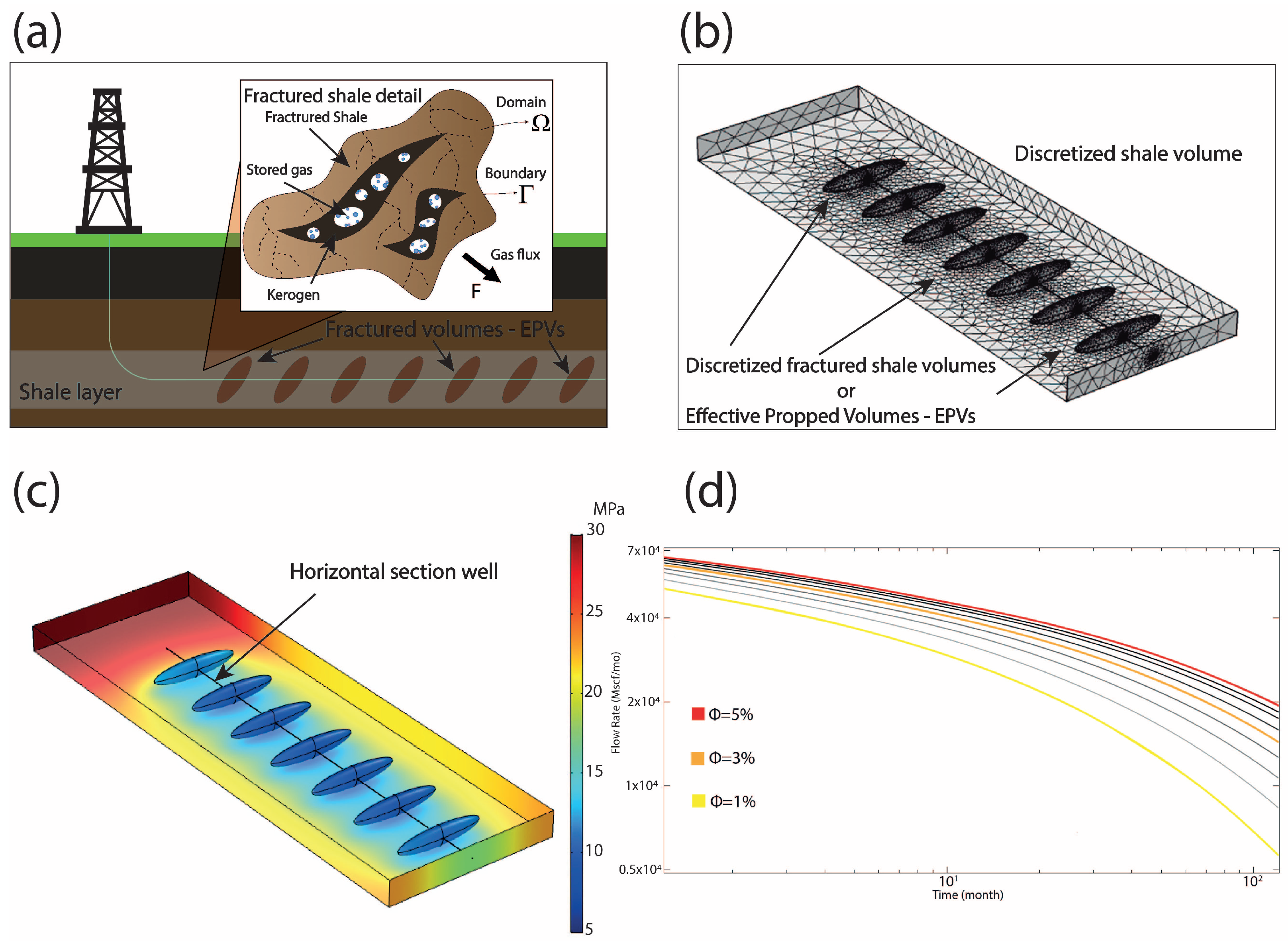
Figure 1. In this figure, we represent the process of numerical calculation of gas production in the standard well presented in this article. (a) Graphic representation of the standard shale-gas well. An inset shows the fractured shale formation; mathematically, this body is a control volume with a certain Ω domain and a Γ contour. Within the control volume, pores (holes), kerogen (dark brown), and methane are represented in the form of blue bubbles. (b) 3D numerical model of the shale-gas well. (c) Graphic representation of the pressure field 10 years after beginning methane extraction. The pressure scale has MPa units. (d) Methane production curves over time for different porosity values from 1% to 5%. Each curve represents a 0.5% increase in porosity compared to the previous curve. The curves with more intense gray have porosities closer to 5% and the lighter ones to 1%. We also indicate with warm colors the three most characteristic curves of the study (1%, 3% and 5%). The graphic representation is done on a decimal–logarithmic scale.
Energies 17 00864 g001
Figure 2. Top: general diagram of the bootstrapping method. Bottom: bootstrapping applied to the gas price series.
Energies 17 00864 g002
Figure 3. (a) Significance level of drift and volatility for each time lapse expressed on a unit basis. The significance level limit of 0.05 or 5% is indicated by a dashed black line. (b) F1 scores combine significance levels for drift and volatility. The limit is indicated by a dashed black line. (c) Drift frequency and KDE adjustment of the PDF for a 7-day time lapse. (d) Volatility frequency and KDE adjustment of the PDF for a 7-day time lapse. (e) Comparison between the inverse CDF of the drift calculated using the non-parametric function with the KDE method (black curve) and the empirical data (blue dots). (f) Comparison between the inverse CDF of the drift calculated using the non-parametric function with the KDE method (black curve) and the empirical data (blue dots).
Energies 17 00864 g003
Figure 4. (a) Statistical significance level of the 10,000 random samples. (b) Empirical distribution and adjustment of PDF by the nonparametric KDE method of the initial price, P ^ 0 . Lapse time = 1021 days, and start date is 3 March 2001. Dark reds indicate high concentrations of realizations or frequency, and bright yellow colors indicate low concentrations of realizations or frequencies.
Energies 17 00864 g004
Figure 5. (a) Examples of realizations and price density maps for 1000 realizations of price evolution. Only 10 of the 1000 simulations carried out are shown. The outputs with the maximum value, minimum value, and 8 random intermediate values are shown. We indicate on a warm color scale graph the concentration of trajectories; the area with higher concentration of price trajectories is in dark red, and the area containing the lower concentration is in bright yellow. (b) Histogram of price frequencies at the end of the 10-year period.
Energies 17 00864 g005
Figure 6. (a) Graphical representation of the DPP calculation (b) Results of the DPP (years) analysis presented in matrix form. The vertical axis represents the variations of the gas production parameters (petrological and design). The horizontal axis represents the different price scenarios S1 to S4. The percentages P10, P50, and P90 are represented for each result, and the areas with a higher concentration (red) and lower concentration (yellow) of realizations are shown using a warm color scale. The area with the higher concentration corresponds with the distribution mode of the adjusted PDF function. For each result, a graph is inserted showing the statistical significance level of the adjustment of the nonparametric function (blue dots) on a scale of 0 to 1. We use red dots in the insets to indicate the normalized bandwidth by 10-year value of the Gaussian kernels that were used to adjust the PDF.
Energies 17 00864 g006
Figure 7. NPV values expressed in USD for each statistical percentile indicated. The NPVs are calculated for each value of the semi-axis a of the EPVs, and we set the parameters for each pair as induced permeability (vertical axis and μ d scale) and porosity (horizontal axis and scale in %). We show different NPV isoline values drawn in a thin black line. A thick black line defines the parametric combination of NPV = 0 or optimization of Equation (48). The yellow areas indicate parametric combinations that generate a positive NPV, and the red areas indicate parametric combinations that generate a negative NPV.
Energies 17 00864 g007
Figure 8. IRR values expressed in % for each statistical percentile indicated. The NPVs are calculated for each value of the semi-axis a of the EPVs, and we set the parameters for each pair as induced permeability (vertical axis and μ d scale) and porosity (horizontal axis and scale in %). We show different NPV isoline values drawn in a thin black line. A thick black line defines the parametric combination of IRR = 0 or optimization of Equation (48). The yellow areas indicate parametric combinations that generate a positive IRR, and the red areas indicate parametric combinations that generate a negative IRR.
Energies 17 00864 g008
Figure 9. DPP values expressed in years for each statistical percentile indicated. The DPPs are calculated for each value of the semi-axis a of the EPVs, and we set these parameters for each pair as induced permeability (vertical axis and μ d scale) and porosity (horizontal axis and scale in %). We show different DPP isoline values drawn in a thin black line. A thick black line defines the parametric combination of DPP = 7 or optimization of Equation (52). The yellow areas indicate parametric combinations that generate a DPP less than 7 years, and the red areas indicate parametric combinations that generate a DPP greater than 7 years.
Energies 17 00864 g009
Figure 10. Aggregate graphical representation of the percentiles of NPV = 0 USD, IRR = 0 %, and DPP = 7 years over the fields (k, ϕ ) and for each semi-axis value a perpendicular to the well.
Energies 17 00864 g010
Table 1. Variables and parameters.
VariableMeaningValue
P x , t gas pressure[30–35 MPa]
P r initial reservoir pressure30 MPa
P b h p bottom hole pressure5 MPa
c g gas compressibility 3.979 × 10 6 [ s 2 / m 2 ]
c f Langmuir isotherm slope  -
ϕ porosity1–5%
ρ 0 methane density at standard conditions 0.717 [ k g / m 3 ]
ρ k kerogen density 1250 [ k g / m 3 ]
S k kerogen relative volume 10 %
V a Langmuir isotherm  -
V L Langmuir volume 0.00264 [ m 3 / k g ]
P L Langmuir pressure3 MPa
kfractured shale permeability 10 18 [ m 2 ] 10 17 [ m 2 ] 1 [ μ D ] 10 [ μ D ]
k E P V EPV permeability 2 × 10 15 [ m 2 ] 2 [ m D ]
μ methane viscosity 10 4 [ P a · s ]
qmethane fluxMscf/month ( 1 m 3 0.0353 M s c f )
Ω stimulated volume  -
n ¯ normal vector to contour Γ   -
Table 2. Drift and volatility values for S4.
p-Value–Time Lapse = 7 DaysF1 Score–Time Lapse = 7 Days
μ ^ 0.81270.6161
σ ^ 0.49610.6161
Disclaimer/Publisher’s Note: The statements, opinions and data contained in all publications are solely those of the individual author(s) and contributor(s) and not of MDPI and/or the editor(s). MDPI and/or the editor(s) disclaim responsibility for any injury to people or property resulting from any ideas, methods, instructions or products referred to in the content.