Abstract
Renewable energy production is one of the most important strategies to reduce the emission of greenhouse gases. However, wind and solar energy especially depend on time-varying properties of the environment, such as weather. Hence, for the control and stabilization of electricity grids, the accurate forecasting of energy production from renewable energy sources is essential. This study provides an empirical comparison of the forecasting accuracy of electricity generation from renewable energy sources by different deep learning methods, including five different Transformer-based forecasting models based on weather data. The models are compared with the long short-term memory (LSTM) and Autoregressive Integrated Moving Average (ARIMA) models as a baseline. The accuracy of these models is evaluated across diverse forecast periods, and the impact of utilizing selected weather data versus all available data on predictive performance is investigated. Distinct performance patterns emerge among the Transformer-based models, with Autoformer and FEDformer exhibiting suboptimal results for this task, especially when utilizing a comprehensive set of weather parameters. In contrast, the Informer model demonstrates superior predictive capabilities for onshore wind power and photovoltaic (PV) power production. The Informer model consistently performs well in predicting both onshore wind and PV energy. Notably, the LSTM model outperforms all other models across various categories. This research emphasizes the significance of selectively using weather parameters for improved performance compared to employing all parameters and a time reference. We show that the suitability and performance of a prediction model can vary significantly, depending on the specific forecasting task and the data that are provided to the model.
Keywords:
forecasting; solar energy; onshore wind; weather parameter; deep learning; Transformer; LSTM 1. Introduction
Humanity faces numerous challenges in the 21st century, with some of the most pressing issues being highlighted in the Global Risk Report 2022 by the World Economic Forum. One of the critical concerns addressed in this report is the escalating threat of climate change [1]. The main cause of climate change is the greenhouse effect caused by humans. The anthropogenic greenhouse effect amplifies the natural greenhouse effect, which is essential for life. This anthropogenic amplification has a significant influence on global warming [2]. The greenhouse effect is a process in which certain gases or greenhouse gases enable short-wave solar radiation to pass through Earth’s atmosphere. However, these greenhouse gases prevent the re-radiation of heat. Carbon dioxide is one of the greenhouse gases that is mainly responsible for energy-related emissions. Energy-related emissions arise from the generation of heat and electricity from fossil fuels. The energy industry is the main source of energy-related greenhouse gases. In 2020, energy-related emissions accounted for approx. 83% of German greenhouse gas emissions, with the energy industry accounting for 35% [3]. This is why it is important to generate electricity in as climate-neutral a way as possible. In this respect, it is crucial not to overlook the economic, social and ecological aspects and the associated possible consequences. These are the three pillars of the sustainability triangle. Additionally, the impact on the industry should be considered. Germany has chosen wind energy and photovoltaics as the cornerstone of its future energy supply in pursuit of its goal to become climate-neutral by 2045. Compared to brown coal ( emission factor of approx. 1080 g/kWh), a PV system has a emission factor of approx. 56 g/kWh. The emission factor can vary depending on the PV module, the country of production and its associated transport routes, and the share of renewable energy in the electricity mix of the country in which the PV modules are produced [4]. Onshore wind power plants have an even lower emission factor of 10.5 g/kWh [5]. However, this strategy brings with it many challenges. One of them is that renewable energies are highly dependent on the weather, so reliability is an important factor that must be considered. The risk of a power shortage increases with the possible occurrence of wind lulls and days with little sunshine. For this reason, the prediction of electricity generation by renewable energies is considered based on deep learning. The importance of accurate prediction is further underscored by the fact that these renewable energies have so far had to be supplemented by controllable power plants to ensure energy security.
Furthermore, we are facing ever more advanced digital transformation. Artificial Intelligence is one of the key technologies for digital progress and change. With the improvement of hardware performance, the development of new algorithms and an ever-increasing collection of datasets, we have been experiencing an AI boom for several years. This influences many areas of the economy up to and including the energy sector. The integration of AI into the energy sector has been transformative, revolutionizing the way we generate, distribute and consume energy. The use of AI has enabled unprecedented advancements in energy efficiency, grid management, renewable energy integration and demand response systems [6,7]. As we continue to embrace this digital transformation, AI’s role in the energy sector will only grow more prominent.
In light of the increasing focus on sustainability and energy independence, the integration of renewable energy sources like solar and wind AI has become more prevalent. Traditional power grids were primarily designed for energy generation from conventional energy sources. The growing incorporation of renewable energies necessitates a substantial revamp of existing grids. Renewable energies are variable and weather-dependent, meaning that power generation can fluctuate. This requires flexible grids capable of compensating for these fluctuations and efficiently distributing the generated energy. To manage this variability and ensure stability, accurate predictions of renewable energy production are essential for effective grid management and distribution [8,9]. For some years now, there has been a steady increase in publications in the field of PV and wind forecasting [10]. AI algorithms can analyze the impact of weather parameters, weather patterns, historical data and energy consumption trends to optimize the utilization of renewable resources. This allows for better forecasting of energy generation and helps in managing the intermittency associated with renewable sources, ensuring a more stable and reliable energy supply. There is a wealth of literature comparing different models in various renewable energy prediction scenarios, such as the prediction of wind power for multi-turbines on a wind farm [11] and the forecasting of solar power [12], and several papers feature LSTM models, including variants and hybrid models. However, these studies tend to overlook assessments against the recently emerging high-performing Transformer-based models in various renewable energy prediction scenarios. There are numerous areas in which LSTM and Transformer models are successfully utilized, exemplified by the prediction of weather disasters [13] and the assessment of weather disaster impacts [14]. Transformer-based models, such as the Informer model, have demonstrated notable performance across different benchmark datasets. However, these papers do not show the performance of multivariate-to-univariate forecasting, although it has been implemented. They largely analyze the performance of univariate-to-univariate and multivariate-to-multivariate predictions [15,16,17,18]. This paper explores various Transformer and LSTM models for predicting the power generation of onshore wind and PV systems based on weather data. The study specifically delves into scenarios where a transition from multivariate to univariate prediction is required for this particular case.
Overview of the Paper
In Section 2, we provide a brief overview of the models we use in the area of time series forecasting. At the beginning of the section, we briefly describe how these models differ from each other and what their respective special features are. In addition, the basic functionality of the deep learning-based models used is described. Following the description of the different modeling approaches, the data used for this study and the pre-processing used are described. The description of the data is followed by a discussion of the processing techniques that are crucial for handling the data relevant to the respective renewable energy sources. Two approaches to the data are prepared for the subsequent evaluation.
In Section 3, we compare the forecasting performance of the utilized models for a forecast horizon of 24–336 h. This comparison evaluates the prediction capabilities based on the error functions Mean Squared Error (MSE) and Mean Absolute Error (MAE), differentiating between the selected parameters and the use of all weather parameters for PV and onshore wind energy. Additionally, we conduct a more thorough comparison of the top-performing models.
2. Materials and Methods
2.1. Models
There are various methods for making forecasts, ranging from classical methods such as ARIMA and Prophet [19] to more complex ones such as deep learning-based prediction models. An extension of ARIMA-based models was added using ARIMA with Exogenous Variables (ARIMAX) and Seasonal ARIMAX (SARIMAX). In contrast to the basic ARIMA models, these models allow the inclusion of exogenous variables, which enables the use of multivariate input, allowing us to incorporate external factors that may influence the time series. The use of classical autoregressive models, such as ARIMA and SARIMA, can be limited in certain situations due to complex data and the recognition of temporal dependencies. These models struggle to capture non-linear relationships and handle intricate patterns in the data. An alternative to classical models is the use of AI-based models [20], such as sequential deep learning models like Recurrent Neural Networks (RNNs) or LSTM models. RNNs are limited to processing long temporal dependencies. This problem was mostly resolved by the LSTM cell [21]. Since the introduction of the first LSTM architecture, researchers have made various improvements to achieve a better performance of the model. One improvement is to adopt a more efficient regularization technique [22].
2.1.1. LSTM
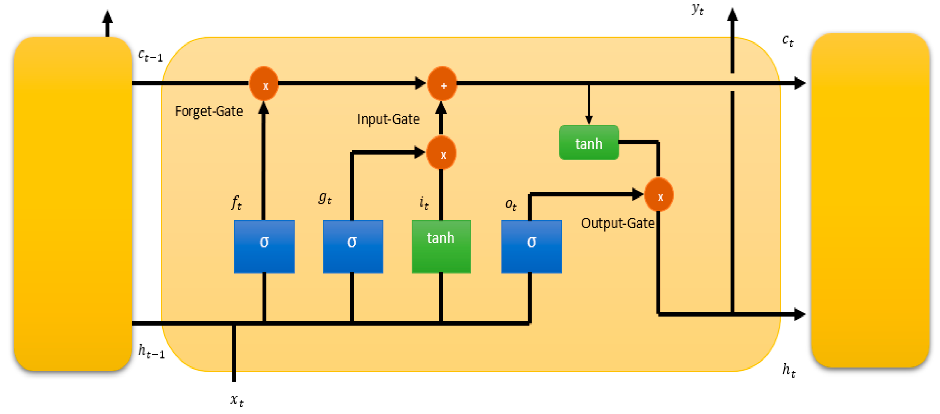
The LSTM network, as shown in Figure 1, has three gates (input, forget and output) for information control, which allows the model to retain and update information over time to enable better modeling of long-term dependencies in sequential data.

Figure 1.
Long short-term memory cell architecture.
The centerpieces of the LSTM cell are the three gates: the input gate, forget gate and output gate. They control the flow of information within the cell. The forget gate, denoted as , uses the previous short-term memory state and the current input to decide which information is discarded from the long-term state. By applying a sigmoid function, the forget gate outputs values between 0 and 1 for each number in the cell state. The resulting value of the forget gate determines the proportion of information from the long-term memory that will be discarded, allowing the LSTM cell to regulate the flow of information through time. Additionally, the LSTM cell includes an additional input, denoted as , representing the long-term state, which is passed along the cell’s operations from one time step to the next time step. This value is used for the calculation of the new long-term state and short-term memory state . The input gate consists of two components. The first component, denoted as , uses a sigmoid function to control the flow of new information into the memory cell. It determines which information from the current input and from the previous short-term memory state is relevant to update the cell state. After determining which values to update, the cell update () computes the new candidate values that will be added to the cell state. This process is carried out using the tanh function, which squashes the values between −1 and 1. The output of the tanh function captures the potential new information that might be added to the cell state. Furthermore, the LSTM cell involves combing the information retained by the forget gate and the new information introduced by the input gate to update the current long-term state , forming a blend of historical information and newly relevant information. In the final step, the output gate calculates what part of the internal state and what part of the long-term state should be passed to the output layer and the hidden state of the next time step. The hidden state of the next time step is influenced by the internal state and the output of the output gate from the current time. Another model for long short-term prediction is LSTNet. This architecture combines convolutional and recurrent layers. The Convolutional Neural Network (CNN) component captures local patterns and short-term dependencies, while the RNN component captures long-term dependencies. It also uses an efficient temporal recurrent skip component to better enable the capture of long-term dependencies [23].
In recent years, Transformer-based approaches have achieved remarkable results in the fields of language processing, computer vision and also forecasting [15,24,25,26].
2.1.2. Transformer
A Transformer model consists of two fundamental parts, the encoder and the decoder, as illustrated in Figure 2. In addition, it contains embedding layers that are responsible for converting the input time series tokens into continuous vector representations. The vector representations are called embeddings. Each input time step is treated as a token, and the embedding layer assigns a learnable vector to represent the features of that input time step. The positional coding is linked to the input time series embedding. There are various options and combinations for carrying out these embedding processes. In this study, there were three different types of embeddings (token, positional and temporal) combined to create a more comprehensive representation of the input data. The token embedding is used to embed the input values. It employs a 1D convolutional layer to capture patterns in the input sequence. The position embedding layer is used to embed positional information in the input sequence. It provides the model with information about the order of elements in the sequence, allowing it to distinguish between different positions. This positional encoding is calculated by using a combination of the sine and cosine functions. Furthermore, the time feature embedding class is utilized, and with the aid of a linear layer, it enables the model to learn the relationships and patterns within the time-related features [27]. This embedding process is employed within both the encoder and the decoder. Furthermore, add & norm blocks occur in the encoder as well as the decoder. These are a combination of residual connections and layer normalization. Residual connections optimize deep model training by ensuring a direct unimpeded path for gradient flow. The normalization layers stabilize the training by normalizing the activations within a layer, preventing the model from exploding or vanishing gradients.
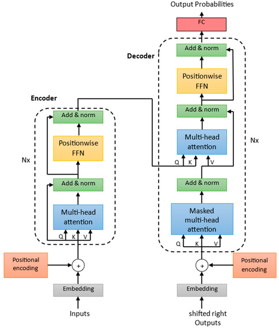
Figure 2.
The architecture of a Transformer.
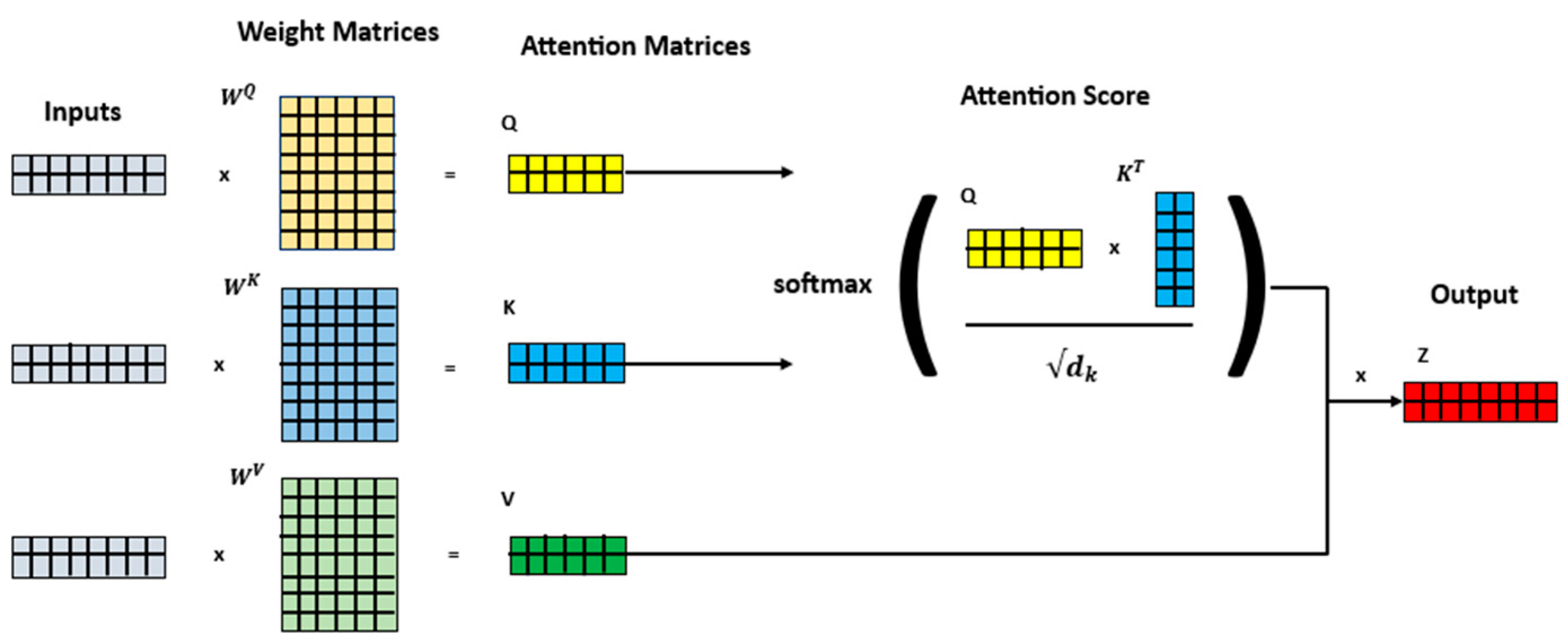
The self-attention mechanism is a key component of Transformer-based approaches, which have revolutionized many application fields. The concept of self-attention allows the model to determine dependency relations between positions within a sequence of inputs. For each encoder input vector, three vectors are associated: the query vector (), key vector (), and value vector (). To speed up the calculation process, the three vectors are plotted in a matric form, where each row corresponds to one input vector. In Figure 3, the expedited calculation process is visually represented through the use of matrix forms for the three previously described vectors. Each row within these matrices corresponds to an individual input vector. Going forward, symbolizes the query matrix, represents the key matrix and stands for the value matrix. In the following, these matrices are multiplied by the corresponding weight matrices ( for each matrix, which are adjusted during the training process and are initially randomly initialized. After the computation of the three matrices, the attention mechanism computes a score between the query matrix ( and the key matrix (, as the dot product divided by the square root of their dimensionality. After this, the scores are normalized by applying the softmax function. Finally, the output is calculated by multiplying the softmax score with the value matrix (. In Figure 4, this process is once again vividly illustrated through the use of blocks. This breakdown into individual blocks illustrates the overall flow. The resulting scores determine the degree of attention placed on other parts of the input sequence when processing a specific element of the token at a given position. In this process, important values are highlighted, and less relevant values become small [26].

Figure 3.
Illustration of the calculation of an attention head, which is computed in the multi-head attention block of the Transformer architecture.
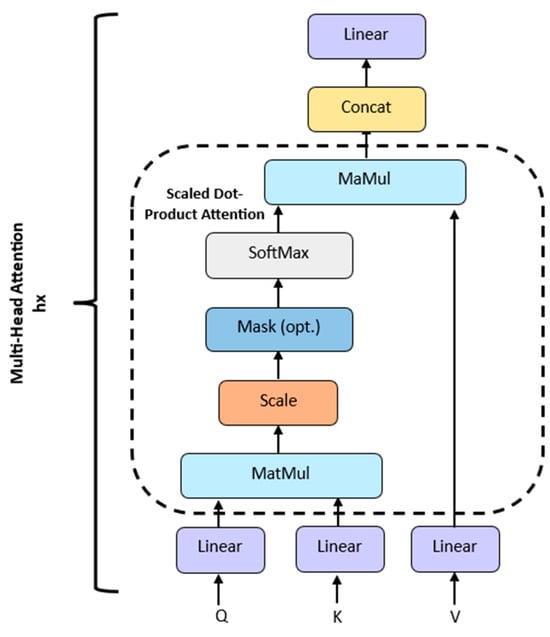
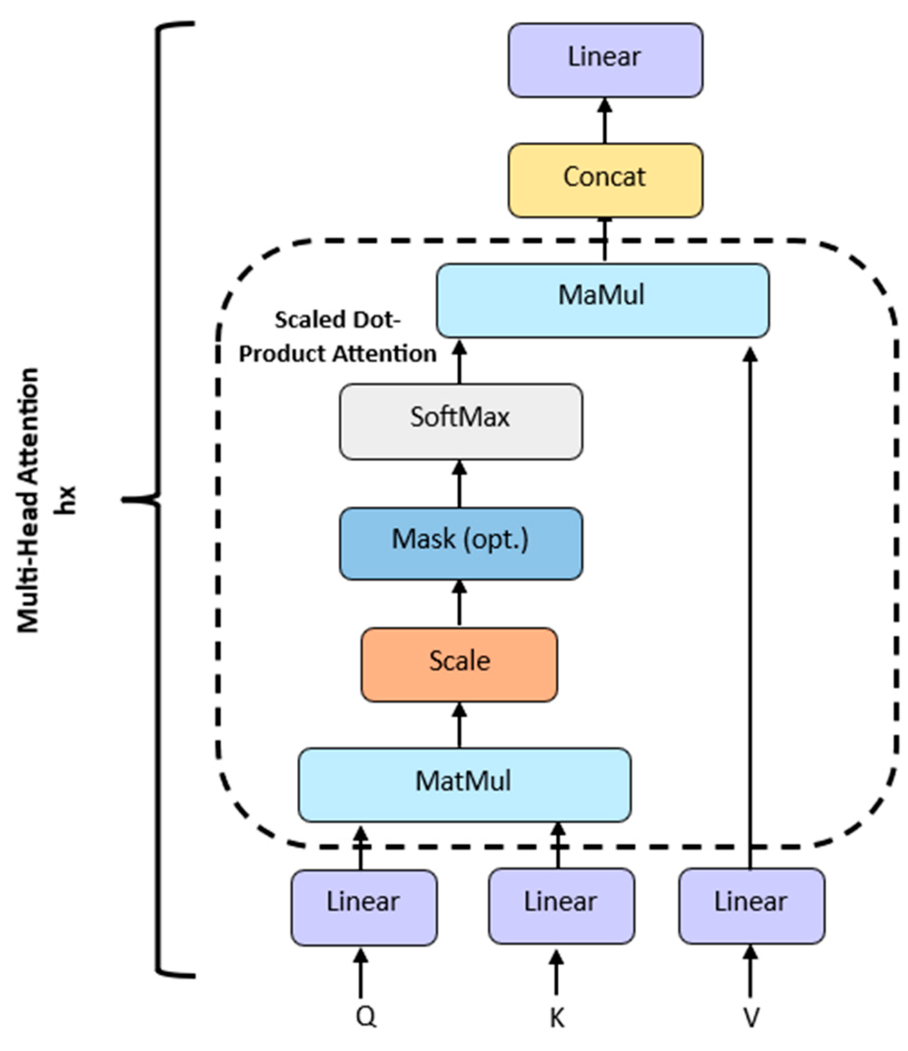
Figure 4.
Explicit representation of the processes in a multi head attention block. The term “multi-head” means that the self-attention mechanism is applied times in parallel. Each head independently learns various patterns.
The term ‘multi’ refers to the use of multiple attention heads to capture diverse temporal patterns and dependencies. This enables the model to learn different aspects of temporal relationships simultaneously. The attention mechanism described above also applies to the decoder, with the difference being that a mask is applied to the score to prevent the decoder from attending to future knowledge. The concept that important information is highlighted and less relevant information becomes unimportant is also used in TCNN-based [28,29] and RNN-based [30,31] approaches; for example, spatiotemporal self-attention-based LSTNet uses two self-attention strategies. Temporal self-attention determines the relative importance of historical data for predicting future outcomes by calculating the correlation scores between each historical datapoint and the predicted values. Spatial self-attention calculates the impact of various features on the output. Important features are weighted higher, and less important features are weighted lower [31]. In the following, the focus will be on Transformer-based approaches.
2.1.3. Informer
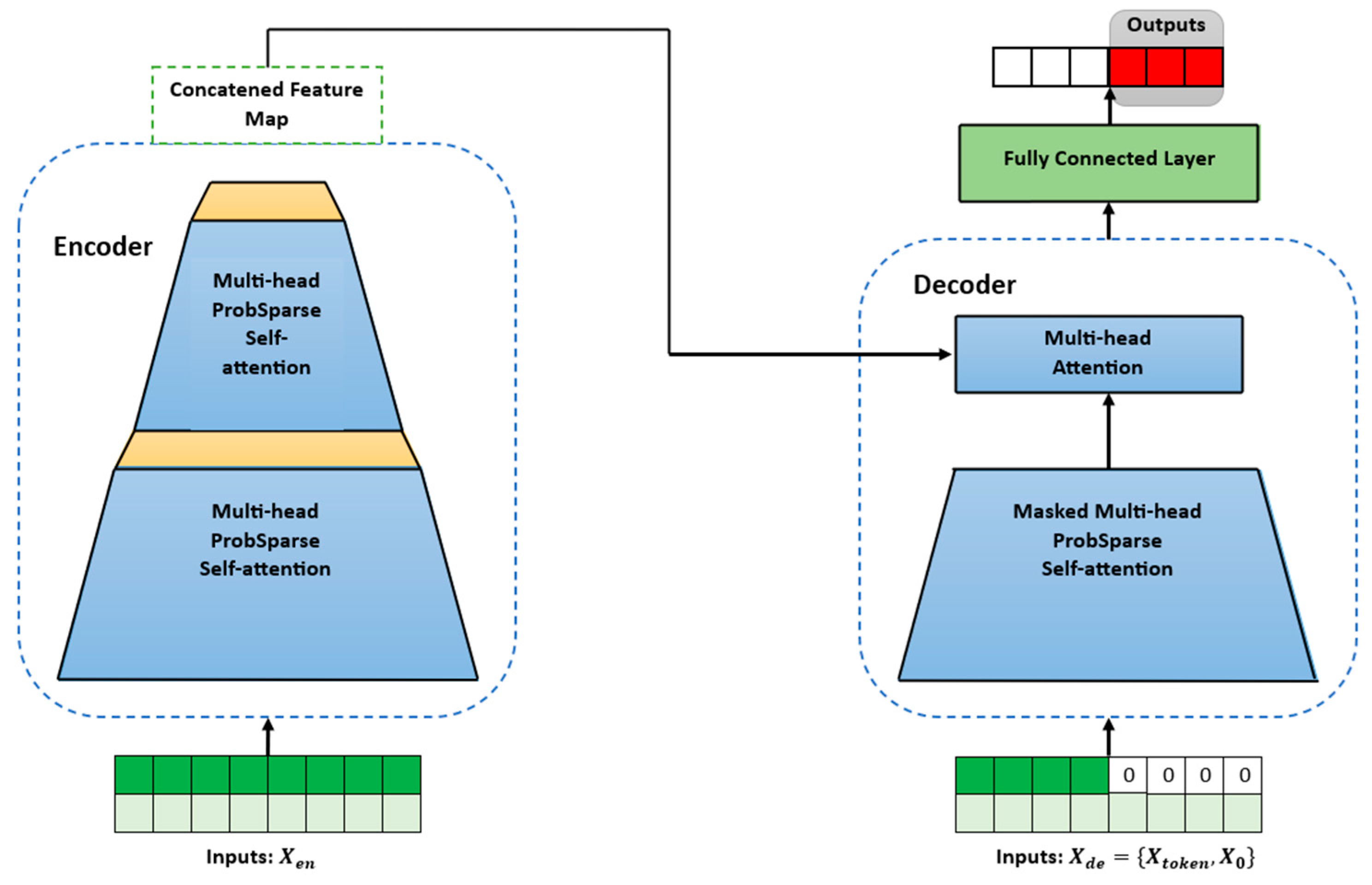
The Informer architecture is specifically designed for long-term forecasting. As illustrated in Figure 5, the Informer model is composed of an encoder and a decoder. Informer uses a probabilistic (prob) sparse self-attention mechanism instead of a canonical self-attention mechanism. This change reduces the time complexity and memory usage per layer, which is significant for solving long-term forecasting [15]. This reduction in time complexity and memory usage is achieved by using a subset of queries to calculate the score in the prob sparse self-attention. The most relevant subset is determined by a probability measurement, the Kullback–Leibler (KL) divergence. The KL divergence is a statistical metric that measures the dissimilarity between a given probability and a reference probability distribution. In the prob sparse self-attention mechanism, the KL divergence is used to quantify how diverse or focused the attention probabilities are for a given query. In other words, the KL divergence is the basis of the sparsity measurement. It selects the likely most informative queries based on their attention probability distributions. A more diverse distribution means that the query is more informative, while a focused distribution implies that the query is less informative and can therefore be discarded for further calculations. This approach allows the Informer model to selectively attend to queries based on the diversity of their attention distributions, and more likely informative queries are used for calculating the output of the self-attention layer.

Figure 5.
The architecture of an Informer.
As a result of the prob sparse self-attention mechanism, there could be redundancy in the feature mapping. This redundancy may arise from combinations of values that represent the same trend or pattern in the provided data. To address this redundancy, the Informer model uses a distilling operation. This operation aims to reduce the redundant information and assign higher weights to the dominant features in the output of the respective attention block. Figure 6 provides a detailed illustration of the process in an encoder stack.

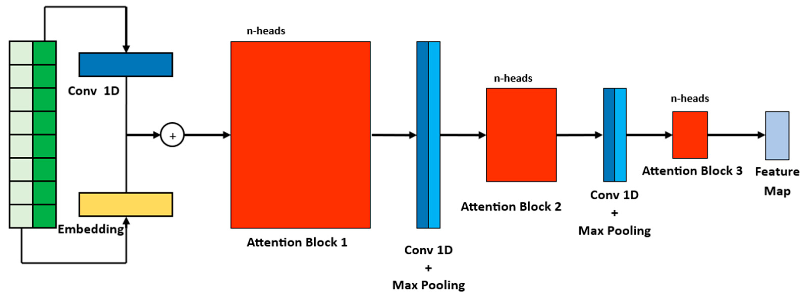
Figure 6.
Inner stack architecture of an encoder. The notation -heads, like in the Transformer model, means that the self-attention is applied times in parallel.
2.1.4. Autoformer
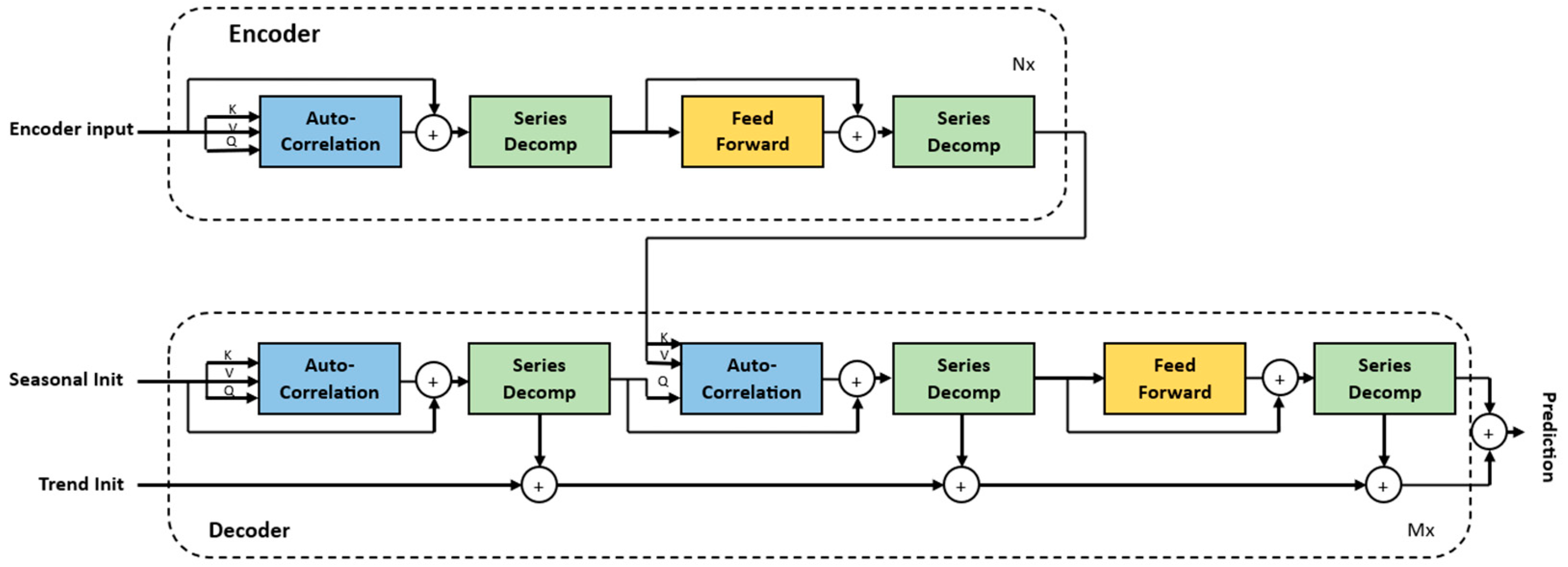
As illustrated in Figure 7, the Autoformer model adopts a different approach than the previous Transformer models, based on decomposition and autocorrelation. The decomposition of time series is a technique used to disassemble time series data into their component parts. The primary components that the decomposition block of the Autoformer model disassembles from the time series data are trend and seasonality. The goal is to discern underlying patterns within the data, such as considering seasonality in the context of predicting energy from PV sources to resolve hourly, daily, monthly or yearly patterns, or considering long-term patterns (trend component) to determine whether the time series or certain periods exhibit an increase or a decrease or remain relatively stable over time. Series decomposition is performed as an inner block of the encoder and decoder, where the input series are split into the seasonal part and the trend-cyclical part. First, the encoder focuses on the extraction of seasonal components by eliminating the trend component. The extraction of the trend cycle is achieved by applying a moving average with padding to the input data, in order to smooth out periodic fluctuations. Consequently, the seasonal part is attained by subtracting the extracted trend cycle part. Then, the resulting periodicity is utilized by the auto-correlation mechanism to group similar periods from other sub-time series. Finally, this seasonal information is passed, as cross-information, to the decoder so that it can further refine the prediction. In comparison to the two other Transformer models, the Autoformer model replaces the self-attention mechanism with auto-correlation. The decoder consists of an upper branch and a lower branch, which comprise the accumulation part of trend-cyclical parameters and a stacked structure for seasonal components. The upper branch is a stacked structure to capture seasonal components, which initially employs auto-correlation to capture the inherent temporal dependencies present in the predicted future states. Subsequently, it leverages historical seasonal information from the encoder to decipher specific dependencies and refine the forecast. The auto-correlation block identifies dependencies by calculating the series autocorrelation and aggregates similar subseries through time-delay aggregation [16]. Subseries that share a common periodicity are considered similar, and time-delay aggregation is a technique used to combine multiple of such subseries into a unified representation.

Figure 7.
The architecture of an Autoformer.
2.1.5. FEDformer
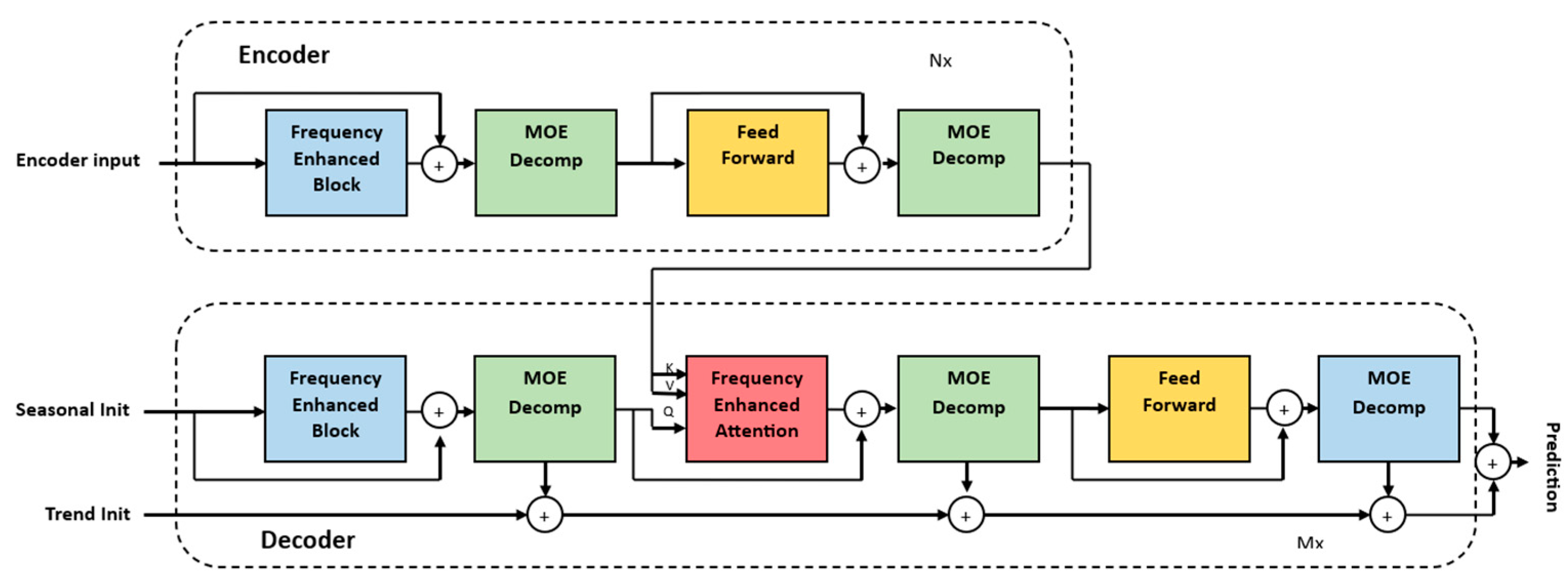
Like the Autoformer model, the FEDformer model uses seasonal-trend decomposition to identify global properties. The FEDformer model has a similar structure to the Autoformer model. However, it does not consist of three main blocks like the Autoformer model; instead, it consists of four main blocks: frequency-enhanced block (FEB), frequency-enhanced attention (FEA), feed-forward network and mixture of expert decomposition (MOEDecomp). The purpose of the FEB blocks is to discern crucial patterns within time series by integrating insights from the frequency domain. Within the domain of FEB, there exists a categorization into two variants: Fourier-enhanced block and wavelet-enhanced block. The FEDformer model uses high- and low-frequency components to represent the time series. Wavelet and Fourier transform are used in signal processing and analysis to represent signals in different domains. Applying Fourier transform to our time series yields the frequency resolution of the data, but it does not convey how these frequencies evolve over time. In contrast, wavelet transform can capture the frequency and the time information of the time series. It can capture both high- and low-frequency components at different points in time. In contrast to Fourier transform, the data do not have to be stationary. In the context of wind energy forecasting, weather parameters like wind speed and direction are dynamic and can rapidly change. Using Wavelet transform can help capture the varying frequency components of a possible non-stationary time series over time, providing more accurate information for forecasting models. FEDformer employs a strategy of randomly selecting a fixed number of frequencies. This approach serves to mitigate the challenges associated with linear storage and calculation costs, while also addressing the potential issue of overfitting. By utilizing a fixed number of frequency components, the model’s ability to generalize increases. As with FEB, FEM has two variants. In FEA with Fourier transform, the conventional queries, keys and values utilized in the canonical attention mechanism in the standard Transformer model undergo a modified attention process. This modification involves applying an attention mechanism in the frequency domain using Fourier transform. MOEDecomp is an advanced method designed to extract the trend component from a time series that exhibits a periodic pattern [17]. This approach utilizes a set of average filters with varying windows sizes, enabling it to capture different aspects of the underlying trends. By employing multiple filters, MOEDecomp can identify and isolate various trend components within the time series. This process is depicted in Figure 8 in the lower branch of the FEDformer decoder.

Figure 8.
The architecture of a FEDformer.
2.1.6. Non-Stationary Transformer
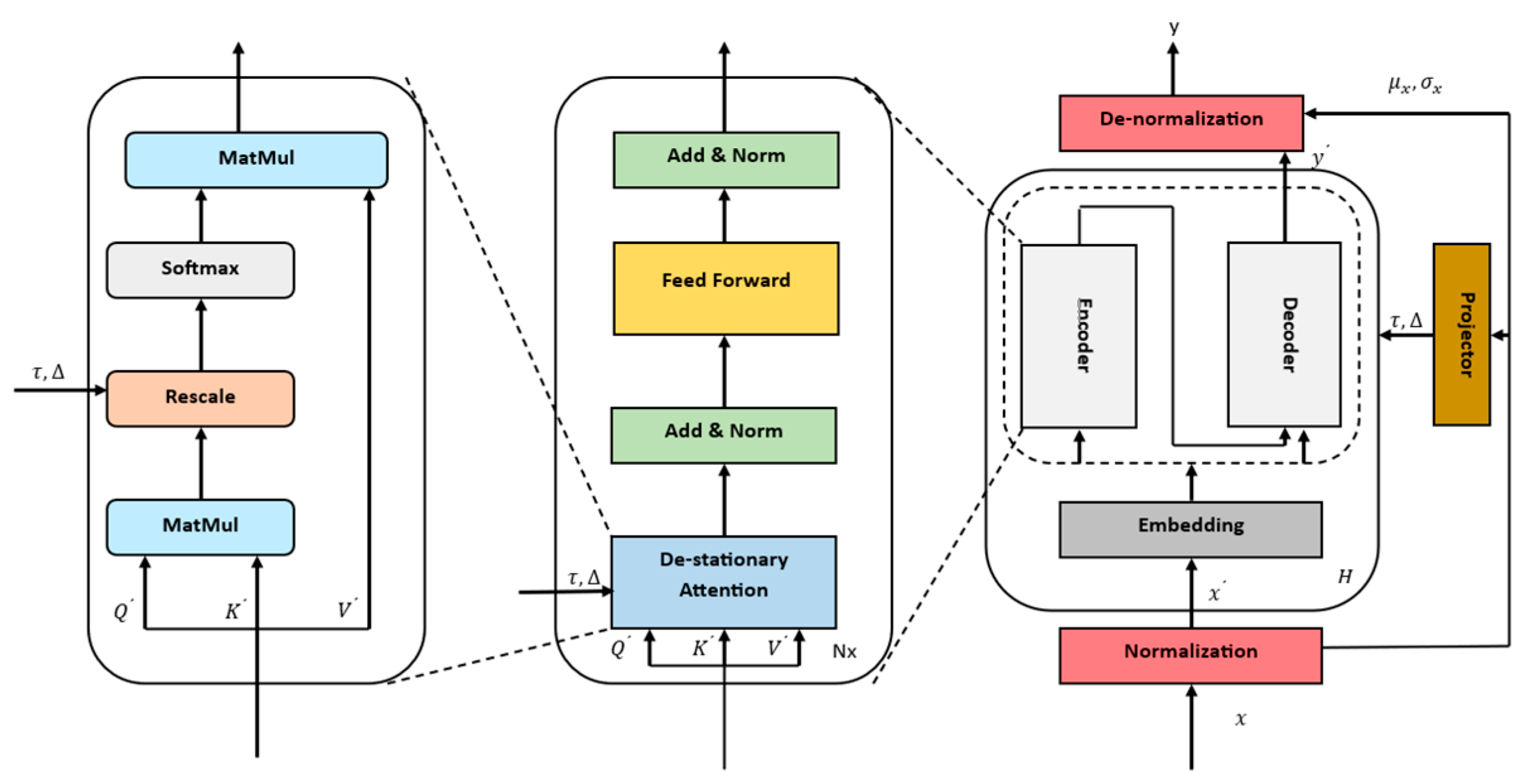
The architecture of the Non-Stationary Transformer model is depicted in Figure 9. The essential core elements of the non-stationary model are the normalization block and the de-stationary attention block. The fundamental idea of the normalization block is to normalize each incoming time series at the input and de-normalize the model output. The normalization block normalizes each input time series by adjusting its mean ( and standard deviation (, giving it a more stable and normalized distribution of the model input. The de-normalization module is applied after the Base of the model. The aim of the de-normalization module is to reverse the normalization process applied to the model output during the inference phase, taking into account the statistics represented by and . The Non-Stationary Transformer model counteracts the problem of over-stationarization by de-stationary attention. The over-stationarization problem leads to indistinguishable attentions and the loss of crucial temporal dependencies in the deep model [18]. Classical models like ARIMA apply differencing to make the time series stationary. This can lead to over-stationarization if too much effort is made to make the time series stationary, as important information can be lost and it is no longer possible for the model to establish an existing relationship. The objective of the de-stationary attention block is to reintegrate the non-stationary information that was omitted during the stationarization process, thereby restoring the lost information and improving prediction performance. To achieve this, the de-stationary factors and are introduced. is a positive scaling factor and is calculated using a multilayer perceptron (MLP) based on the standard deviation of non-stationary data . is a shifting vector and is calculated using a MLP based on the mean of the non-stationary data . The attention score is calculated in exactly the same way as for the standard Transformer, except that the de-stationary attention uses de-stationary factors to rescale the temporal dependency weights.

Figure 9.
The architecture of a Non-Stationary Transformer.
2.2. Data
The data on electricity generation come from the information platform SMARD, which is provided by the German Federal Agency Bundesnetzagentur [32]. SMARD contains all important data about the electricity market, electricity generation and electricity demand. The weather information comes from The German Weather Service (DWD). The DWD has more than 2000 weather stations. The DWD offers free access to the Climate Data Center (CDC) [33]. The CDC portal provides visualizations of current metrological weather data in Germany and offers access to diverse climate data. The CDC database provides, depending on the weather station, different temporal resolutions for 15 meteorological weather parameters.
2.3. General Preprocessing
In the forecasting analysis, the time period from 1 January 2015 to 31 December 2021 was taken into account. The electricity generation data from SMARD are available at a resolution of 15 min. To form hourly data points, the 15 min data intervals were summed up. The next step was anomaly detection. The anomaly detection was performed using an Isolation Forest, which builds a random forest based on decision trees. Additionally, the data were examined for missing or erroneous values. Erroneous measurements in the weather data were marked with −999 or −99. These values were removed or interpolated. The individual data points were checked for stationarity using the ADF test. The ADF test is a unit root test that determines, based on a null hypothesis, whether a time series is stationary or non-stationary. As long as the p-value is ≤ 0.05, the null hypothesis is rejected, indicating that the time series is stationary. According to the test result, the data were stationary. Stationarity is a crucial assumption for traditional models like ARIMA and SARIMA. While powerful deep learning models, like CNN, LSTM and Transformers, are capable of handling non-stationary data to some extent, they often perform better when the data are stationary or have certain stationary properties. For example, RNNs and LSTMs are designed to handle sequential data, where the order of data input matters. Furthermore, they have the ability to selectively forget or recall information based on the significance of previous occurrences. They can recognize temporal relationships and accumulate knowledge about patterns. This makes them well suited for non-stationary data. Subsequently, the data were standardized and transformed into their model form.
2.4. PV
The following section describes the data preparation and implementation for the prediction of electricity generation by photovoltaics.
Preprocessing and Data Overview
The weather stations were selected according to a specific scheme. Firstly, the largest installed capacity was selected and sorted by federal state. Figure 10 shows a pie chart with the share of the maximum installed capacity of the various federal states. The installed capacity by federal state serves as the basis for the selection of weather stations. The pie chart shows that more than 1/4 of the installed capacity is located in Bavaria. Furthermore, approx. 40% of the installed PV capacity is located in south of Germany, and 67% of the installed PV capacity is located in six federal states.
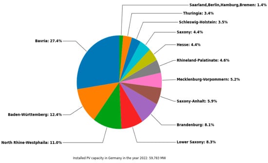
Figure 10.
Installed PV capacity by federal state in 2022.
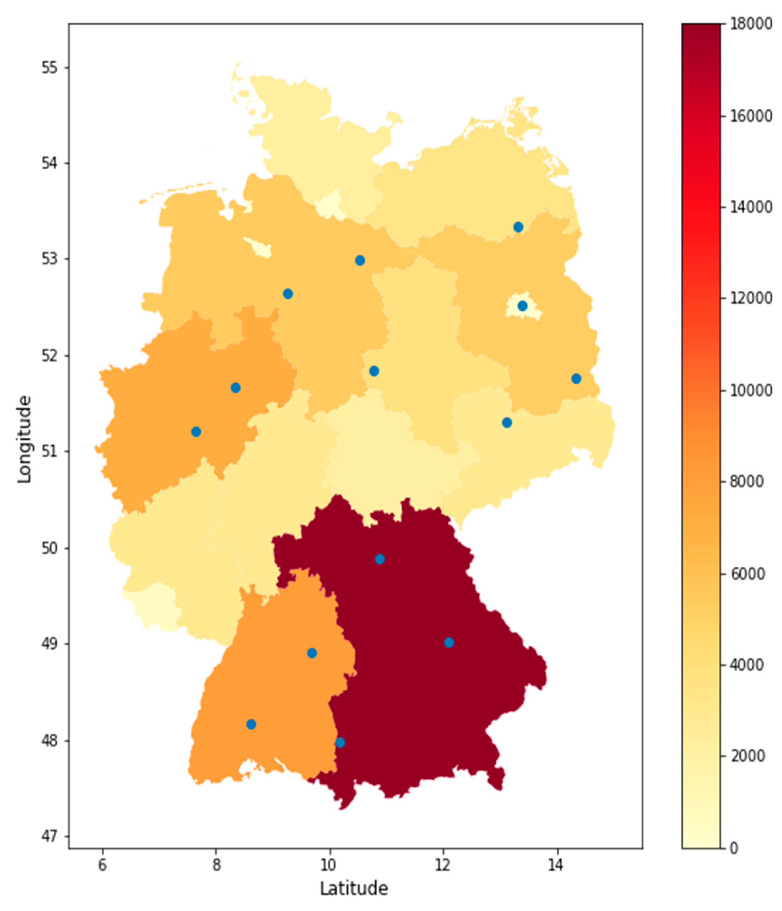
After determining the distribution of the installed PV power, the locations of the PV systems within each respective federal state were determined. The selected weather stations should ideally contain a wide radius that contains PV systems. The majority of federal states have an energy atlas that shows the various installed renewable energies. In addition, the energy atlas includes many other important factors, such as annual average solar radiation or promising locations for renewable energy. All open accessible weather stations and their information were taken from the DWD Weather Station encyclopedic and loaded into a pandas data frame. The data frame comprises information about the weather station location and the period of the weather records. Additionally, abbreviations indicate the parameters measured by the weather station. Figure 11 shows the selected weather stations based on the described procedure. For some weather parameters, weather stations were selected near the marked position in Figure 11. The reason for this is that it is difficult to find weather stations that collect all weather parameters. All weather parameters from the marked weather stations were attached to a data frame and the mean value was calculated for each parameter. It is important to mention that, especially in the case of PV, this process cannot be standardized. When examining the individual areas where, for instance, PV modules are installed, e.g., in Bavaria, one comes to the realization that the PV modules are spread comprehensively across the entire state. Especially noteworthy is that the development of installed PV modules is on the rise. This method is intended for the generalization of this extensive subject. The described approach, which places the installed PV capacity of each federal state at the forefront when selecting weather stations as criteria, aims to choose weather stations as representatively and in as comparatively simplified a manner as possible. The aim is to describe the entire electricity generation from PV in Germany at a national level. Using installed PV capacity as a criterion is reasonable as it reflects the actual generation potential in each federal state. This prioritization of regions with higher production of solar energy is essential in order to make the broadest possible generalization. Considering a generous radius around selected weather stations is a strategy aimed at capturing the spatial variability of solar energy resources within a federal state. With such a large generalization solution, there are some limitations to the proposed approach. The proposed approach operates under the assumption that the installed capacity reliably reflects the true solar energy potential. However, this assumption may not hold universally, as factors such as fluctuations in solar panel efficiency, orientation and the impact of shading can introduce variations in actual solar energy generation. This argument can be partially invalidated by using the aforementioned energy atlas, which, among other things, provides information on which areas in a federal state have particularly favorable conditions for locating a PV system. However, it is important to note that a possible limitation of this approach (when selecting a certain number of weather stations) is that microclimates can influence the selected weather data. There is also another approach for determining how to deal with the weather parameters. One approach could involve including additional weather stations and calculating the mean or weighted values in relation to the installed capacity of each federal state.

Figure 11.
Selected weather stations and installed PV capacity by federal state in 2022. The blue dots represent the location of the selected weather stations.
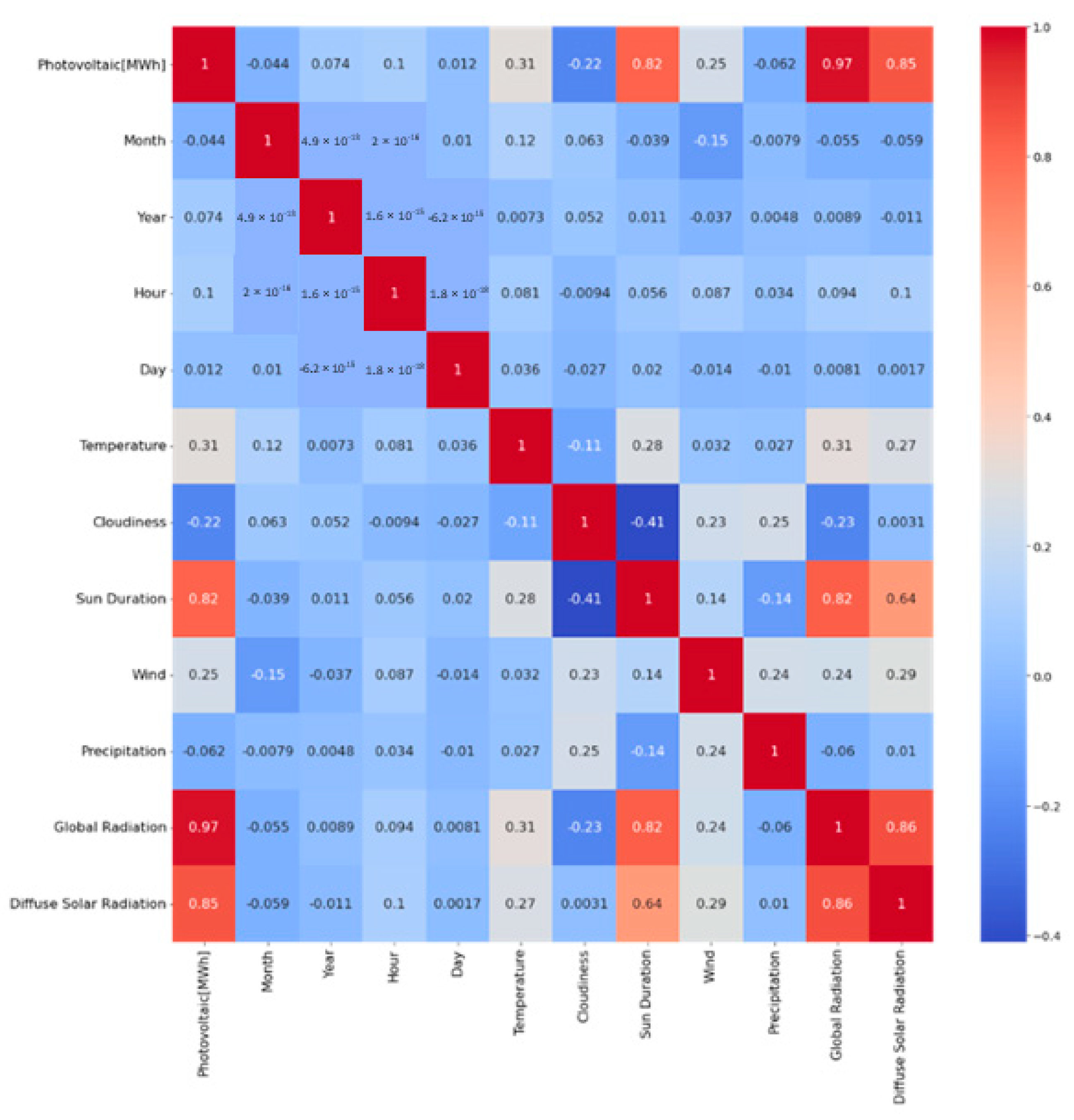
Figure 12 shows a heatmap with the correlations between the respective parameters. The Pearson correlation coefficient was used for the calculation. The Pearson correlation coefficient is a measure of the linear relationship between two variables. It ranges from −1 to 1, where −1 indicates a perfect negative linear correlation, and 1 indicates a perfect positive correlation. As excepted weather parameters, such as diffuse solar radiation, global radiation and sun duration are very important for power generation. Cloudiness has a negative correlation of −0.22 with the power generated by photovoltaics. This implies that greater cloud cover reduces the power generation. Furthermore, wind has a correlation of 0.25 and temperature has a correlation of 0.31 with the power generated by photovoltaics. In addition, an analysis was carried out using the Spearman correlation coefficient. The Spearman rank correlation coefficient is a non-parametric measure of statistical dependence between two variables. Unlike the Pearson correlation coefficient, which measures linear relationships, the Spearman’s rank correlation rates the monotonic relationship between two variables, which means it detects whether there is a consistent trend in their association, even if it is not linear. The Spearman rank correlation coefficient, like the Pearson, emphasizes the strong positive correlation (>0.90) between sunshine duration, global radiation, diffuse solar radiation and energy generation from photovoltaics. It is crucial to remember that correlation does not necessarily imply causation.
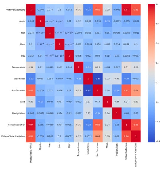
Figure 12.
Pearson correlation map for PV of the different values (weather parameters, time).
In the comparative study conducted, two different approaches to the selection of weather parameters are considered. In the first approach, all the weather parameters depicted in Figure 12 and time specifications such as month and hour are taken into account for the prediction. Meanwhile, the second approach focuses on using a subset of selected weather parameters. In the second approach, the weather parameters with the highest correlation are chosen. These parameters are sunshine duration, global radiation and diffuse solar radiation.
Figure 13 confirms the previous assumption. It shows the mean PV electricity generation for each respective month and hour. The mean value was computed by averaging the combination of all the data for each time window (month, hour) for the period from 2015 to 2021. During the midday hours in spring and summer, the photovoltaic systems produce the most energy. This is the case, for example, when there is a significant amount of direct global radiation and on days with many hours of sunshine. It shows seasonality over the year and daily periodicity.
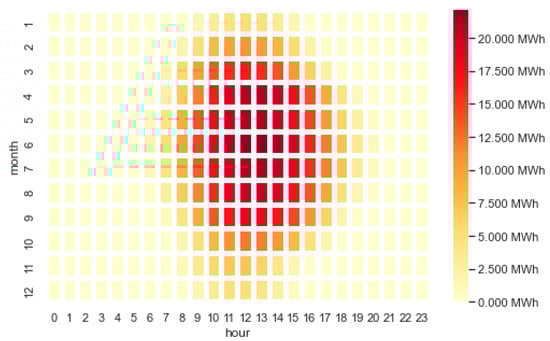
Figure 13.
Heatmap of mean electricity generation depending on hour and month.
2.5. Onshore Wind
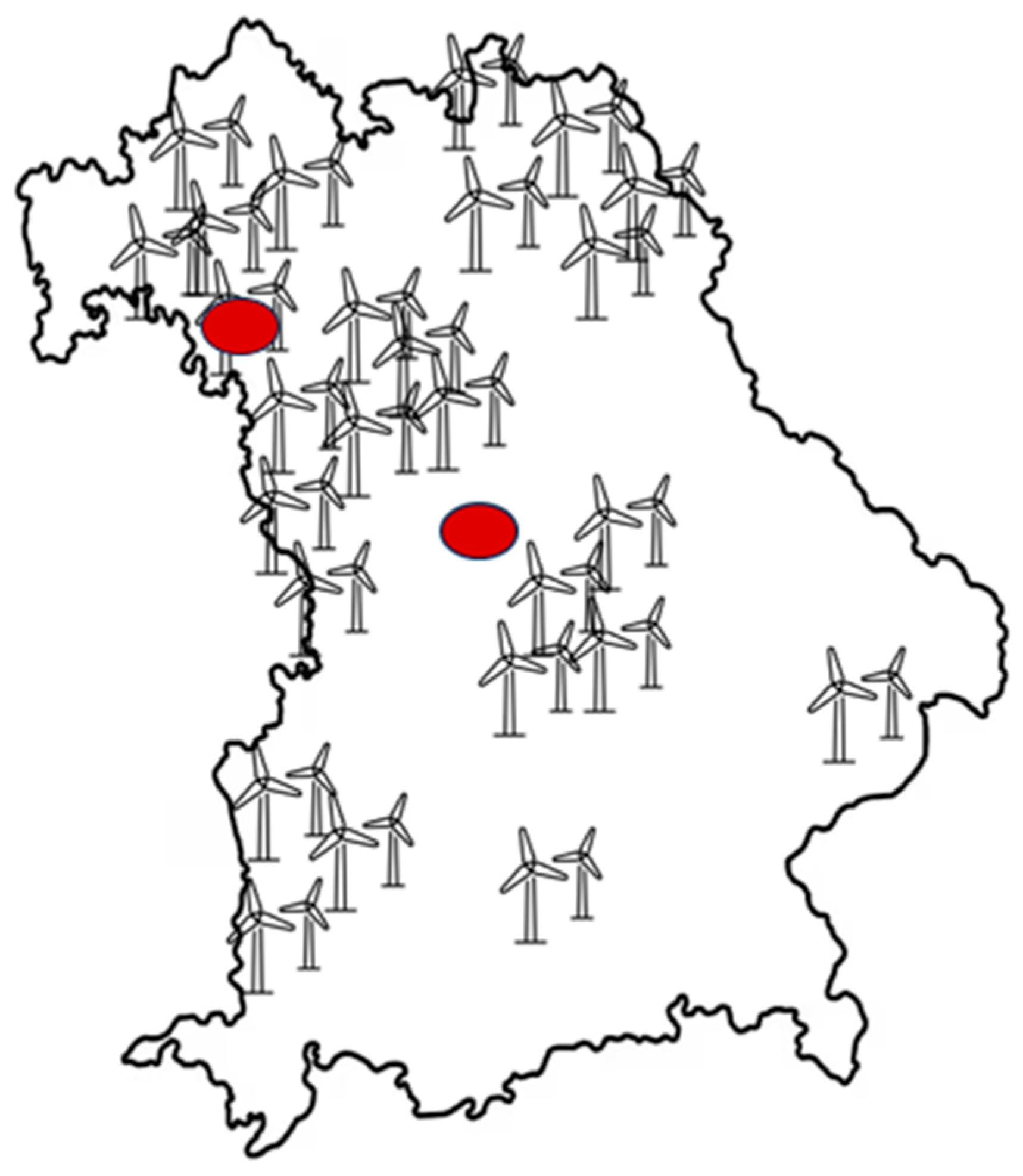
The following section describes the data preparation and implementation for the prediction of electricity generation by onshore wind turbines. The processing of data occurred in the same way as described in Section 2.4 Figure 14 visually depicts the previously described method for finding the weather stations, utilizing an example set of the approximate density of installed wind turbines in Bavaria. The density of the wind turbines was not precisely determined, but roughly estimated using the Bavarian energy atlas [34]. This merely serves to illustrate the method described compared to the chosen used method in Section 2.4 The same advantages and disadvantages apply to the chosen method as to PV. Here, specific elements related to onshore wind, such as wind turbine, rotor diameter, etc., have an influence. This section provides an overview of the onshore wind turbine data.

Figure 14.
Map of the federal state of Bavaria. Wind turbines show the approximate density. Red circles indicate the approximate location of the selected weather stations [32].
Data Overview
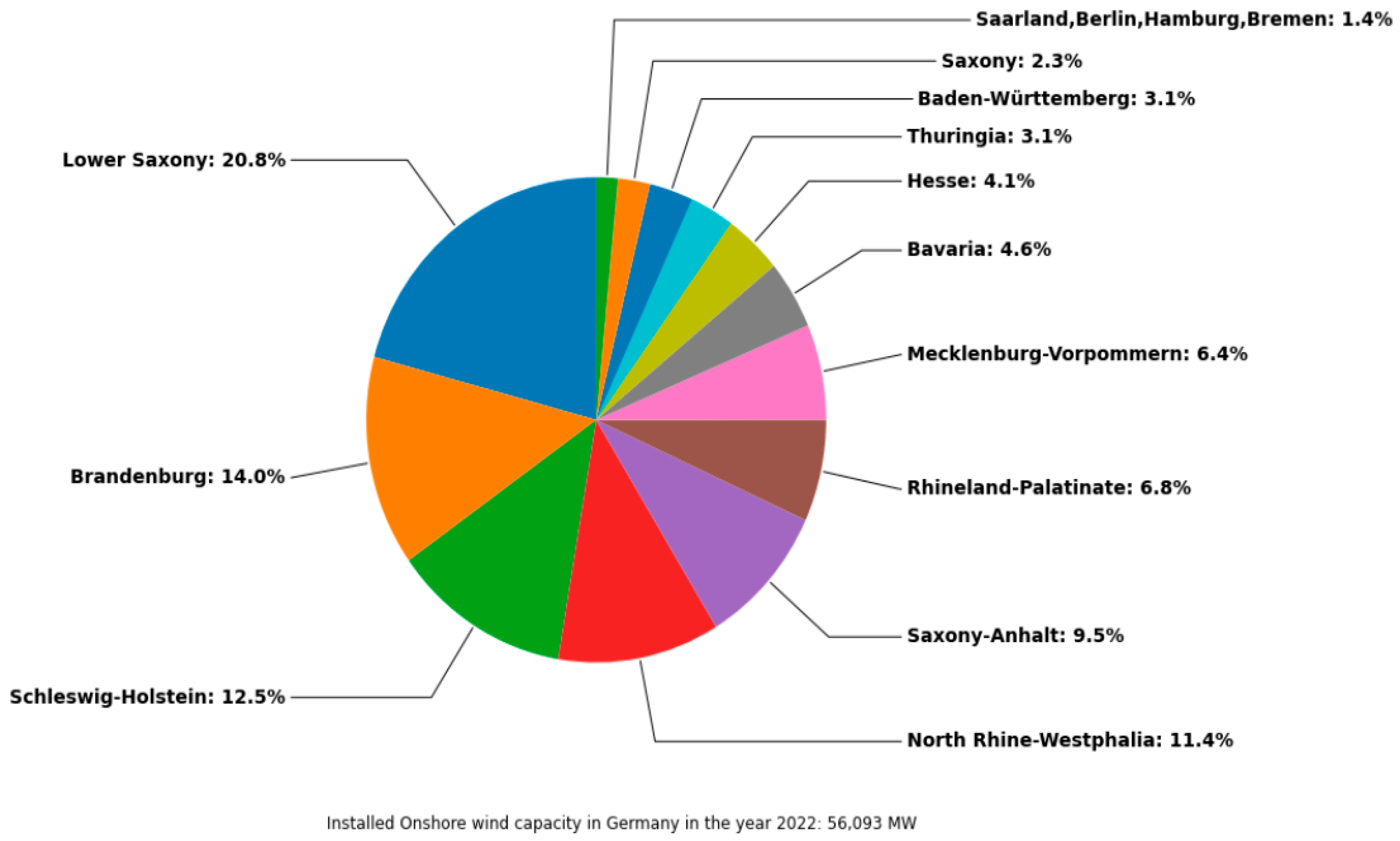
Figure 15 shows a pie chart with the share of the maximum installed capacity of the various federal states. The installed capacity by federal state serves as the basis for the selection of weather stations. This time, the focus of the installed onshore wind capacity is on the north. The pie chart shows that 20,8% of the installed capacity is located in Lower Saxony. Furthermore, more than 50% of the installed onshore wind capacity is located in the north of Germany. As a result, the majority of the weather stations are selected in the north. This is evident in Figure 16, where the figure shows the selected weather stations based on the previously described procedure.

Figure 15.
Installed onshore wind capacity by federal state in 2022.
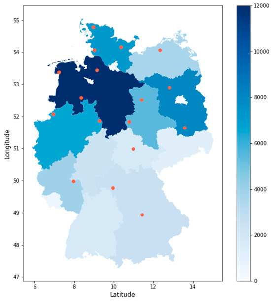
Figure 16.
Selected weather stations and installed onshore wind capacity by federal state in 2022. The orange dots represent the location of the selected weather stations.
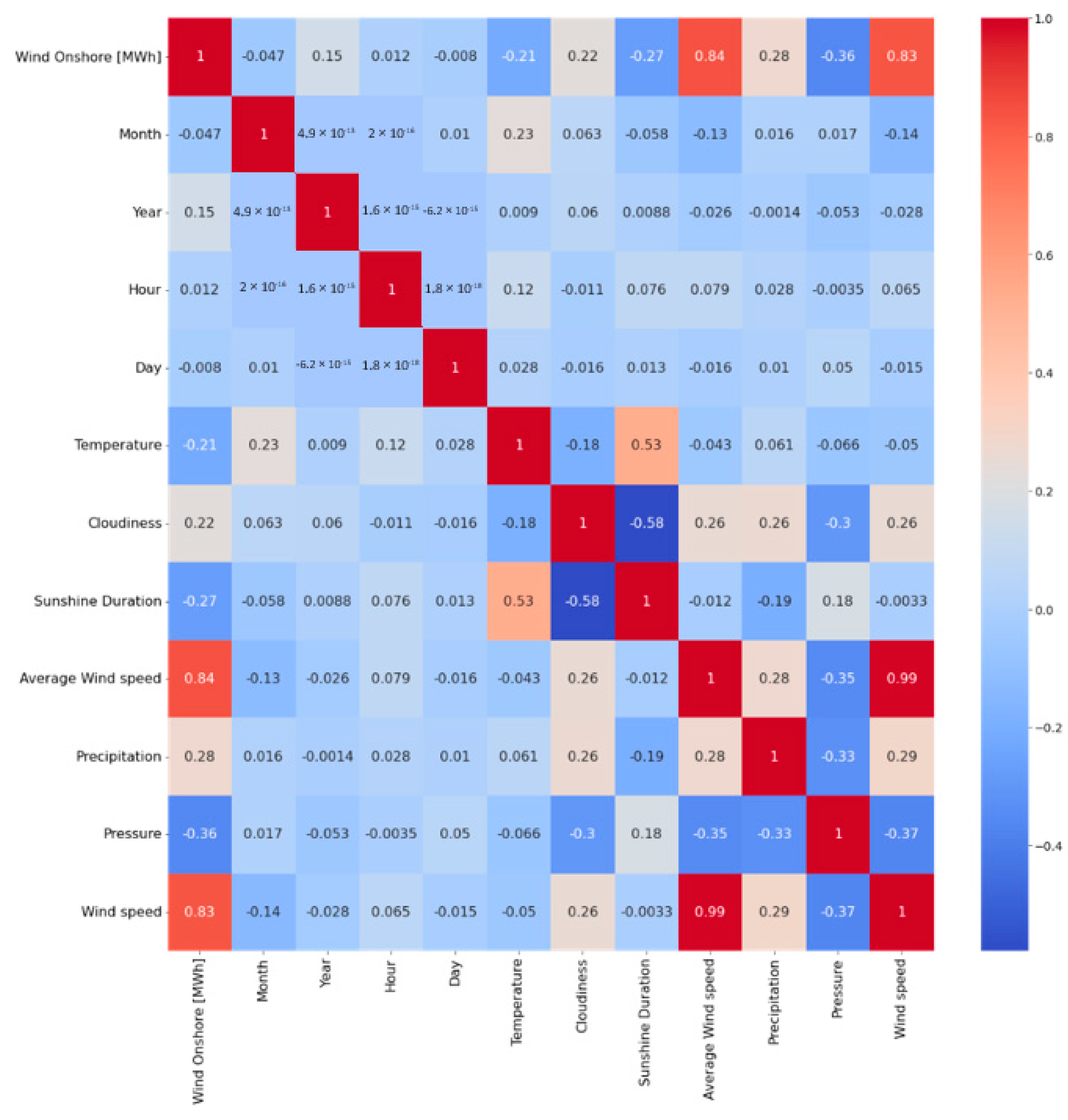
Figure 17 presents a heatmap illustrating the correlation between the respective parameters. As in the PV approach, the correlation was calculated using the Pearson correlation coefficient. Weather parameters such as average wind speed are highly correlated with power generation. This also confirms the analysis with the Spearman correlation rank coefficient. Also, weather parameters like sunshine duration, temperature and pressure are negatively correlated with onshore wind [MWh]. Like in the PV approach, in the first approach, all weather parameters were taken into account for the prediction. In the second approach, the weather parameters with the highest correlation were chosen. These parameters are the wind speed and the average wind speed. The average wind speed is moderately correlated with precipitation and cloudiness. It is also negatively correlated by −0.37 with pressure. However, these weather parameters were not used in the second approach.
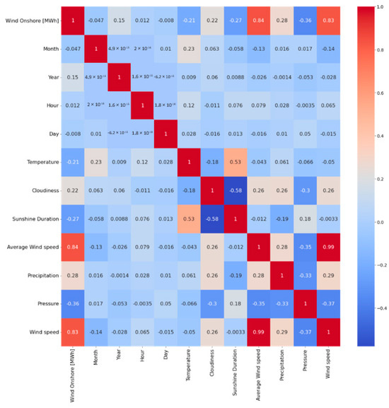
Figure 17.
Correlation map of the different values (weather parameters, time).
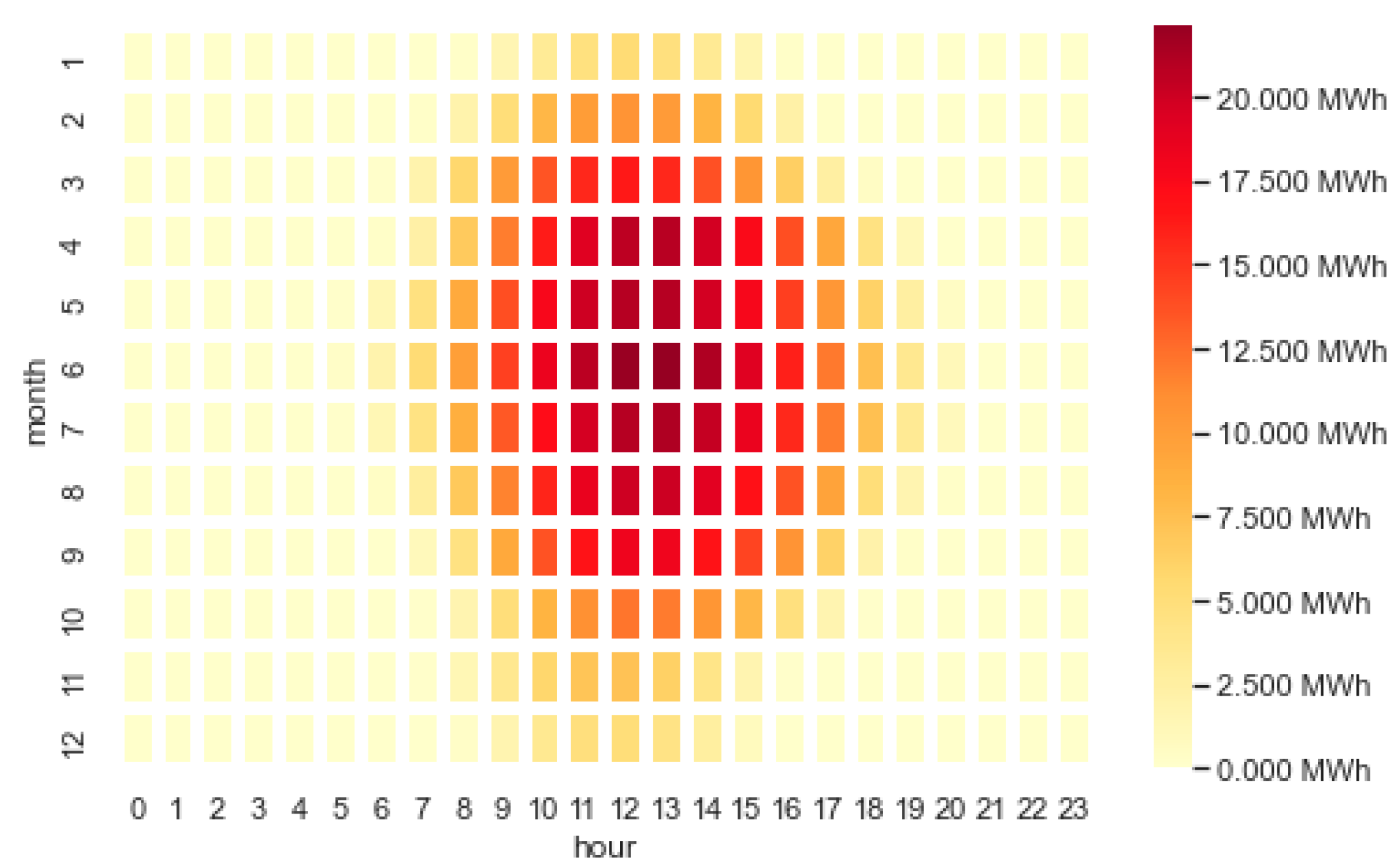
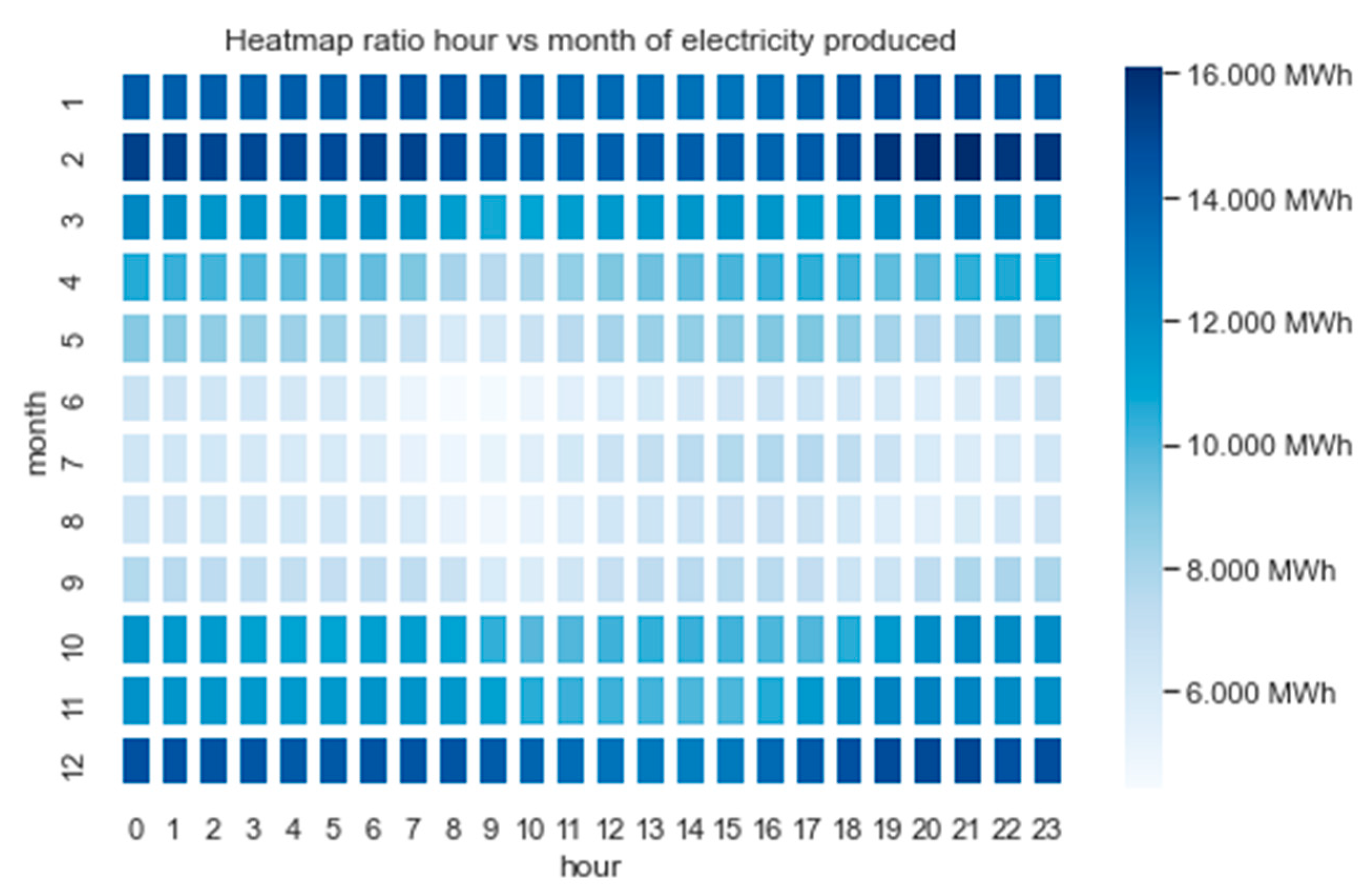
Figure 18 presents a heatmap illustrating the ratio of electricity produced by hour and month. Following the same approach used for PV data, the average electricity generation was calculated for each respective month and hour within the considered period from 2015 to 2021. During wintertime, the onshore wind turbines produce the most energy. From this, one can interpret that the electricity production from onshore wind power indicates more complex statistical properties than electricity from photovoltaics. This clearly shows yearly seasonality, but there are several fluctuations independent of the annual seasonality.
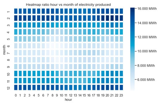
Figure 18.
Heatmap mean electricity generation depending on hour and month.
3. Methodology and Results
This study included the following five Transformer models: Transformer, Informer, Autoformer, FEDformer and Non-Stationary Transformer. In addition, the LSTM- and ARIMA-based models were compared. For onshore wind forecasting, ARIMAX was used, and for PV prediction, SARIMAX was employed due to its seasonal patterns. To determine the parameters of these models, the Autocorrelation Function (ACF) and Partial Autocorrelation Function (PACF) were employed. These functions assist in determining the necessary adjustments for time series data by identifying the appropriate order of differencing (d value); the autoregressive (AR) component (p-value), which looks at past data values to understand their influence; and the moving average (MA) component (q-value), which assesses the impact of past forecasting errors and the seasonal patterns. Once the individual parameters were identified, the Akaike Information Criterion (AIC) score was used to select the optimal model order. The AIC score is valuable for model selection because it aids in finding an equilibrium between the complexity of a model and its capacity to fit the data effectively. By minimizing the AIC score, we aim to find the most parsimonious model that adequately captures the underlying patterns in the data, resulting in accurate and reliable forecasts for renewable energy generation. In the context of wind energy prediction, an ARIMAX model with the order (1,2,1) was selected, indicating a first-order autoregressive component, two orders of differencing for stationarity and a first-order moving average component. In the case of PV, a SARIMA Model with the order (1,0,0) and a seasonal order of (1,0,0,24) was selected. For the LSTM model, various model architectures were attempted, but ultimately, the approach that proved most effective involved utilizing a maximum of three hidden LSTM layers, complemented by dropout layers and L2 regularization, to reduce overfitting and improve model stability. Table 1 provides an overview of the parameters.

Table 1.
LSTM architecture overview. Photovoltaic (PV), long short-term memory (LSTM).
In this paper, the FEDformer, Informer, Autoformer and Transformer models were implemented by utilizing the code provided in the GitHub repository available at https://github.com/MAZiqing/FEDformer, accessed on 15 October 2023 [35], and the Non-Stationary Transformer model was implemented by utilizing the code provided in the GitHub repository available at https://github.com/thuml/Nonstationary_Transformers, accessed on 15 October 2023 [36]. FEDformer-w uses Wavelet transform. Table 2 provides an overview of the parameters that where selected in general for the different Transformer models. Numerous combinations of parameters were explored during the training and evaluation processes of various Transformer models to optimize the model performance. However, the parameters listed in Table 2 demonstrated the most consistent performance in our study.
Table 2.
Overview of the selected parameters that represent the foundational aspects of the five Transformer models. Photovoltaic (PV).
For the investigation, the data were divided into 70% for training and 15% each for validation and testing. For all experiments, the input length was set to 100. The comparison was based on the metrics of Mean Squared Error (MSE) and Mean Absolute Error (MAE) at different time horizons: 24, 48, 72, 96, 168, 336. These metrics were applied to each model, encompassing both the photovoltaic and onshore wind power generation predictions. In the subsequent analysis, the results of the multivariate to univariate prediction were examined. Multivariate means that multiple input variables or features are used simultaneously to predict an output variable (univariate). In our case, the output refers to the electricity generated from PV and onshore wind sources. In this analysis, two scenarios are considered for the multivariate input. The first scenario (all parameters) means that all weather parameters and the time component are used. The second scenario (selected weather parameters) means that only the highest correlated weather parameters are used.
Upon reviewing the outcomes across various scenarios, it becomes apparent that two models demonstrate notable dominance. The LSTM model emerges as the top performer, excelling in three scenarios based on MSE and MAE metrics. Conversely, the Informer models showcases it superiority in predicting PV generation with all parameters, standing out as the optimal choice in one scenario. Furthermore, Informer consistently outperforms the other Transformer models across all four scenarios, cementing its position as the most effective Transformer-based model in this approach. Subsequently, we performed an examination of the individual results across various scenarios and describe them. Table 3 represents a comparative evaluation of the forecasting performance of the seven previously described models. In this evaluation, in addition to the time data, all available weather parameters were used. Among the seven models tested, the Informer model displays consistent performance across all forecasting intervals, except for the 336-prediction interval, where the Non-Stationary Transformer model shows better performance. FEDformer-w performs poorly across all forecast horizons, with the highest MSE and MAE values among the models. The Autoformer and Transformer models show similar performances across the short-term prediction horizon (24–48 h). While for mid-term prediction (72–168 h), the Transformer model clearly outperforms the Autoformer model. On the other hand, for the prediction length of 336 h, the Autoformer model performs better. The LSTM model performs similarly to the Transformer model, with only a few differences. The SARIMAX model performs significantly worse compared to the other models in terms of the metrics MSE and MAE. Surprisingly, the FEDformer model achieves only slightly worse predictions.
Table 3.
Comparison of the forecasting performance of electricity generation by photovoltaics with all parameters. Long short term memory (LSTM), FEDformer wavelet (FEDformer-w), mean squared error (MSE), mean absolute error (MAE), seasonal autoregressive integrated moving average with exogenous variables (SARIMAX). The best performing model is highlighted in boldface.
Comparing this to the results in Table 4, where the selected parameters were used. The best Transformer model is highlighted in gray. There is a small improvement shift in the performance of the models. As seen when using all parameters as before, the Informer model still performs best in the forecast horizon of 24–168, but this time, it excels only within the Transformer-based group. In the forecast horizon of 24 to 96, there is a significant improvement in performance compared to Table 1. It is remarkable that the LSTM model performs best in all forecast horizons and outperforms the Transformer models in comparison to Table 3. It is noteworthy that the Transformer model achieves prediction performance very close to that of Informer during the 48–168 h forecast period. The performance improvement of the FEDformer-w model stands out compared to the results in Table 3. The performance of the FEDformer-w model improves noticeably at all forecast horizons. It closely approaches the other Transformer models. The Non-Stationary Transformer model demonstrates, again, the highest performance within the Transformer group for the 336 h time horizon. In both Table 3 and Table 4, the Non-Stationary Transformer model achieves the lowest MSE and MAE results for this interval. It is noteworthy that there is no significant error jump between the prediction horizons of 168 and 336, which is observed in the Transformer model. Nevertheless, the Non-Stationary Transformer model with selected parameters outperforms only the Autoformer model in the forecast horizons from 24 to 168. The SARIMAX model demonstrates the poorest performance, with errors increasing as the prediction length extends. Moreover, the disparity between SARIMAX and the other models grows over time. This is likely due to its limitation in handling only one seasonal component.
Table 4.
Comparison of the forecasting performance of electricity generation by photovoltaics with selected parameters. Long short term memory (LSTM), FEDformer wavelet (FEDformer-w), mean squared error (MSE), mean absolute error (MAE), seasonal autoregressive integrated moving average with exogenous variables (SARIMAX). The best performing model is highlighted in boldface. The best performing model is highlighted in boldface. The best performing transformer based model is highlighted in grey boldface.
The evaluation of forecasting performance for onshore wind electricity generation follows a similar approach to the comparison conducted for photovoltaic generation. Table 5 presents the results of the forecasting performance for onshore wind electricity generation when all available weather parameters are utilized. Table 6 focuses on the comparison of forecasting performance with the selected parameters. In the all-parameters scenario, as well as with the selected weather parameters, Informer consistently displays the lowest MSE and MAE across all forecast horizons within the group of Transformer-based models, indicating superior predictive performance. On the contrary, the FEDformer-w model demonstrates less desirable performance across all forecast horizons, mirroring the results observed in the PV forecast with all parameters. Conversely, the FEDformer-w model demonstrates a remarkable improvement in predictive performance when specific weather parameters are selected, a pattern also observed in the PV forecasting scenario. This suggests that the model benefits from parameter selection, which likely reduces the complexity of the input data and allows the model to focus more on the significant features that impact the output. It could also be that the time component in the data of the selected weather parameters has been removed. Despite the significant improvement in Table 6 compared to the results in Table 3, the FEDformer-w model still underperforms in relation to wind onshore forecasting compared to the other models, with the exception of the Non-Stationary Transformer model at the 168–336 h forecast horizon. By using all weather parameters, the Non-Stationary Transformer and Transformer models frequently interchange positions for the lowest MSE and MAE values. The Transformer model, as can already be seen in Table 3, shows significant deterioration in its forecast accuracy from the forecast horizon of 336 h. Such a decline is not observed when using the selected parameters. The Non-Stationary Transformer model has emerged as a solid performer in the short-term forecasting of onshore wind electricity production. Among the models considered, only the Informer and Transformer models outperform the Non-Stationary Transformer. Its solid performance could be attributed to its unique capability to handle non-stationary time series data, a characteristic feature of wind power generation due to the variable nature of wind speed, where this parameter is notably more able to handle variation throughout the year than those in PV power generation. The Transformer model continues to impress with strong performance, both when using all parameters and when using the selected parameters, just as it did in the PV prediction. By using selected weather parameters, the Transformer model undergoes significantly improved performance, especially when compared to using all parameters, particularly in the prediction time range of 24–72 h. Furthermore, there is a significant leap in performance for the prediction length of 336 h. LSTM has once again surprised us and demonstrated its superior performance, excelling in both scenarios with all parameters and the selected parameters. Compared to the Autoformer and FEDformer models in Table 5, the LSTM model achieves significantly better prediction performance in terms of the MSE metric. This is especially evident in the prediction length of 168–336. However, the improvement between Table 5 and Table 6 is less than that of the aforementioned Transformers. The ARIMAX model is the worst performer by a very wide margin. Although the ARIMAX model undergoes increased performance in Table 6 with the use of the selected parameters, the gap between it and the other models discussed remains gigantic in terms of the metrics MSE and partly MAE.
Table 5.
Comparison of the forecasting performance of electricity generation by onshore wind with all parameters. Long short term memory (LSTM), FEDformer wavelet (FEDformer-w), mean squared error (MSE), mean absolute error (MAE), seasonal autoregressive integrated moving average with exogenous variables (SARIMAX). The best performing model is highlighted in boldface. The best performing transformer based model is highlighted in grey boldface.
Table 6.
Comparison of the forecasting performance of electricity generation by onshore wind with selected parameters. Long short term memory (LSTM), FEDformer wavelet (FEDformer-w), mean squared error (MSE), mean absolute error (MAE), seasonal autoregressive integrated moving average with exogenous variables (SARIMAX). The best performing model is highlighted in boldface. The best performing transformer based model is highlighted in grey boldface.
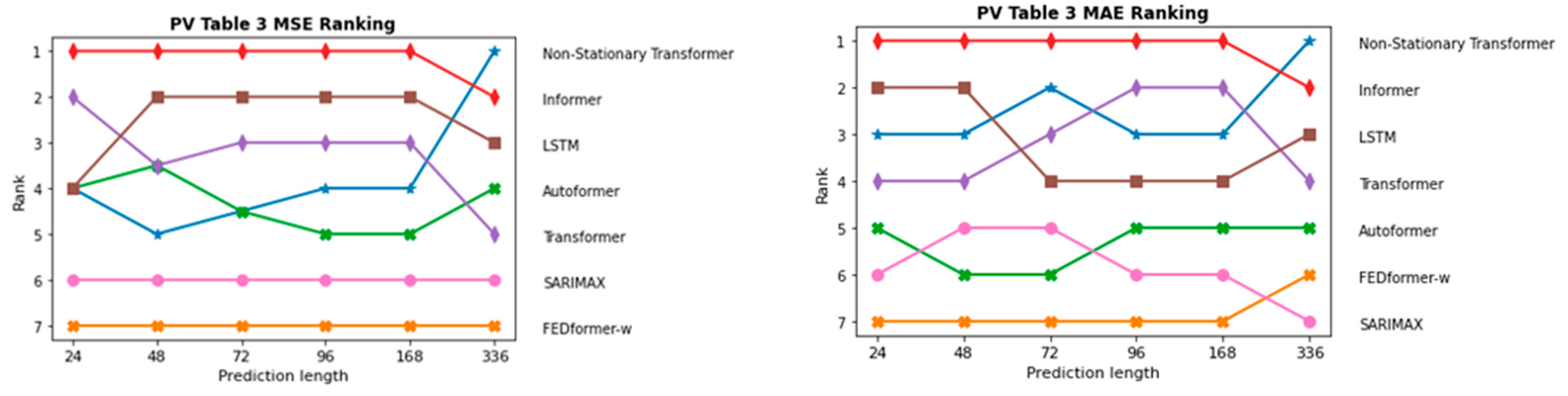
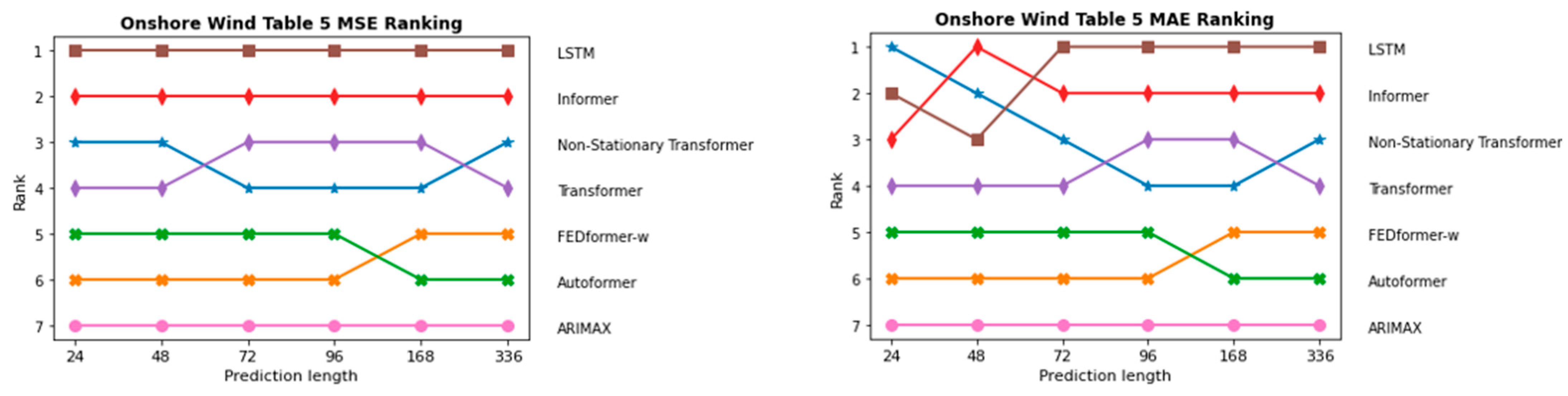
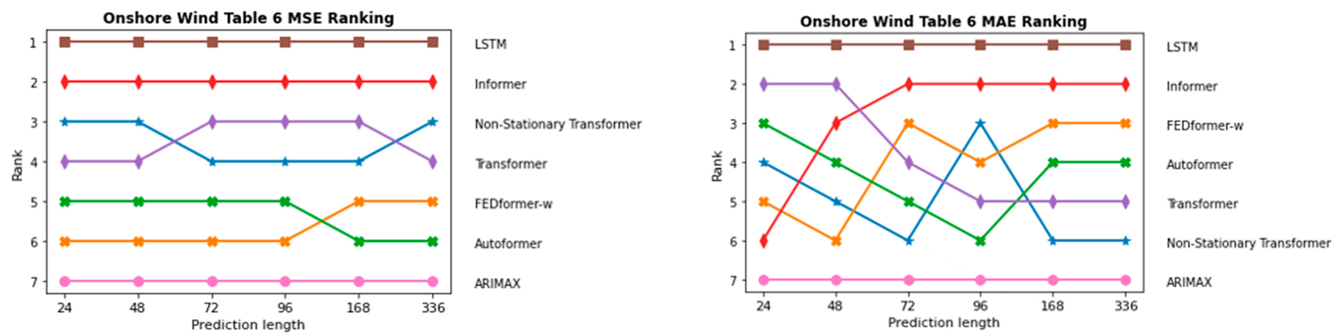
InFigure 19 and Figure 20, the sequence of the order of the individual models in terms of prediction length is depicted once for the two PV forecasting scenarios and in Figure 21 and Figure 22 for the two onshore wind scenarios. As expected, ARIMAX and SARIMAX perform the worst in almost all scenarios. This is because neural networks such as LSTM and Transformer are able to capture more complex patterns in the data as they can model more non-linear relationships. In the initial scenario with all parameters, which is shown in Figure 19, SARIMAX outperforms FEDformer, likely due to data inadequacies, particularly the time component. This is substantiated when examining scenarios for both onshore wind and PV forecasting, where FEDformer significantly improves compared to the initial scenario in terms of the MSE and MAE metrics. When considering the models Autoformer and FEDformer, they are fundamentally based on the idea of decomposing time series into various components or modes. However, as evident from the various rankings provided in Figure 19, Figure 20, Figure 21 and Figure 22, these models consistently lag behind other Transformer models that operate on a different concept. This is surprising, given that in the six benchmarks, these models actually outperform models like Informer or Transformer. Additionally, in the datasets concerning electricity and weather, which belong to the “same” domain as the one being discussed here, these models also exhibit strong performance. It is particularly surprising that FEDformer performs worse in PV energy forecasting, which exhibits a certain periodicity. However, it should be noted that the presented results in FEDformer and Autoformer studies pertain to univariate-to-univariate forecasting and multivariate-to-multivariate forecasting [16,17]. We are considering multivariate-to-univariate forecasting. The Non-Stationary Transformer model undergoes enhanced performance in predicting PV energy, especially with the increase in the forecast horizon compared to other models. It consistently ranks in the top 3 for the forecast horizon of 336, outperforming the base Transformer in terms of the MSE metric. However, it predominantly lags behind the Transformer model in the forecast horizon from 24 to 168 in both PV scenarios and in the forecast horizon from 72 to 168 in both onshore wind scenarios. In the subsequent analysis, the comparison between the Informer model and LSTM model is emphasized, as they predominantly outperform the other models in nearly all areas, especially the LSTM model.

Figure 19.
Comparison of different models in the first PV approach with all parameters via MSE and MAE metrics.
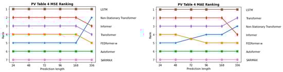
Figure 20.
Comparison of different models in the second PV approach with selected parameters via MSE and MAE metrics.

Figure 21.
Comparison of different models in the first onshore wind approach with all parameters via MSE and MAE metrics.
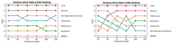
Figure 22.
Comparison of different models in the second onshore wind approach with selected parameters via MSE and MAE metrics.
Table 7 illustrates some patterns when comparing the performance of the LSTM and Informer models across various forecasting scenarios and metrics. In the first scenario, Informer outperforms the LSTM model by an average of 5–8 percent across the forecast horizon of 24 to 336 with respect to the MSE metric. This trend broadly extends to the MAE metric, as well. In the second scenario, the differences favor the LSTM model this time, with approximately a 4 percent improvement in the MSE metric across the forecast horizon of 24–168. The percentage differences in the MAE metric are more variable in this case. The particularly striking aspect is the high percentage value concerning the 336 forecasting range. For the two onshore wind scenarios, there are significantly larger percentage gains for the LSTM model. Particularly surprising are the longer forecast horizons of 168 and 336, as one would expect the Informer model, with its prob sparse self-attention mechanism, to capture longer-term relationships more effectively than the LSTM model. The LSTM model, which typically encounters issues with the vanishing gradient during longer forecasts, does not exhibit this problem in this case. It also became evident during the training process that this problem was not present.
Table 7.
Comparison of performance between LSTM and Informer (− means that Informer performs better; + means that LSTM performs better).
4. Conclusions
This study provides insights into the performance of forecasting models for renewable energies (onshore wind and PV power generation) in Germany. The study examines multivariate-to-univariate prediction, where multiple inputs are used to predict an output variable, such as electricity generated from PV and onshore wind sources, with a focus on Transformer-based models. Our study shows that both Transformer-based models and LSTM can provide considerably more accurate predictions than variants of the classical ARIMA models, but have varying performance in predicting multivariate to univariate outcomes in our application case. A surprising observation is that the LSTM model performs exceptionally well across all forecast horizons and categories and outperforms all used Transformer-based models in most of the forecasting scenarios. This emphasizes the importance of considering the specific nature of the task and data when evaluating a model’s suitability and performance.
In a previous study, the creators of the Non-Stationary Transformer model demonstrated that it outperforms all previously described Transformer-based models across six benchmark datasets, including exchange, ILI, ETTm2, electricity, traffic and weather [15,17]. During this, Non-stationary Transformer proved to be a solid model for the prediction of electricity production from photovoltaics, as well as onshore wind, by using all parameters, especially in the forecast horizon of 336 h. FEDformer can undergo significantly improved performance by using selected higher-correlated weather parameters, while for non-selected parameters in conjunction with the time specification, the model shows significantly worse performance than the other models. In the category of wind power forecasting and PV power forecasting, the Informer model demonstrates superior performance compared to the other Transformer-based models examined in our study. It is noteworthy that the Transformer model performs well in electricity prediction from PV for the selected weather parameters.
In future work, we will investigate forecasts in specific regions, such as a federal state. Additionally, we will select a larger wind farm and use a local weather station to obtain more precise weather data. Furthermore, we will improve the deep learning methods and general methodology for the specific use case of renewable energy production. There are further interesting approaches, like LTSF-Linear [37], that can be analyzed in future investigations. The creators of these models argue that the Transformer models may not be as effective for long-term forecasting tasks as previously thought. This paper introduces a new model called LTSF-Linear, which demonstrates remarkable performance in time series forecasting. What stands out is that this model outperforms several sophisticated Transformer-based models across six benchmark tests for the time period ranging from 96 h to 720 h. This includes well-known models such as FEDformer, Autoformer and Informer. The newest Transformer-based approaches, like Times-Net [38], PatchTST [39] and TSMixer [40], demonstrate, again, better performance across six benchmarks. These models could be utilized for electricity generation through onshore wind and PV and their performance can be compared accordingly.
Author Contributions
Conceptualization, M.J.W. and H.W.; Methodology, M.J.W. and H.W.; Software, M.J.W.; Investigation, M.J.W.; Data curation, M.J.W.; Writing—original draft, M.J.W.; Writing—review & editing, H.W. and M.J.W.; Visualization, M.J.W.; Supervision, H.W.; Project administration, H.W. All authors have read and agreed to the published version of the manuscript.
Funding
This research received no external funding.
Data Availability Statement
Data are contained within the article.
Conflicts of Interest
The authors declare no conflict of interest.
References
- McLennan, M. The Global Risks Report 2022 17th Edition; World Economic Forum: Cologny, Switzerland, 2022; p. 14. Available online: https://www3.weforum.org/docs/WEF_The_Global_Risks_Report_2022.pdf (accessed on 2 July 2023).
- Wöhrle, D. Kohlenstoffkreislauf und Klimawandel. Chem. Unserer Zeit 2020, 55, 112–113. [Google Scholar] [CrossRef]
- Wilke, S. Energiebedingte Emissionen von Klimagasen und Luftschadstoffen. Umweltbundesamt, 6 June 2023. Available online: https://www.umweltbundesamt.de/daten/energie/energiebedingte-emissionen#energiebedingte-kohlendioxid-emissionen-durch-stromerzeugung (accessed on 4 July 2023).
- Aktuelle Fakten zur Photovoltaik in Deutschland. Fraunhofer ISE. p. 48. Available online: https://www.ise.fraunhofer.de/content/dam/ise/de/documents/publications/studies/aktuelle-fakten-zur-photovoltaik-in-deutschland.pdf (accessed on 22 September 2022).
- Umweltbundesamt. Umweltbundesamt. Emissionsbilanz erneuerbarer Energieträger Bestimmung der vermiedenen Emissionen im Jahr 2018. Umweltbundesamt, November 2019; pp. 47–50. Available online: https://www.umweltbundesamt.de/sites/default/files/medien/1410/publikationen/2019-11-07_cc-37-2019_emissionsbilanz-erneuerbarer-energien_2018.pdf (accessed on 2 July 2023).
- Ahmad, T.; Zhang, D.; Huang, C.; Zhang, H.; Dai, N.; Song, Y.; Chen, H. Artificial intelligence in sustainable energy industry: Status Quo, challenges and opportunities. J. Clean. Prod. 2021, 289, 125834. [Google Scholar] [CrossRef]
- Entezari, A.; Aslani, A.; Zahedi, R.; Noorollahi, Y. Artificial intelligence and machine learning in energy systems: A bibliographic perspective. Energy Strategy Rev. 2023, 45, 101017. [Google Scholar] [CrossRef]
- Botterud, A. Forecasting renewable energy for grid operations. In Renewable Energy Integration; Elsevier: Amsterdam, The Netherlands, 2017; pp. 133–143. [Google Scholar] [CrossRef]
- Potter, C.W.; Archambault, A.; Westrick, K. Building a Smarter Smart Grid through Better Renewable Energy Information. Abgerufen von. 1 März 2009. Available online: https://ieeexplore.ieee.org/stamp/stamp.jsp?tp=&arnumber=4840110 (accessed on 18 January 2024).
- Hang, T.; Pinson, P.; Wang, Y.; Weron, R.; Yang, D.; Zareipour, H. Energy Forecasting: A Review and Outlook. 2020. Available online: https://ieeexplore.ieee.org/document/9218967 (accessed on 16 January 2024).
- Chen, X.; Zhang, X.; Dong, M.; Huang, L.; Guo, Y.; He, S. Deep Learning-Based prediction of wind power for multi-turbines in a wind farm. Front. Energy Res. 2021, 9, 723775. [Google Scholar] [CrossRef]
- Gensler, A.; Henze, J.; Sick, B.; Raabe, N. Deep Learning for Solar Power Forecasting—An Approach Using AutoEncoder and LSTM Neural Networks. 1 Oktober 2016. Available online: https://ieeexplore.ieee.org/document/7844673 (accessed on 16 January 2024).
- Bethel, B.J.; Sun, W.; Dong, C.; Wang, D. Forecasting hurricane-forced significant wave heights using a long short-term memory network in the Caribbean Sea. Ocean Sci. 2022, 18, 419–436. [Google Scholar] [CrossRef]
- Gao, C.; Zhou, L.; Zhang, R. A Transformer-Based deep learning model for successful predictions of the 2021 Second-Year La Niña condition. Geophys. Res. Lett. 2023, 50, e2023GL104034. [Google Scholar] [CrossRef]
- Zhou, H.; Zhang, S.; Peng, J.; Zhang, S.; Li, J.; Xiong, H.; Zhang, W. Informer: Beyond Efficient Transformer for Long Sequence Time-Series Forecasting. arXiv 2019. [Google Scholar] [CrossRef]
- Wu, H.; Xu, J.; Wang, J.; Long, M. Autoformer: Decomposition Transformers with Auto-Correlation for Long-Term Series Forecasting. Adv. Neural Inf. Process. Syst. 2021, 34, 22419–22430. [Google Scholar]
- Zhou, T.; Ma, Z.; Wen, Q.; Wang, X.; Sun, L.; Jin, R. FEDformer: Frequency Enhanced Decomposed Transformer for Long-term Series Forecasting. In Proceedings of the International Conference on Machine Learning, PMLR, Baltimore, MD, USA, 17–23 July 2022. [Google Scholar]
- Liu, Y.; Wu, H.; Wang, J.; Long, M. Non-stationary Transformers: Exploring the Stationarity in Time Series Forecasting. Adv. Neural Inf. Process. Syst. 2022, 35, 9881–9893. [Google Scholar]
- Taylor, S.V.; Letham, B. Forecasting at scale. PeerJ Comput. Sci. 2018, 72, 37–45. [Google Scholar] [CrossRef]
- Benti, N.E.; Chaka, M.D.; Semie, A.G. Forecasting Renewable Energy Generation with Machine Learning and Deep Learning: Current Advances and Future Prospects. Sustainability 2023, 15, 7087. [Google Scholar] [CrossRef]
- Hochreiter, S.; Schmidhuber, J. Long Short-Term Memory. 1997. Available online: https://www.bioinf.jku.at/publications/older/2604.pdf (accessed on 7 July 2023).
- Zaremba, W.; Sutskever, I.; Vinyals, O. Recurrent Neural Network Regularization. arXiv 2014, arXiv:1409.2329. [Google Scholar]
- Lai, G.; Chang, W.-C.; Yang, Y.; Liu, H. Modeling Long- and Short-Term Temporal Patterns with Deep Neural Networks. In Proceedings of the 41st International ACM SIGIR Conference on Research & Development in Information Retrieval, Ann Arbor MI USA, 8–12 July 2018. [Google Scholar]
- Dosovitskiy, A.; Beyer, L.; Kolesnikov, A.; Weissenborn, D.; Zhai, X.; Unterthiner, T.; Dehghani, M.; Minderer, M.; Heigold, G.; Gelly, S.; et al. An Image is Worth 16x16 Words: Transformers for Image Recognition at Scale. arXiv 2020, arXiv:2010.11929. [Google Scholar]
- Jamil, S.; Piran, J.; Kwon, O.-J. A Comprehensive Survey of Transformers for Computer Vision. Drones 2023, 7, 287. [Google Scholar] [CrossRef]
- Vaswani, A.; Shazeer, N.; Parmar, N.; Uszkoreit, J.; Jones, L.; Gomez, A.N.; Kaiser, Ł.; Polosukhin, I. Attention Is All You Need. Adv. Neural Inf. Process. Syst. 2017, 30, 5998–6008. [Google Scholar]
- Zhouhaoyi, o.D. GitHub—Zhouhaoyi/Informer2020: The GitHub Repository for the Paper “Informer” Accepted by AAAI 2021. Available online: https://github.com/zhouhaoyi/Informer2020 (accessed on 15 October 2023).
- Lin, Y.; Koprinska, I.; Rana, M. Temporal Convolutional Attention Neural Networks for Time Series Forecasting. In Proceedings of the 2021 International Joint Conference on Neural Networks (IJCNN), Shenzhen, China, 18–22 July 2021; Available online: https://ieeexplore.ieee.org/document/9534351 (accessed on 7 July 2023).
- Wan, R.; Tian, C.; Zhang, W.; Deng, W.-D.; Yang, F. A Multivariate Temporal Convolutional Attention Network for Time-Series Forecasting. Electronics 2022, 11, 1516. [Google Scholar] [CrossRef]
- Qin, Y.; Song, D.; Chen, H.; Cheng, W.; Jiang, G.; Cottrell, G.W. A Dual-Stage Attention-Based Recurrent Neural Network for Time Series Prediction. arXiv 2017, arXiv:1704.02971. [Google Scholar]
- Wang, D.; Chen, C. Spatiotemporal Self-Attention-Based LSTNet for Multivariate Time Series Prediction. Int. J. Intell. Syst. 2023, 2023, 9523230. [Google Scholar] [CrossRef]
- Bundesnetzagentur. SMARD|SMARD—Strommarktdaten, Stromhandel und Stromerzeugung in Deutschland. SMARD. Available online: https://www.smard.de/home (accessed on 16 June 2023).
- Deutscher Wetterdienst Wetter und Klima aus Einer Hand. Climate Data Center. Available online: https://cdc.dwd.de/portal/ (accessed on 24 June 2023).
- Energie-Atlas Bayern—Das Zentrale Informationsportal zur Energiewende in Bayern|Energie-Atlas Bayern. Available online: https://www.energieatlas.bayern.de/ (accessed on 25 January 2024).
- MAZiqing. GitHub—MAZiqing/FEDformer. GitHub. Available online: https://github.com/MAZiqing/FEDformer (accessed on 15 October 2023).
- Thuml. GitHub—thuml/Nonstationary_Transformers: Code Release for ‘Non-Stationary Transformers: Exploring the Stationarity in Time Series Forecasting’ (NeurIPS 2022). GitHub. Available online: https://github.com/thuml/Nonstationary_Transformers (accessed on 15 October 2023).
- Zeng, A.; Chen, M.; Zhang, L.; Xu, Q. Are transformers effective for time series forecasting? arXiv 2022, arXiv:2205.13504. [Google Scholar] [CrossRef]
- Wu, H.; Hu, T.; Liu, Y.; Zhou, H.; Wang, J.; Long, M. TimesNet: Temporal 2D-Variation Modeling for General Time Series Analysis. arXiv 2022, arXiv:2210.02186. [Google Scholar]
- Nie, Y.; Nguyen, N.H.; Sinthong, P.; Kalagnanam, J. A Time Series is Worth 64 Words: Long-term Forecasting with Transformers. arXiv 2022, arXiv:2211.14730. [Google Scholar]
- Chen, S.; Li, C.-L.; Yoder, N.-C.; Arık, S.Ö.; Pfister, T. TSMixer: An All-MLP architecture for time series forecasting. arXiv 2023, arXiv:2303.06053. [Google Scholar]


Disclaimer/Publisher’s Note: The statements, opinions and data contained in all publications are solely those of the individual author(s) and contributor(s) and not of MDPI and/or the editor(s). MDPI and/or the editor(s) disclaim responsibility for any injury to people or property resulting from any ideas, methods, instructions or products referred to in the content. |
© 2024 by the authors. Licensee MDPI, Basel, Switzerland. This article is an open access article distributed under the terms and conditions of the Creative Commons Attribution (CC BY) license (https://creativecommons.org/licenses/by/4.0/).