Article

Detection of Pumping Unit in Complex Scenes by YOLOv7 with Switched Atrous Convolution

School of Petroleum Engineering, China University of Petroleum (East China), Qingdao 266580, China
*
Author to whom correspondence should be addressed.
Energies 2024, 17(4), 835; https://doi.org/10.3390/en17040835
Submission received: 6 January 2024 / Revised: 29 January 2024 / Accepted: 7 February 2024 / Published: 9 February 2024
(This article belongs to the Section H1: Petroleum Engineering)

Abstract

:
The petroleum and natural gas industries exhibit a high dependency on lifting equipment for oil and gas. Any malfunction in these devices can lead to severe economic losses. Therefore, continuous and timely monitoring of the status of pumping equipment is of paramount importance to proactively prevent potential issues. In an effort to enhance this monitoring process, this study delves into multi-source data images at the well site and extends traditional information analysis methods. It introduces an improved YOLOv7 method based on switchable atrous convolution. While the YOLOv7 algorithm achieves a balance between speed and accuracy, its robustness in non-standard environments is suboptimal. To address this limitation, we propose the utilization of a switchable atrous convolution method for enhancement, thereby augmenting the adaptability of the model. Images of pumping units from diverse scenarios are actively collected and utilized to construct training, validation, and test sets. Different models, including YOLOv7SAC, YOLOv7, and YOLOv5-n, undergo testing, and their detection performances are systematically compared in complex environments. Experimental findings demonstrate that YOLOv7SAC consistently attains optimal detection results across various scenes. In conclusion, the study suggests that the combination of the YOLOv7 model with switchable atrous convolution proves effective for detecting pumping unit equipment in complex scenarios. This provides robust theoretical support for the detection and identification of pumping equipment issues under challenging conditions.

1. Introduction

The continuous advancement and implementation of artificial intelligence (AI) technology have brought profound transformations and challenges to society, fostering the intelligent evolution of the oil and gas industry. Within this industry, the pumping unit holds pivotal significance, playing a critical role in the extraction of oil and gas resources. However, owing to the demanding operational conditions and prolonged usage, pumping units are susceptible to wear, potentially resulting in equipment failures and subsequent production losses. Therefore, ensuring the real-time monitoring of the pumping unit’s status for sustained normal operation becomes imperative. Currently, the predominant approach involves establishing data-driven diagnostic models using machine learning techniques based on extensive datasets. This methodology has yielded commendable results, contributing to enhanced recognition accuracy and mitigated production losses attributable to equipment failures. Han and Yue [1], for instance, employed principal component analysis, cluster analysis, and regression analysis to mine and analyze light-rod-load data from aging wells, elucidating the working conditions of oil wells. Lv et al. [2] devised a novel sucker rod pumping system (SRPS) model and introduced an evolutionary support vector machine (SVM) method for SRPS diagnosis, tailored to diverse well diagnostic requirements. Pan et al. [3] introduced a novel decision fusion method rooted in Bayesian theory, utilizing extensive data generated during the production process for unsupervised fault detection in pumping units. Cheng et al. [4] applied transfer learning with AlexNet to extract features from sensor-collected data and employed SVM for identifying working conditions.
The methods mentioned above necessitate the development of diagnostic machine learning models utilizing data, sensors, and other tools. Challenges arise from issues such as data noise and timeliness within massive datasets during the model application, and these issues cannot be overlooked. Moreover, the deployment of sensors and data transmission demand substantial human and material resources. It is crucial to highlight that video monitoring technology ensures the timely availability of image data, and the monitoring deployment process does not require extensive resources, as compared to sensors. Object detection, a technique employed to recognize and locate objects in images or videos, has found widespread applications in various industries, particularly in industrial monitoring. Presently, the algorithm based on deep learning has emerged as the predominant research methodology in this field, showing great promise in intelligent monitoring [5,6]. The algorithms in this field can be broadly categorized into three types: two-stage, one-stage, and vision transformer (ViT). Girshick et al. [7] introduced R-CNN with CNN features for object detection, demonstrating the efficacy of two-stage detectors. In 2015, Redmon et al. [8] proposed the first one-stage detector, YOLOv1, and they have since developed a series of YOLO algorithm frameworks through continuous enhancements. ViT refers to the transformer architecture in natural language processing, which has been extended to the computer vision domain [9] and has yielded positive outcomes on extensive training data. Among various object detection algorithms, the one-stage YOLO series algorithms have exhibited outstanding performance in object detection tasks, especially in industrial applications, where they ensure real-time detection while meeting the requirements for training with limited samples.
Considering the intricacy of the comprehensive balance model and the precision demands of application scenarios, we enhanced the detection of oil pumping machines using the YOLOv7 algorithm framework [10] and conducted evaluations on a practical oil-pumping-machine dataset. YOLOv7, being a one-stage object detection algorithm, maintains high accuracy while ensuring rapid response times. To enhance the algorithm’s adaptability to complex environments, we employed the improved YOLOv7 algorithm with switchable atrous convolution (referred to as YOLOv7SAC) for the detection of oil-pumping-machine equipment. This approach facilitates the real-time monitoring of oil-pumping-machine statuses, enables the prompt detection of equipment failures, and mitigates production losses. Conventional detection methods necessitate manual intervention, resulting in inefficiency. In contrast, the utilization of object detection algorithms allows for automated detection, enhancing monitoring efficiency and accuracy.
The method proposed in this paper employs real oil-pumping-machine image datasets for training and employs transfer learning to train the YOLOv7SAC algorithm on the annotated dataset. Transfer learning is a technology that reduces training time, diminishes the demand for computing resources, and enhances the model’s generalizability. Through transfer learning, we leverage models trained on large-scale datasets to transfer their knowledge to target tasks, thereby improving model performance in new tasks. We initialized the YOLOv7SAC model using a pre-trained model on the COCO dataset [11] and fine-tuned it on the annotated dataset. The oil-pumping-machine image datasets used for training and testing are derived from real oil fields, encompassing various types of oil-pumping-machine devices in diverse scenarios. The annotated dataset precisely delineates the position of oil-pumping-machine equipment in the image, and transfer learning is then applied to train the YOLOv7SAC algorithm on this annotated dataset.
This study contributes via the following aspects: (1) It introduces intelligent technology for well-site recognition monitoring, addressing the current challenges of time-consuming and labor-intensive well-site surveillance. This is conducive to facilitating future unmanned supervision of well-site development. (2) To address the challenge of detecting high-density pumping units in complex well-site environments using YOLOv7, improvements are made by incorporating switchable atrous convolutions, resulting in enhanced accuracy. (3) The proposed method is validated through real-world well-site scenarios, confirming the effectiveness of the approach.

2. Related Work

Object detection stands as a pivotal domain in computer vision, where various machine learning (ML) and deep learning (DL) models have been employed to enhance performance in object detection and related tasks. Initially, two-stage object detectors demonstrated excellent detection performance and found widespread applicability. However, recent advancements in one-stage object detection and bottom-up algorithms have underscored their improved performance and stability, positioning them as competitive counterparts to most two-stage object detectors. Furthermore, the introduction of YOLOv5 has seen its widespread adoption for object detection and recognition across diverse backgrounds, showcasing notable performance compared to corresponding two-stage detectors. This highlights the YOLO algorithm’s excellent compatibility with new modules. In laying the groundwork for the network model of the YOLOv7 algorithm, this section introduces fundamental concepts and architecture. It also explores incremental optimizations implemented in different YOLO versions compared to their predecessors within the YOLO algorithm framework.
YOLOv1 [8] redefined the object detection problem as a regression problem instead of a classification problem. The efficacy of convolutional neural networks (CNNs) in extracting features from a visual input is attributed to the efficient propagation of low-level features from the initial convolutional layer to subsequent layers in a deep CNN. The challenge resides in the precise identification of multiple objects and the determination of their exact spatial locations within a singular visual input. Two pivotal attributes of CNNs, namely parameter sharing and the utilization of multiple filters, adeptly tackle the intricacies associated with object detection. The CNN predicts all object boundary boxes and class probabilities in the image, utilizing bounding boxes to recognize objects and their positions in a single image. YOLO’s straightforward structure, coupled with its innovative full-image, one-shot regression, enhances its speed compared to existing object detectors, enabling real-time performance. However, despite YOLO’s faster performance relative to conventional object detectors, it exhibits larger location errors compared to other advanced two-stage methods. This limitation arises from its ability to detect, at most, two objects of the same class within a grid cell, thereby restricting its capability to predict nearby objects. Additionally, it poorly adapts to objects with aspect ratios not encountered during training, and due to the presence of down-sampling layers, it can only learn from coarse object features.
YOLOv2 [12] introduced a novel hierarchical approach building upon YOLOv1, merging classification and detection tasks, significantly enhancing model scalability concerning the number of classes. To maintain consistency in the weight matrix distribution across different levels and mitigate the issue of internal covariate shift, batch normalization was incorporated, normalizing the output from each hidden layer. The removal of fully connected layers increased the flexibility of the model prediction dimensionality, facilitating multi-scalable training and improving the detection resolution. In this iteration, anchor was employed for predicting boundary boxes, utilizing a set of predefined anchor prototypes with matching object shapes. Multiple anchors were assigned to each grid cell, predicting the coordinates and categories of each anchor. The network’s output size is directly proportional to the number of anchors in each grid cell. YOLOv2 incorporated clustering analysis to select optimal anchors, enhancing the network’s ability to predict more accurate boundary boxes. During training, k-means clustering was performed on the boundary boxes to identify suitable anchors, striking a balance between recall rate and model complexity.
YOLOv3 [13] embraced the concept of feature pyramid networks (FPNs) [14], integrating residual blocks, skip connections, and up-sampling into the network structure. This connection of down-sampled feature maps to up-sampled feature maps at different locations facilitated the extraction of fine-grained features, which is particularly beneficial for detecting small objects of varying dimensions. Different feature maps of 52 × 52, 13 × 13, and 26 × 26 were employed to detect large, medium, and small objects, separately.
YOLOv4 [15] enhances the backbone network by transforming Darknet53 into CSP Darknet53 based on YOLOv3. CSP Darknet53 splits into two branches after the base layer, eventually merging the two to achieve richer gradient combinations with a smaller computational cost. Spatial pyramid pooling (SPP) [16] is introduced behind the backbone network in YOLOv4 to significantly increase the receptive fields, capturing more prominent contextual features. To enhance model robustness against perturbations, image adversarial attacks are employed to generate deceptive training data with a falsely labeled ground truth. These deceptive data were retained to enable the model to correctly detect objects. YOLOv4 utilizes genetic algorithms for hyperparameter optimization. A genetic algorithm is employed in the initial 10% of the training period to find the best hyperparameters for training. Additionally, a cosine annealing scheduler is employed to adjust the learning rate throughout the entire training process. The algorithm structure gradually reduces the learning rate at the beginning of training, rapidly reduces it at the midpoint, and slightly reduces it towards the end, enabling adaptive learning habits based on the network structure.
In YOLOv5, the network structure is streamlined by introducing two parameters: model depth and the number of convolutional kernels. Additionally, it incorporates two data augmentation methods, scaling and color space adjustment, building upon the mosaic data augmentation used in YOLOv4. A focus layer is added in front of the backbone network in YOLOv5 to more fully extract features without information loss.
YOLOv7 introduces model reparameterization into the framework. It constructs a series of structures for training and equivalently transforms their parameters into another set of inference parameters. This equivalence allows conversion of the initial series of structures into another, helping the model optimize its performance based on specific task requirements and enhance generalization. Furthermore, YOLOv7 introduces proportional scaling to address the accuracy–speed trade-off in different scenarios, utilizing distinct model extension strategies for scaling up.

3. Proposed Method

This study delves into the exploration based on YOLOv7, a model that demonstrates significant advantages in the domain of object detection. Contrasted with YOLOv5, YOLOv7 exhibits improvements in both precision and speed in object detection. Testing on the MS COCO dataset indicates that YOLOv7-X reduces parameters by 22% and computations by 8% compared to YOLOv5-X, while increasing the average precision (AP) by 2.2%. Renowned for its speed and efficiency, YOLOv7 achieves more accurate detection of small and occluded targets through innovative designs such as multi-scale fusion and path integration. Its end-to-end training strategy and adaptability to various target sizes make the model perform exceptionally well in complex scenarios. However, YOLOv7’s performance may decrease when dealing with dense targets. Additionally, in scenarios with complex backgrounds and low contrast, YOLOv7’s detection accuracy may be compromised. This study, building upon the strengths of YOLOv7, addresses its shortcomings with targeted improvements, further enhancing the accuracy and stability of the object detection model in the context of oilfield development. The YOLOv7SAC network structure designed in this study is shown in Figure 1.

3.1. Network Structure

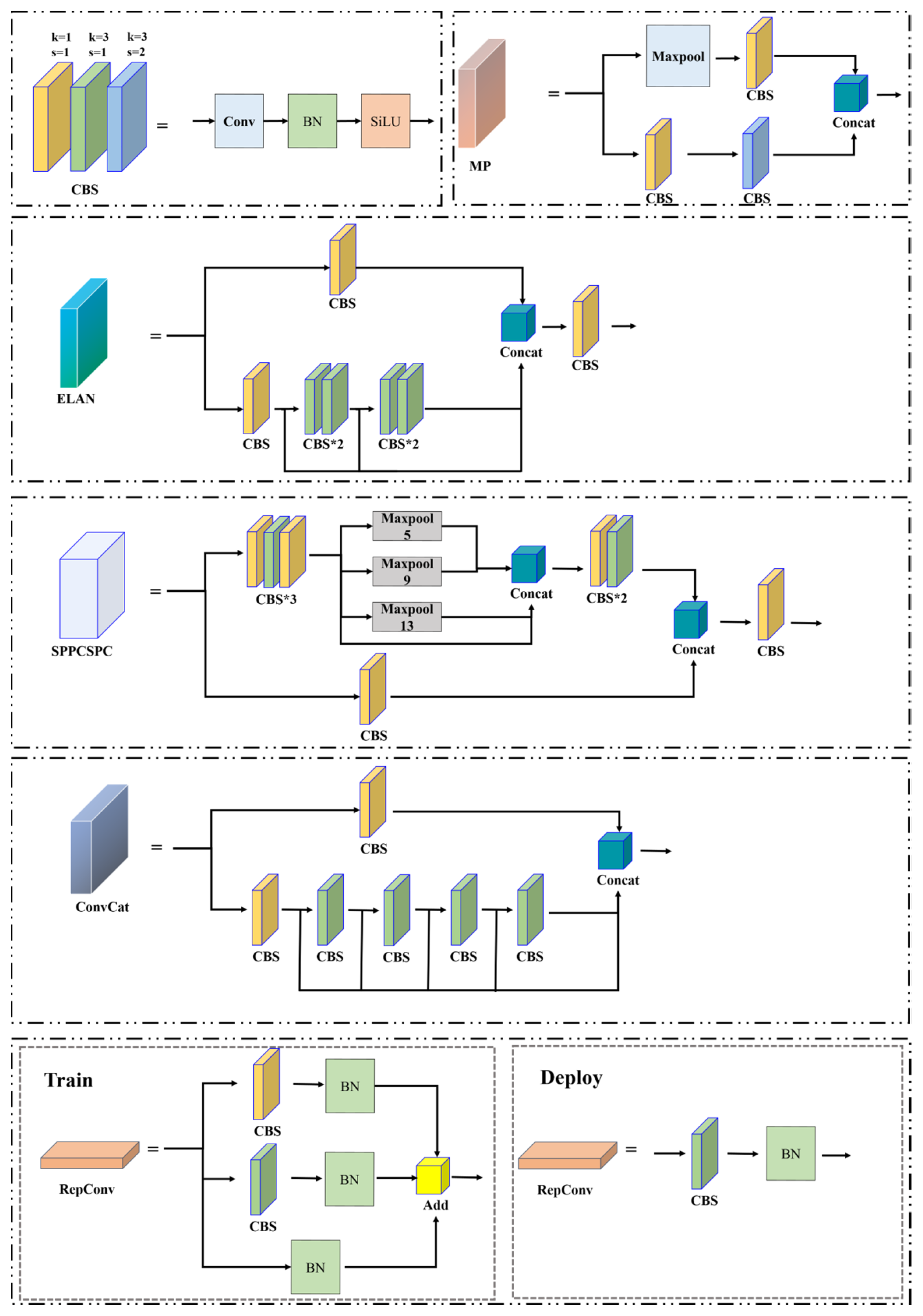
According to the diagram, the network structure of YOLOv7SAC is composed of four parts: the input network, backbone network, neck network, and head network. The image is first processed by the input network structure of YOLOv7SAC, and the image size is resized to 640 × 640 × 3 before being input into the backbone network. The CBS module, efficient layer aggregation network (ELAN), and MP1 module alternately down-sample the feature map to half of the original scale, while the output channel number becomes twice the input channel number. The structure of each module in the YOLOv7SAC network structure is shown in Figure 2. The CBS module performs convolution on the input feature map, then uses batch normalization to reduce the problem of internal covariate shift. Finally, it uses an activation function to introduce non-linear features, where the activation function uses the same SiLU activation function [17] as YOLOv5, which is obtained by the following formula:
S i L U ( x ) = x 1 + e x
where SiLU(x) is the output value of the activation function and x is the input value of the function.
There are three types of CBS modules in the structure, each with different convolution kernels (k) and strides (s). The yellow CBS module is a 1 × 1 convolution with a stride of 1, and its main function is to change the channel number; the green CBS module is a 3 × 3 convolution with a stride of 1, and its main function is to extract features; the blue CBS module is a 3 × 3 convolution with a stride of 2, and its main function is down-sampling.
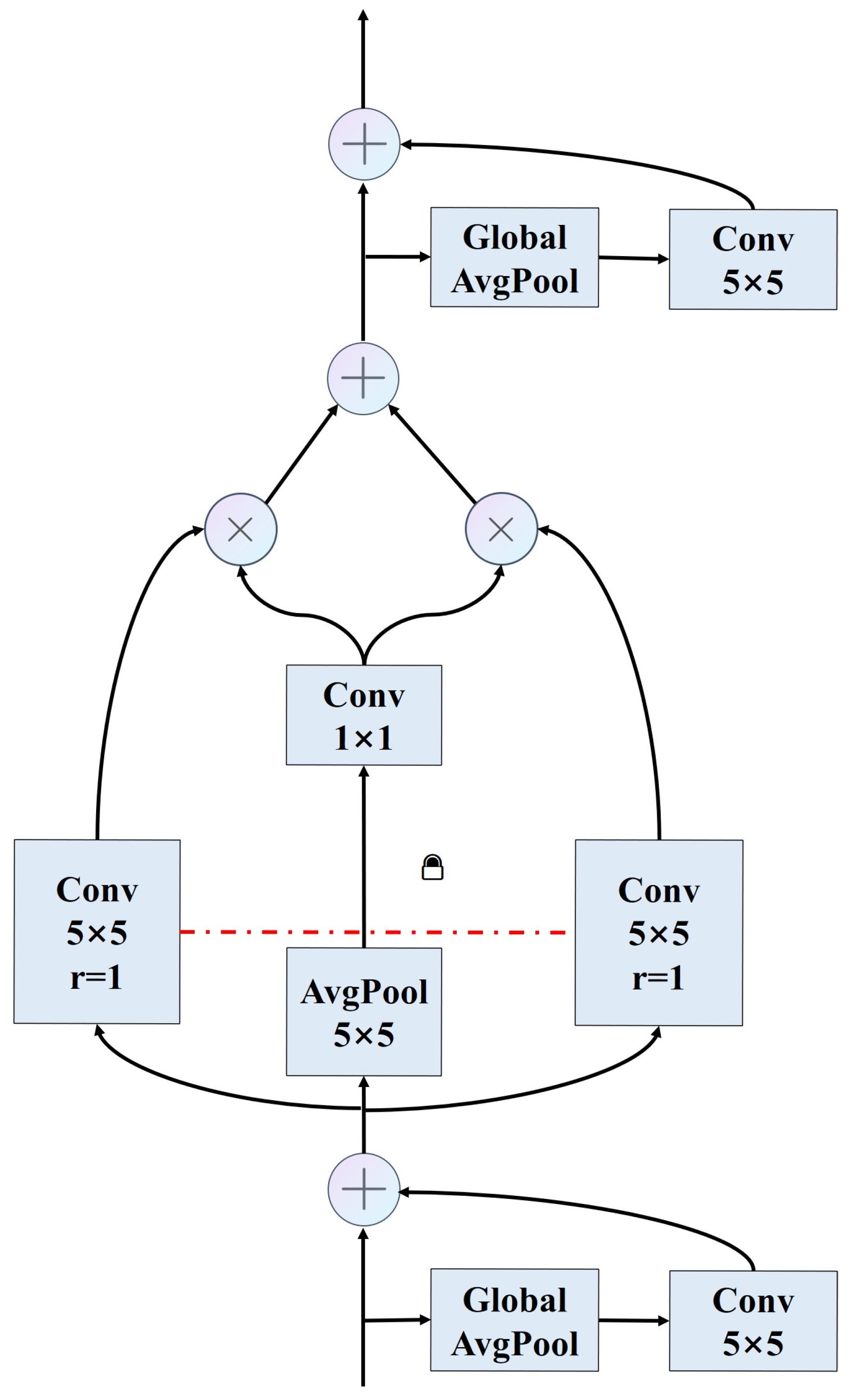
Atrous convolution is an effective technique for increasing the receptive field of convolution kernels in convolutional layers. It can enlarge the size of convolution kernels without increasing the number of parameters or computational complexity. Switchable atrous convolution (SAC) [18] has designed an efficient transformation mechanism that can transform standard convolution into conditional convolution, i.e., dynamically adjusting the convolution kernel, width, or depth of convolutional operations. Through the spatial switch function, this technology can make each feature mapping area have different switch functions to control the output of SAC, which can greatly improve the performance of the detector. The transformation formula is as follows:
C o n v ( x , w , 1 ) S ( x ) · C o n v ( x , w , 1 ) + ( 1 S ( x ) ) · C o n v ( x , w + Δ w , r )
where x is the input; w is the weight; r is the void ratio of the void convolution, which is the trainable weight; and S(x) is the switching function, which consists of a 5 × 5 average pooling layer and a 1 × 1 convolution layer. The SAC structure is shown in Figure 3.
In order to continually enhance the learning capabilities of the network without disrupting the existing gradient pathways, YOLOv7SAC introduces the efficient layer aggregation network (ELAN). The ELAN structure consists of different CBS convolutional modules. Group convolution is employed to expand the channels and cardinality of the computation block, ensuring that the number of channels in each group feature map is the same as in the original architecture. Ultimately, the number of channels exported from the ELAN module is twice that of the input.
The upper branch of the MP1 module reduces the size of the feature map by half through max pooling, and the channel is halved through the CBS convolution module; the lower branch first cuts the channel in half through the CBS convolution module, and then reduces the size of the feature map by half through the CBS convolution module with a 3 × 3 kernel and a stride of 2; then, the whole branches are fused. Eventually, the obtained output feature map has a length and width that is half of the input, with equal input and output channels. Similarly, the MP2 module is similar to the MP1 module, except that the output channels of the output feature map are twice the input feature map.
In order to expand the receptive field without losing resolution, the MP1-S module and ELAN-S module based on the SAC convolution model were designed at the end of the backbone network. The difference from the previous modules is that the normal convolution in the 3 × 3 CBS convolution of the ELAN and MP1 modules is replaced by switchable atrous convolution, achieving a smooth switching between different dilation rates for convolutional calculations. Two global contextual modules in the structure add image-level information to the features.
On the basis of the three outputs in the backbone network, the neck network adopts the same Pa-FPN [14,19] structure as YOLOv4 and YOLOv5 to continue outputting three different-sized feature maps. The neck network is composed of an SPPCSC module, a sequence of CBS modules, an MP module, and a ConvCat module. For the feature map with a 32× down-sampling output from the end of the backbone network, it is first processed by the SPPCSC module. After being processed by the SPPCSC module, the channel number of the feature map is reduced from 1024 to 512. The following process is the same as for YOLOv5, following the top-down route, and then integrating with 16× and 8× down-sampling feature maps in turn to obtain three feature maps of sizes 20 × 20 × 512, 40 × 40 × 256, and 80 × 80 × 128; then, the down-top route is followed to integrate with the 20 × 20 × 512 and 40 × 40 × 256 feature maps.
In the neck network, the ConvCat module is similar in structure to the ELAN module, but the number of ConvCat is increased from 4 to 6. Unlike the SPPF used in YOLOv5, YOLOv7SAC uses the better-performing SPPCPC module to increase the network’s receptive field. First, a 20 × 20 × 512 input feature map is obtained and undergoes three CBS convolution operations, followed by three max pooling operations with kernel sizes of 5, 9, and 13, where the application of padding is adaptable to various kernel sizes. Finally, the result is combined with data from a 1 × 1 CBS convolution operation only, without pooling, to obtain a feature map with a size of 20 × 20 × 512. The SPPCPC module can obtain adaptive scale object information while keeping the size of the feature map constant.
For the three differently sized feature maps output by the neck network, YOLOv7SAC designs the structured re-parameterized convolution using the RepConv structure [20] without direct connection, which increases training time but greatly improves inference performance [21]. In the training process, the entire module is divided into multiple identical or different module branches. In addition, 3 × 3 CBS convolution with batch normalization, 1 × 1 CBS convolution with batch normalization, and batch normalization layers when the input and output channels are the same are added to obtain the training model. In the inference process, the three parts are re-parameterized and their parameters are equivalently converted to another set of parameters using a 3 × 3 CBS convolutional module output. Then, the multi-branch training model is transformed into a high-speed single-branch inference model. The deployed model retains the high accuracy and other excellent characteristics of the multi-branch model while maintaining efficiency. It achieves a good balance between speed and accuracy, thereby improving network performance.
After adjusting the final number of output channels in the RepConv module, 1 × 1 three-layer convolution is used to perform object, class, and bounding box prediction tasks for object detection, obtaining the final detection results.

3.2. Training Strategy

Regular parameter weights accumulate the gradient throughout the entire training process. Meanwhile, using the EMA (exponential moving average) parameter weights is equivalent to using a weighted average of the gradients during training, with small initial weights for the gradients, computing the weighted average of all previous data points, and the weight follows an exponential decay. Since the beginning of training is often unstable, the gradients obtained at the beginning should be given lower weights, and using EMA during model training can improve test metrics and increase the robustness of the model. The formula for calculating EMA is as follows:
v t = β · v t 1 + ( 1 β ) · θ t
where v t represents the shadow weights at time t ( v 0 = 0 ), β is the weighted value, and θ t is the model weights at time t.
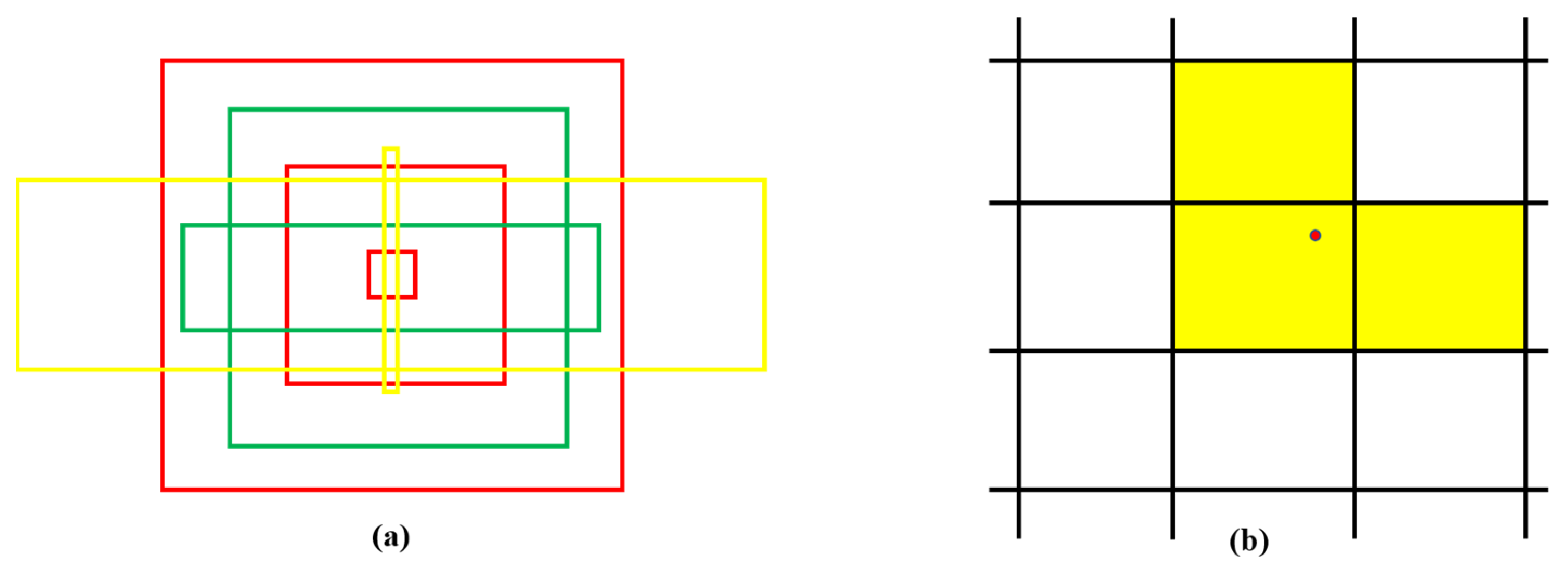
In terms of label assignment, first match the real box with the anchor box aspect ratio and increase the positive sample number on the basis of the nearest center. If the aspect ratio falls within a certain range, as shown in Figure 4a, the anchor box is the red square in the middle, with another red square inside and outside. The ratio inside to outside is 1/4 and 4, respectively, with a range of four times. As long as the width and height of the real box fall within the range of the inside and outside, it is considered a match and the anchor box can be used to predict the real box. The green box in the figure indicates a successful match, and the yellow box indicates a failure. To further increase the number of positive samples, the two grids closest to the center of the real box also make predictions for the real box, as shown in Figure 4b.
After finding the positive samples for predicting the real box, they are further processed using OTA [22] label matching to select the most suitable anchor boxes. The general idea is to first restore the normalized real box to the real size and coordinates, and then match the preliminarily selected anchor boxes with the predicted boxes to find the predicted boxes corresponding to these anchor boxes. Since the predicted boxes are offset relative to the anchor boxes, their centers and widths/heights are decoded. Each real box’s IoU is calculated with all preliminarily selected positive samples, and the sum of the calculation results is rounded to obtain a value k, which is the number of positive sample anchor boxes to be selected for this real box. One real box can correspond to multiple positive samples, and one positive sample anchor box can only correspond to one real box. The target class loss is calculated for each real box and all preliminarily selected positive samples, and the IoU loss is then added to the target class loss to obtain the total loss. The total loss calculation result of the predicted boxes corresponding to all preliminarily selected positive samples for one real box is sorted, and the minimum k values are taken. The anchor boxes corresponding to these values are the final positive samples. If a positive sample corresponds to multiple ground truth boxes, the positive sample is extracted, and the total loss value between the positive sample and the multiple ground truth boxes is computed. The minimum total loss value is then found, and the positive sample is assigned to predict that ground truth box with the smallest total loss.
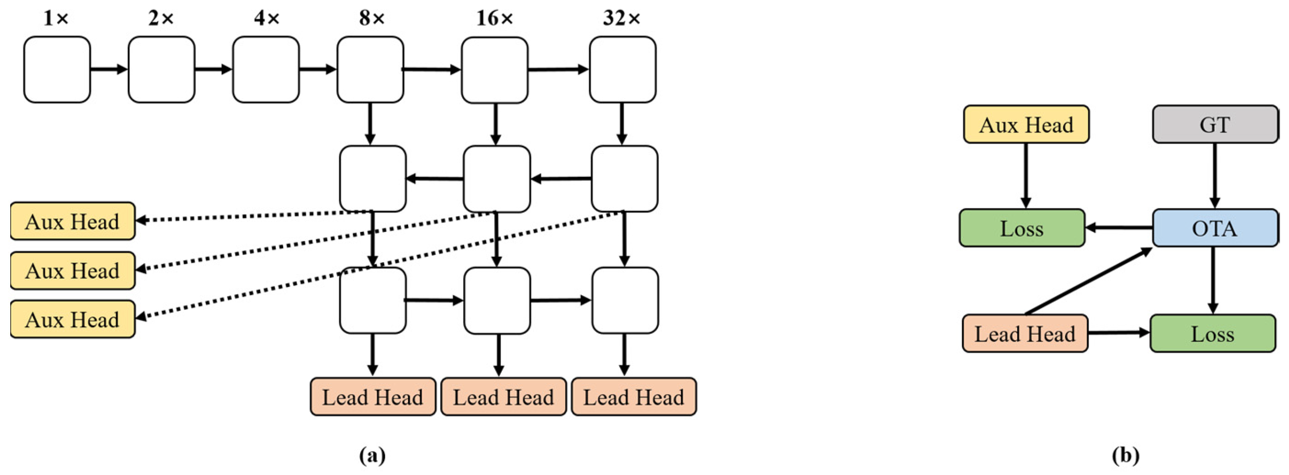
During the training process, YOLOv7SAC utilizes a deep supervision technique, where the shallow features are extracted from the header as the auxiliary header, and the deep features of the final output of the network are used as the guiding header, as shown in Figure 5a. The losses from the auxiliary and lead heads are fused, equivalent to performing a model ensemble operation at the network’s high level, which enhances the overall model performance. When computing the loss, the lead head calculates loss independently, while the auxiliary head takes the positive samples matched by the lead head as its own positive samples and calculates loss. Finally, the losses from both heads are added according to different proportions, as shown in Figure 5b.

3.3. Loss Function

The loss function is composed of multiple components, each corresponding to different differences between the model’s predicted results and the annotations. During training, the model adjusts its parameters based on the value of the loss function, aiming to continually reduce the loss function value, thereby improving the model’s accuracy and generalizability. Therefore, the loss function plays an important role in object detection algorithms, directly impacting the training and detection performance of the model.
After two rounds of filtering based on label assignment, the positive samples are obtained, and the loss is computed for each positive sample and its corresponding ground truth box (GT). YOLOv7SAC’s loss function calculation is similar to YOLOv5’s, consisting of three components, namely object confidence loss, class confidence loss, and bounding box regression loss. The object and class confidence loss functions are both calculated using BCE loss, whose formulas are as follows:
L = 1 N i = 1 N [ y i log ( y i ) + ( 1 y i ) log ( 1 y i ) ]
where L is the BCE loss value, N is the total number of samples, and y i is the category of the first sample.
CIoU Loss [23] is used to calculate the loss of coordinate regression. Compared with previous algorithms, the loss function increases the loss of the detection frame scale and the loss of length and width, so that the prediction frame will be more in line with the real frame. The calculation formula is as follows:
α = ν ( 1 I o U ) + ν
ν = 4 π 2 ( arctan w g t h g t arctan w h ) 2
L = 1 I o U + ( ρ 2 ( b , b g t ) c 2 + α ν )
where L is the CIoU loss value, I o U represents the ratio of the areas where the real frame intersects and merges with the prediction frame, c represents the Euclidean distance between the center points of the prediction frame and the real frame, and w ,   h ,   w g t ,   h g t represent the width and height of the prediction frame and the real frame, respectively, as shown in Figure 6.
The three loss functions are weighted and summed according to a certain weight, and the specific calculation formula is as follows:
L = λ 1 L 1 + λ 2 L 2 + λ 3 L 3
where L is the total loss function, L 1 , L 2 , and L 3 represent the target confidence loss, category confidence loss and coordinate regression loss, respectively, and λ 1 , λ 2 , λ 3 are the weight coefficients taken as λ 1 = 0.1 ,   λ 2 = 0.125 ,   λ 3 = 0.05 here, respectively. The loss function is a function used to measure the difference between the model’s predicted results and the actual labels. During the training process, by continuously adjusting the model parameters, the model can more accurately predict the location and category of the targets, thereby improving the accuracy and generalizability of the model.

4. Application

4.1. Model Construction

A total of over 1000 images of pumping units were collected from actual oil field sites with multiple scenarios and angles for model construction. The construction process of the pumping unit detection model consists of two stages: training and testing. In the training stage, the YOLOv7SAC neural network was trained using the training set. After obtaining the model weights during the training process, evaluation indicators were validated on the validation set. The best-weighted model was selected as the pumping unit detection model upon completion of training. During the testing stage, the testing set data were used to run the detection model and evaluate the model applied to the testing set to ensure the model’s applicability and generalization. The model construction and validation processes are shown in Figure 7, where the neural network model’s final output is the confidence of the detected box of the identified pumping unit and the corresponding class. In the application process, actual video data or image data are utilized as the inputs for the model, aiming to achieve accurate monitoring of pumping units and extract crucial spatial information. With the aid of advanced deep learning technology, particularly the improved YOLOv7 object detection network, efficient detection of pumping units has been successfully accomplished. The model output encompasses precise spatial information such as the position and dimensions of the pumping units, providing real-time and accurate data support for well-site operations.

4.2. Model Evaluation

In this study, metrics such as precision, recall, mean average precision (mAP), and F1 score were employed for the objective assessment of the model’s performance. Precision, a commonly used evaluation metric, is calculated as the number of correctly identified targets divided by the total number of detected targets. Generally, higher precision indicates better detection performance. However, elevated precision does not always signify overall effectiveness. Therefore, additional metrics such as mean average precision, recall, and F1 score were introduced for a comprehensive evaluation. The formulas for precision, recall, mean average precision, and F1 score are as follows:
P = T P T P + F P × 100 %
R = T P T P + F N
m A P = 1 n i = 1 n 0 1 P i ( r ) d r
F 1 = 2 P R P + R
where P represents precision, R denotes recall, mAP stands for mean average precision, and F1 signifies the F1 score; the following definitions apply: TP (true positives) signifies the number of correctly detected pumping unit objects; FP (false positives) indicates the number of non-pumping unit objects incorrectly identified as pumping units; and FN (false negatives) represents the number of pumping units that have not been found.

4.3. Results and Discussion

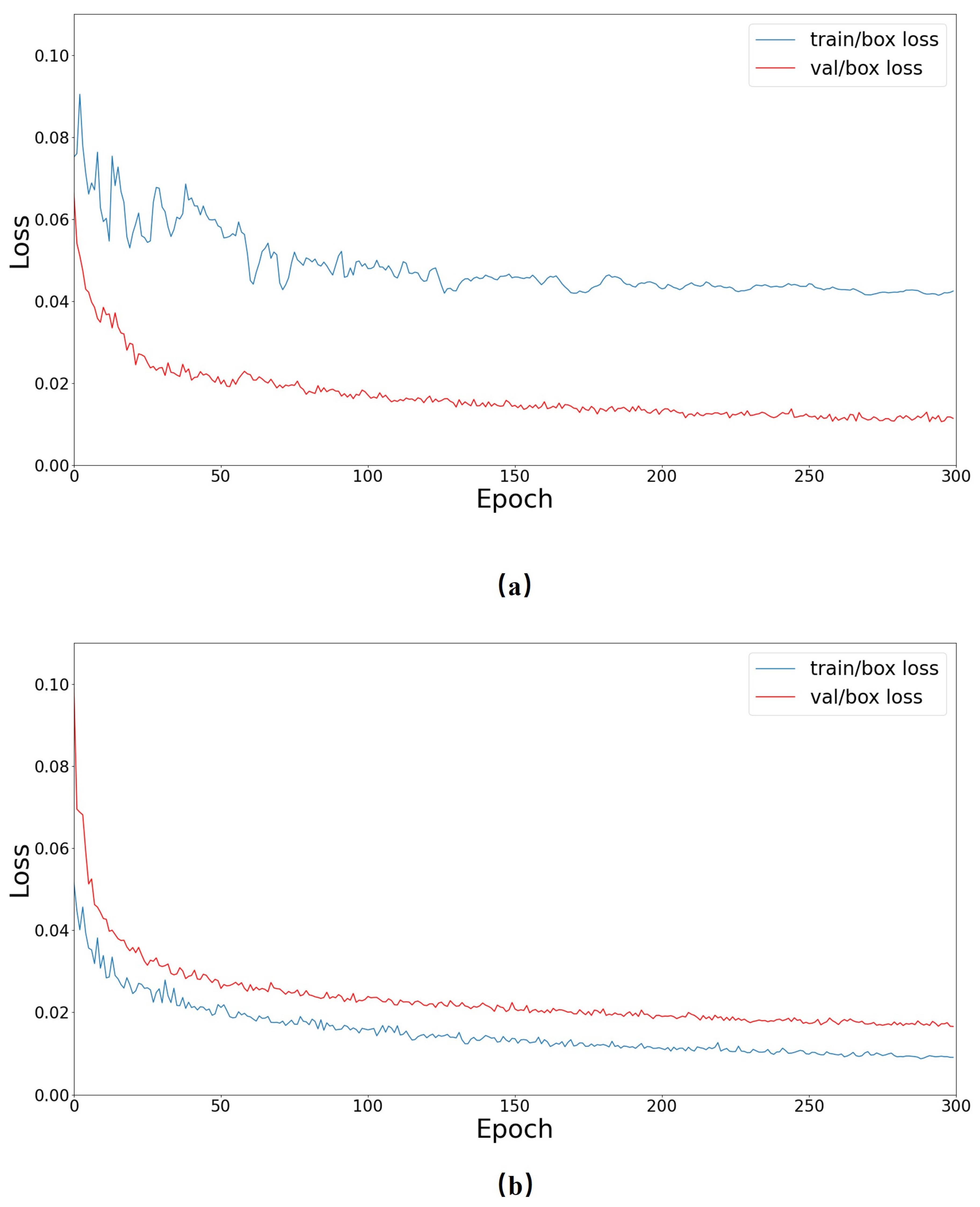
On the basis of the original dataset and the enhanced YOLOv7 network, the YOLOv7SAC model for the target detection of pumping units is established. The training and validation loss fitting curves of the YOLOv7SAC model before and after improvement are shown in Figure 8, in which the horizontal coordinates and vertical coordinates represent the iteration times and the loss function, respectively. The training and validation losses of YOLOv7SAC rapidly decreased in the first 100 epochs, with the validation loss values being higher than the training loss values. Subsequently, in the following 100 to 250 epochs, the losses gradually decreased, reaching stability at around 250 epochs. The loss curves for training and validation converged without overfitting during the training. Therefore, this study determined that the model is suitable for pumping unit detection after 300 epochs.
The value of training loss of the YOLOv7 model converges to 0.012, and that of validation loss converges to 0.017. After improvement, the value of training loss of the YOLOv7SAC model converges to 0.009, and that of validation loss converges to 0.016. Compared with the loss value before improvement, it can be seen that the convergence speed is faster and the detection effect is better.
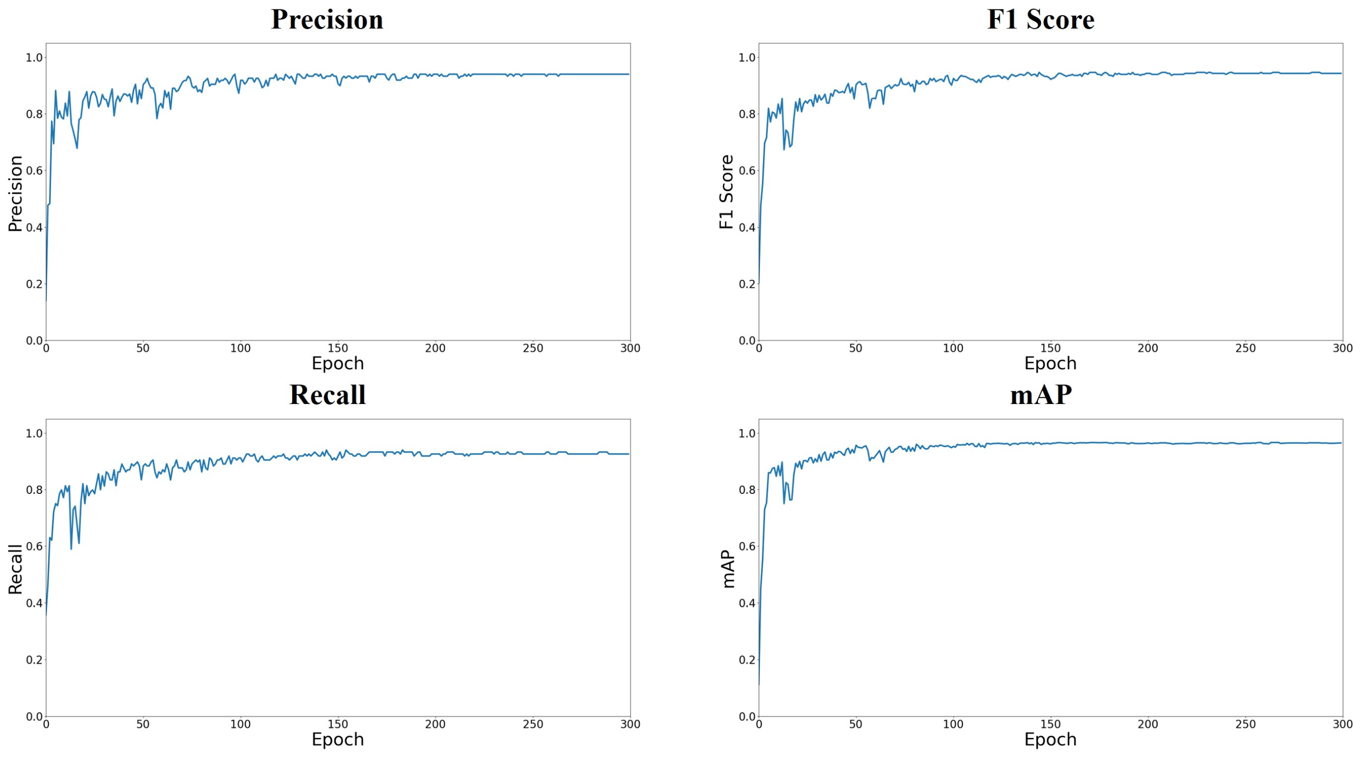
The improved YOLOv7SAC model is compared with YOLOv7 and YOLOv5-n to verify its accuracy and effectiveness. The models all use the MS COCO dataset as the pre-training dataset, the basic weights and parameters of the pre-training model are established, and then the pumping unit image is used as the training dataset. The precision, recall, mean average precision, and F1 score mentioned above are used as the evaluation indexes of different models, and the changes in each index of YOLOv7SAC in the training process are shown in Figure 9. The training results of each algorithm are shown in Table 1. From the table, it can be seen that the accuracy of YOLOv7SAC is improved by 3.76% compared with YOLOv7 and by 8.05% compared with YOLOv5-n; in terms of recall rate, YOLOv7SAC increased by 0.79% compared with YOLOv7 and by 12.20% compared with YOLOv5-n; in terms of F1 score, YOLOv7SAC increased by 2.26% compared with YOLOv7 and by 10.14% compared with YOLOv5-n; in terms of mAP, YOLOv7SAC is 0.73% higher than YOLOv7 and 6.59% higher than YOLOv5-n.
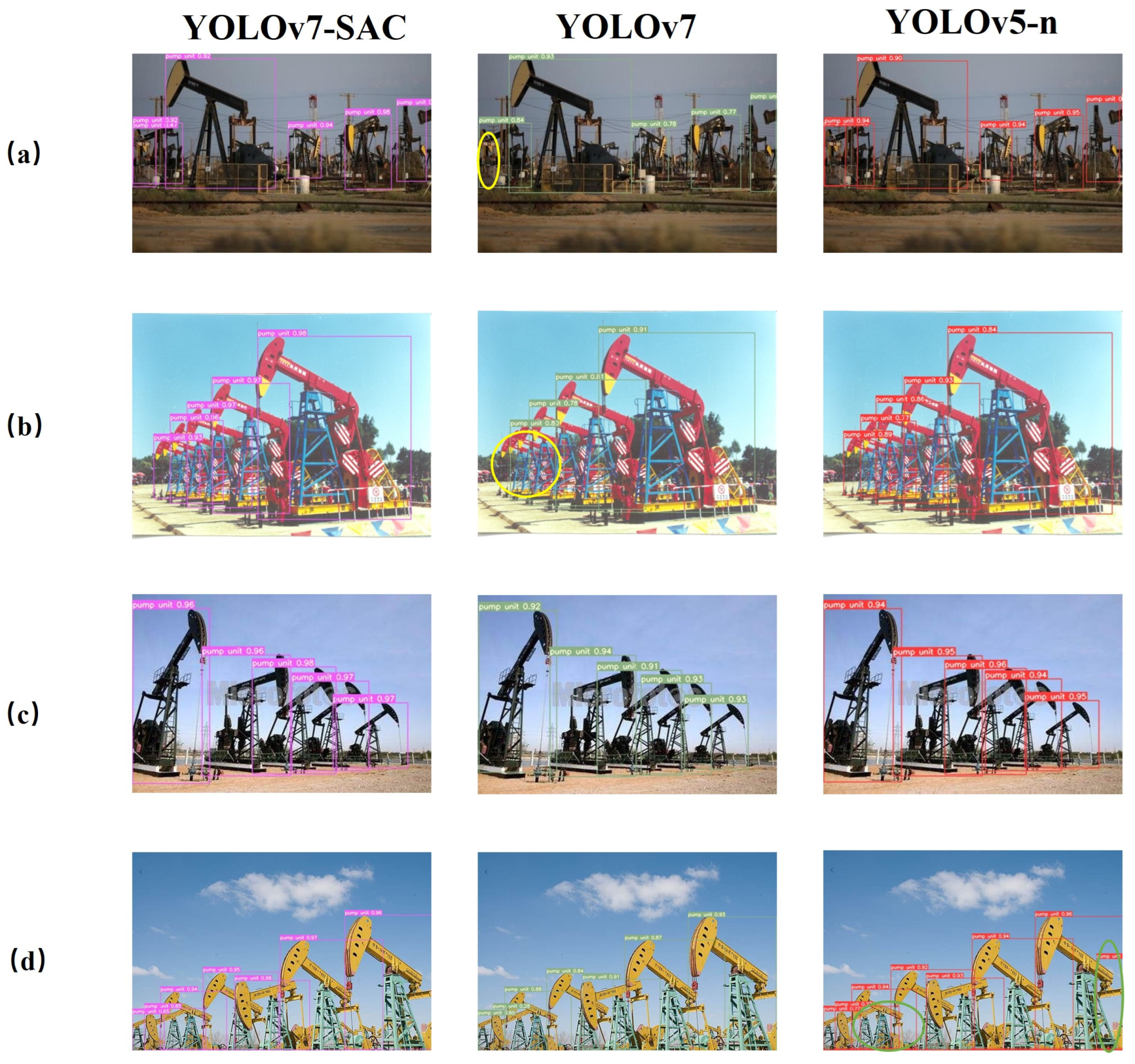
In order to examine the generalizability of different models for pumping unit image detection, the optimal network weights trained by each model are used to detect the data in the test set. In practical application, the detection of a pumping unit needs to ensure the correctness of certain detection, reduce the extra operation brought by the wrong detection, and affect the economic effect. Therefore, the confidence threshold of the detection results is set to 0.4, and the detection effect of each model is shown in Figure 10. The figure shows the detection effect of four scenes; (a) represents the detection effect of pumping units at different scales, (b) represents the scene in which multiple pumping units overlap and block each other, (c) represents the scene in which the pumping units are observed from different angles, and (d) represents the scene in which the pumping unit image does not completely show the overall outline of the pumping unit. Here, the yellow circle represents the pumping unit that has a missed detection, and the green circle represents that the non-pumping unit object is wrongly detected as a pumping unit. From the detection of these scenes, it can be seen that YOLOv7 SAC can detect more pumping unit targets while ensuring the correct detection rate, compared with the YOLOv5-n and YOLOv7 algorithms.
The detection results of on-site image tests in the previous sections are presented in Table 2. The results obtained on the V100 computing graphics card indicate that YOLOv5-n exhibits a faster inference speed but comparatively poorer detection performance. In contrast, the improved YOLOv7SAC model outperforms the YOLOv7 model in both speed and accuracy, demonstrating satisfactory results in terms of precision and speed.
To sum up, the best detection model for identifying pumping units is the YOLOv7SAC model. In the backbone network, the switchable atrous convolution is integrated into the MP1 module and ELAN module, which can make the model learn more pumping unit characteristics in complex environment scenes, thus enhancing the model’s learning capacity and improving its generalizability.
The robustness of models in complex scenarios remains a critical challenge, and in the future, we aim to continue exploring ways to improve model robustness, such as using data augmentation techniques and introducing additional training techniques. We will continue to enhance the model and apply it to practical oil pump detection, testing its feasibility and practicality through practice, and using feedback to further optimize and refine the model. In the future, we plan to continue promoting research development.

5. Conclusions

This study employs intelligent technology for the first time and implements a refined approach based on the YOLOv7 object detection network to achieve the real-time and accurate detection of pumping units in well-site scenarios. In the complex settings of oil and gas field development, this method demonstrates outstanding performance, particularly with the introduction of switchable atrous convolution technology, leading to the creation of the YOLOv7SAC model, which exhibits optimal performance. Compared to YOLOv5-n and the original YOLOv7 object detection networks, this model shows higher accuracy and robustness in pump jack detection. The intelligent recognition model not only provides elevated levels of detection accuracy but also proves more adaptable to the complexity of well-site environments.
Through the collection of pump jack images and the application of the improved YOLOv7SAC model, we successfully implement intelligent technology for precise pump jack monitoring. The evaluation parameters achieved a mAP of 98.47%, an accuracy of 97.69%, a recall of 96.27%, and an F1 score of 96.97%. This innovative approach demonstrates excellent prospects for application in the oil and gas field development process, providing a reliable and efficient solution for well-site recognition monitoring.

Author Contributions

Conceptualization, Z.S., X.X. and L.Z.; Methodology, Z.S. and H.Z.; Software, X.Y.; Validation, K.Z. and X.X.; Writing—original draft, Z.S.; Writing—review & editing, Z.S.; Supervision, K.Z.; Project administration, K.Z. and L.Z.; Funding acquisition, K.Z. and L.Z. All authors have read and agreed to the published version of the manuscript.

Funding

This research was funded by the National Natural Science Foundation of China under Grant 52325402, 52274057, 52074340 and 51874335, the Major Scientific and Technological Projects of CNOOC under Grant CCL2022RCPS0397RSN, 111 Project under Grant B08028.

Data Availability Statement

The data presented in this study are available on request from the corresponding author.

Conflicts of Interest

The authors declare no conflict of interest.

References

  1. Han, C.; Yue, Y. Judgment method of working condition of pumping unit based on the law of polished rod load data. J. Pet. Explor. Prod. 2021, 11, 911–923. [Google Scholar] [CrossRef]
  2. Lv, X.; Wang, H.; Zhang, X.; Liu, Y.; Jiang, D.; Wei, B. An evolutional SVM method based on incremental algorithm and simulated indicator diagrams for fault diagnosis in sucker rod pumping systems. J. Pet. Sci. Eng. 2021, 203, 108806. [Google Scholar] [CrossRef]
  3. Pan, Y.; An, R.; Fu, D.; Zheng, Z.; Yang, Z. Unsupervised fault detection with a decision fusion method based on Bayesian in the pumping unit. IEEE Sens. J. 2021, 21, 21829–21838. [Google Scholar] [CrossRef]
  4. Cheng, H.; Yu, H.; Zeng, P.; Osipov, E.; Li, S.; Vyatkin, V. Automatic recognition of sucker-rod pumping system working conditions using dynamometer cards with transfer learning and svm. Sensors 2020, 20, 5659. [Google Scholar] [CrossRef] [PubMed]
  5. Sreenu, G.; Durai, S. Intelligent video surveillance: A review through deep learning techniques for crowd analysis. J. Big Data 2019, 6, 1–27. [Google Scholar] [CrossRef]
  6. Nawaratne, R.; Alahakoon, D.; De Silva, D.; Yu, X. Spatiotemporal anomaly detection using deep learning for real-time video surveillance. IEEE Trans. Ind. Inform. 2019, 16, 393–402. [Google Scholar] [CrossRef]
  7. Girshick, R.; Donahue, J.; Darrell, T.; Malik, J. Rich feature hierarchies for accurate object detection and semantic segmentation. In Proceedings of the IEEE Conference on Computer Vision and Pattern Recognition, Columbus, OH, USA, 23–28 June 2014. [Google Scholar]
  8. Redmon, J.; Divvala, S.; Girshick, R.; Farhadi, A. You only look once: Unified, real-time object detection. In Proceedings of the IEEE Conference on Computer Vision and Pattern Recognition, Las Vegas, NV, USA, 27–30 June 2016. [Google Scholar]
  9. Dosovitskiy, A.; Beyer, L.; Kolesnikov, A.; Weissenborn, D.; Zhai, X.; Unterthiner, T.; Dehghani, M.; Minderer, M.; Heigold, G.; Gelly, S.; et al. An image is worth 16 × 16 words: Transformers for image recognition at scale. arXiv 2020, arXiv:2010.11929. [Google Scholar]
  10. Wang, C.-Y.; Bochkovskiy, A.; Liao, H.-Y.M. YOLOv7: Trainable bag-of-freebies sets new state-of-the-art for real-time object detectors. In Proceedings of the IEEE/CVF Conference on Computer Vision and Pattern Recognition, Vancouver, BC, Canada, 18–22 June 2023. [Google Scholar]
  11. Lin, T.-Y.; Maire, M.; Belongie, S.; Hays, J.; Perona, P.; Ramanan, D.; Dollár, P.; Zitnick, C.L. Microsoft coco: Common objects in context. In Computer Vision–ECCV 2014, Proceedings of the 13th European Conference, Zurich, Switzerland, 6–12 September 2014; Proceedings, Part V 13; Springer: Cham, Switzerland, 2014. [Google Scholar]
  12. Redmon, J.; Farhadi, A. YOLO9000: Better, faster, stronger. In Proceedings of the IEEE Conference on Computer Vision and Pattern Recognition, Honolulu, HI, USA, 21–26 July 2017. [Google Scholar]
  13. Redmon, J.; Farhadi, A. Yolov3: An incremental improvement. arXiv 2018, arXiv:1804.02767. [Google Scholar]
  14. Lin, T.-Y.; Dollár, P.; Girshick, R.; He, K.; Hariharan, B.; Belongie, S. Feature pyramid networks for object detection. In Proceedings of the IEEE Conference on Computer Vision and Pattern Recognition, Honolulu, HI, USA, 21–26 July 2017. [Google Scholar]
  15. Bochkovskiy, A.; Wang, C.-Y.; Liao, H.-Y.M. Yolov4: Optimal speed and accuracy of object detection. arXiv 2020, arXiv:2004.10934. [Google Scholar]
  16. He, K.; Zhang, X.; Ren, S.; Sun, J. Spatial pyramid pooling in deep convolutional networks for visual recognition. IEEE Trans. Pattern Anal. Mach. Intell. 2015, 37, 1904–1916. [Google Scholar] [CrossRef] [PubMed]
  17. Elfwing, S.; Uchibe, E.; Doya, K. Sigmoid-Weighted Linear Units for Neural Network Function Approximation in Reinforcement Learning. Neural Netw. Off. J. Int. Neural Netw. Soc. 2017, 107, 3–11. [Google Scholar] [CrossRef] [PubMed]
  18. Qiao, S.; Chen, L.-C.; Yuille, A. Detectors: Detecting objects with recursive feature pyramid and switchable atrous convolution. In Proceedings of the IEEE/CVF Conference on Computer Vision and Pattern Recognition, Nashville, TN, USA, 20–25 June 2021. [Google Scholar]
  19. Liu, S.; Qi, L.; Qin, H.; Shi, J.; Jia, J. Path aggregation network for instance segmentation. In Proceedings of the IEEE Conference on Computer Vision and Pattern Recognition, Salt Lake City, UT, USA, 18–23 June 2018. [Google Scholar]
  20. Zhang, X.; Ma, N.; Han, J.; Ding, G.; Sun, J. Repvgg: Making vgg-style convnets great again. In Proceedings of the IEEE/CVF Conference on Computer Vision and Pattern Recognition, Nashville, TN, USA, 20–25 June 2021. [Google Scholar]
  21. Ding, X.; Hao, T.; Tan, J.; Liu, J.; Han, J.; Guo, Y.; Ding, G. Resrep: Lossless cnn pruning via decoupling remembering and forgetting. In Proceedings of the IEEE/CVF International Conference on Computer Vision, Montreal, BC, Canada, 11–17 October 2021. [Google Scholar]
  22. Ge, Z.; Liu, S.; Li, Z.; Yoshie, O.; Sun, J. Ota: Optimal transport assignment for object detection. In Proceedings of the IEEE/CVF Conference on Computer Vision and Pattern Recognition, Nashville, TN, USA, 20–25 June 2021. [Google Scholar]
  23. Zheng, Z.; Wang, P.; Liu, W.; Li, J.; Ye, R.; Ren, D. Distance-IoU loss: Faster and better learning for bounding box regression. In Proceedings of the AAAI Conference on Artificial Intelligence, New York, NY, USA, 7–12 February 2020. [Google Scholar]
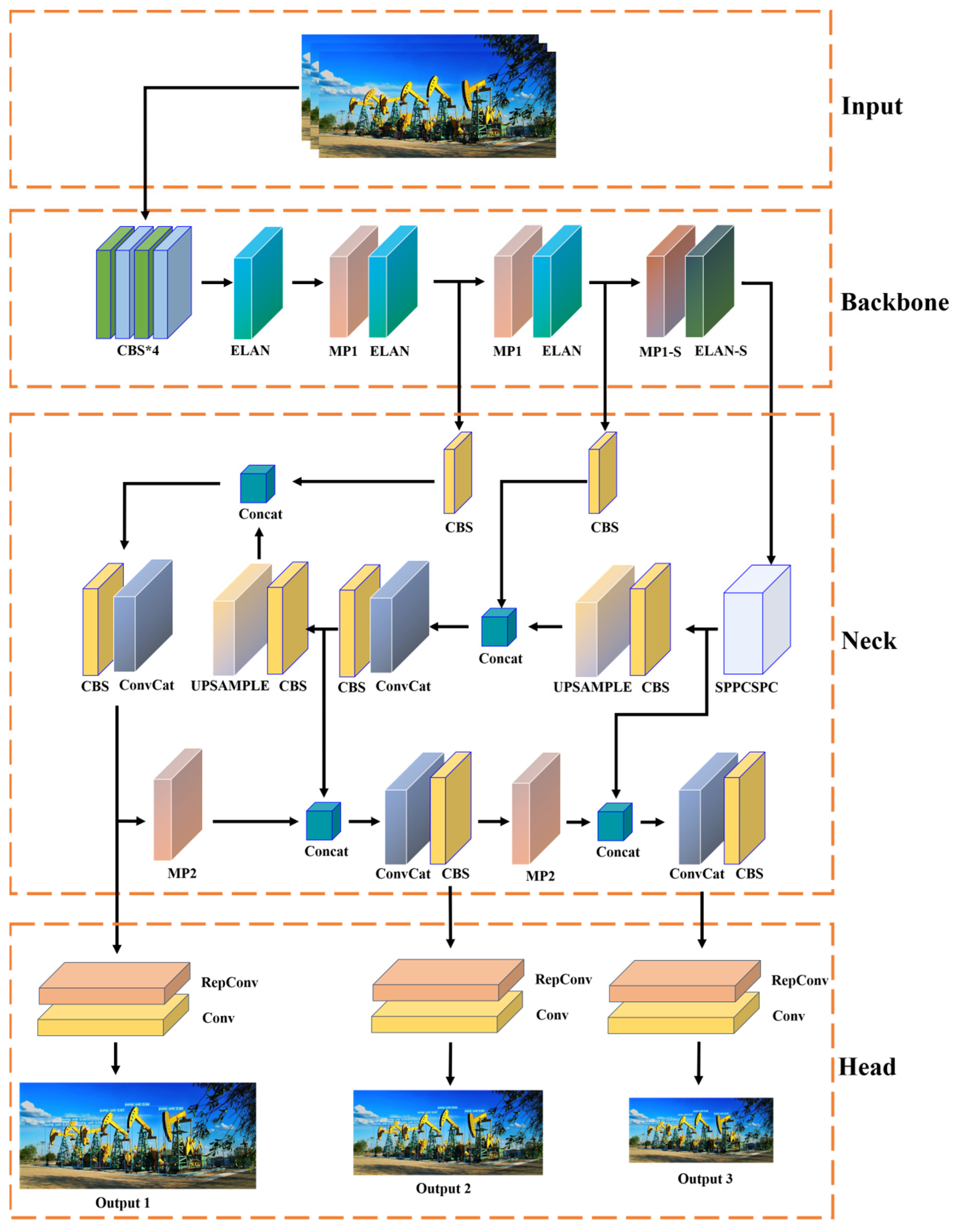
Figure 1. YOLOv7SAC network structure.
Energies 17 00835 g001
Figure 2. Structural diagram of YOLOv7SAC module.
Energies 17 00835 g002
Figure 3. Schematic diagram of switchable atrous convolution structure.
Energies 17 00835 g003
Figure 4. Schematic diagram of positive sample matching. (a) Box matching, (b) Positive sample expansion.
Energies 17 00835 g004
Figure 5. Structural diagram of head structure training strategy. (a) Auxiliary head schematic diagram, (b) Head loss fusion.
Energies 17 00835 g005
Figure 6. Schematic diagram of CIoU calculation, with red representing GT and blue representing prediction box.
Energies 17 00835 g006
Figure 7. Model building workflow.
Energies 17 00835 g007
Figure 8. Diagram of box loss: (a) YOLOv7; (b) YOLOv7SAC.
Energies 17 00835 g008
Figure 9. Diagram of various indexes of YOLOv7SAC during training.
Energies 17 00835 g009
Figure 10. Detection results of each model in the test set, where the circle indicates the detection error or missed detection. (a) Multi-scale scene; (b) occlusion scene; (c) multi-view scene; (d) image-incomplete scene.
Energies 17 00835 g010
Table 1. Comparison diagram of model indicators.
ModelmAP (%)Precision (%)Recall (%)F1 Score (%)
YOLOv5-n92.3890.4185.8088.04
YOLOv797.7694.1595.5294.83
YOLOv7SAC98.4797.6996.2796.97
Table 2. Inference speed of pumping unit detection in complex scene.
ModelNumber of ImagesAverage Time (ms)
YOLOv5-n28012.1
YOLOv728014.2
YOLOv7SAC28013.9
Disclaimer/Publisher’s Note: The statements, opinions and data contained in all publications are solely those of the individual author(s) and contributor(s) and not of MDPI and/or the editor(s). MDPI and/or the editor(s) disclaim responsibility for any injury to people or property resulting from any ideas, methods, instructions or products referred to in the content.