Proximal Policy Optimization-Based Power Grid Structure Optimization for Reliable Splitting

Abstract

When systems experience a severe fault, splitting, as the final line of defense to ensure the stability of the power system, holds immense significance. The precise selection of splitting sections has become the current focal point of research. Addressing the challenges of a large search space and unclear splitting sections, this paper introduces a grid structure optimization algorithm based on electrical coupling degree. Firstly, employing the theory of slow coherency, a generalized characteristic analysis of the system is conducted, leading to an initial division of coherency groups. Subsequently, an electrical coupling degree index, taking into account the inertia of generators, is proposed. This index can reflect the clarity of grid splitting. Furthermore, a two-layer optimization model for grid structure is constructed, utilizing the Proximal Policy Optimization (PPO) algorithm to optimize the grid structure. This process reduces the size of the splitting space and mitigates the difficulty of acquiring splitting sections. Finally, simulation validation is performed using the IEEE-118-bus system to demonstrate the effectiveness of the proposed optimization algorithm.

1. Introduction

The rapid development of the electricity industry, while bringing convenience to our lives, has also brought numerous challenges and issues for power researchers. The power grid structure is becoming increasingly complex, and issues related to the security and stability of these systems are becoming more prominent [1,2]. In long-term practice, researchers have proposed the concept of three lines of defense for power systems to protect the security of the grid and maintain the stable operation of the power system. Among them, splitting, as the last line of defense to ensure the safe and stable operation of the power system, plays an extremely important role. When a severe fault occurs in the grid, leading to the loss of synchronism of generator units, splitting at this point can prevent widespread power outages and further escalation of accidents. Currently, the selection of splitting sections takes into account the comprehensive consideration of the power angle, voltage, and frequency stability of the subnetworks after splitting, aiming to minimize the control cost post splitting. Due to the lack of comprehensive theoretical support, existing research often utilizes objectives such as minimizing unbalanced power [3,4] and minimizing the impact on power flow [5,6] as the target functions to search for splitting sections. This is carried out to enhance the stability of the partitioned grids after splitting and minimize the need for subsequent load shedding or generation curtailment. However, looking at recent power outage incidents worldwide, splitting is still not perfect. Given the increasingly large scale of power grids nowadays, finding more suitable coherent splitting sections from the perspective of the grid structure, improving the efficiency of splitting, and delving into the mechanisms of splitting control are of great significance.

Traditional splitting control is based on offline simulation analysis or operational experience. It involves pre-determining the vulnerable sections of the power grid (usually selecting the main interconnection lines in the system) and installing splitting devices to prevent major power outage incidents. At this point, it is necessary to install splitting devices into all possible sections in the entire system where stable disruptions could occur to ensure system safety comprehensively. For power grids with tight electrical connections, flexible and unpredictable operational modes and various fault patterns can lead to different instability modes in the system. The oscillation centers between generator groups do not always align with a single or specific section. This exposes the shortcomings of traditional splitting devices, which are strong in specificity but lack adaptability.

In subsequent research, active splitting control, also known as online splitting control, emerged [7,8,9,10,11]. Active splitting control is based on real-time global information of the entire power grid, enabling real-time identification of system instability modes and the search for oscillation sections. However, when the clustering patterns of the power system are not significant, obtaining reliable trigger signals from a massive amount of fault information and actively controlling widely distributed splitting devices in real time become key challenges in such studies. Slow coherency theory, as an effective tool for studying online coherence grouping in systems, has gained widespread attention both domestically and internationally [12,13,14].

In reference [12], the generalized characteristic analysis method was used to identify patterns, and the obtained weakly connected cutsets are considered to be candidate spaces for splitting decisions, reducing the search space for optimal splitting sections. Reference [15] employed the slow coherency method to identify minimal coherent generator groups. It then used graph theory, combined with the division of coherent groups, to transform the power grid into a simplified network to solve. The spectral decomposition method was then applied to select splitting sections. Reference [16], starting from the slow coherency theory, derived a strong correlation between weakly connected lines and slow mode eigenvalues in the decomposed and aggregated regions of the system. It also identifies a weak correlation between lines within coherent groups and slow mode eigenvalues. Based on this, the sensitivity of lines to slow mode eigenvalues is calculated to filter weakly connected lines. This method does not require partitioning the system node modes, making it computationally simpler, but it may have limitations in accurately selecting weakly connected lines and relies somewhat on manual judgment based on grid topology. Reference [17] began with the slow coherency theory and pointed out that differences in inter-group node correlations are a significant cause of non-convergence in splitting strategies. It explores node types to define a splitting decision space, facilitating the rapid determination of splitting sections. However, it still does not fully address the problem of widely scattered splitting in large-scale power grids. Reference [18] addressed the issue of unclear node classification during splitting by conducting modal analysis on the system to determine inter-node correlations. It proposes node classification criteria for accurate differentiation, resulting in an appropriate splitting space. Reference [19] extended artificial intelligence to traditional transmission network planning and introduced a transmission network expansion planning method based on reinforcement learning theory. Reference [20], based on slow coherency theory, presented an improved method for identifying and filtering weakly connected lines. It defines a weak connection coefficient as the ratio of weakly connected lines to the total number of lines and establishes a two-layer planning model for transmission networks considering splitting control, with the minimum weak connection coefficient as the optimization goal. Reference [21] addressed the challenge of non-convergence in splitting strategies due to the insignificance of clustering patterns during the splitting process. It proposed a grid structure optimization method based on node correlation to reduce the difficulty of splitting by adjusting the number of line branches. However, it still needs to consider differences in generator inertia and improve node classification.

This paper begins by introducing the principles and steps of the generalized characteristic analysis method. It uses this method to obtain a correlation matrix that characterizes the basis for system clustering. Then, based on the correlation matrix and the inertia parameters of each generator, an electrical coupling degree index is constructed to reflect the clarity of splitting. Subsequently, a two-layer grid structure optimization model is established, with the lower layer being a splitting section-solving model and the upper layer being a grid structure optimization model. Using the Proximal Policy Optimization (PPO) algorithm, the grid structure is optimized to reduce the splitting space and improve the efficiency of selecting splitting sections. Finally, the IEEE-118-bus system is subjected to fault simulation using the PSASP power system simulation software (Version 7.50.03). The proposed grid structure optimization algorithm is applied to optimize the grid structure, and a comparison is made between the size of the splitting space and the clarity of the selected splitting sections before and after optimization. This validates the feasibility and effectiveness of the approach presented in this paper.

2. Initial Division of Coherency Groups

In practical electrical grid systems, when interconnected large power grids are subjected to certain disturbances, it can lead to the phenomenon where the generators in the system no longer rotate at the same speed in synchronization. Instead, they exhibit phenomena such as synchronous speed zones and group instability. Synchronous speed zones refer to the grouping of generator units that maintain synchronized rotor rotation in the same group after a disturbance. Group instability occurs when different synchronous groups experience desynchronization. When determining splitting sections, it is essential to consider not only generator nodes but also the coupling degree of load nodes with different generators. Therefore, in this section, based on the slow coherency theory, a generalized characteristic analysis of the system is performed to obtain a correlation matrix, which serves as the basis for the electrical coupling degree index.

2.1. Fundamental Principles of the Correlation Matrix

The differential–algebraic equation of the power system can be written as follows:

$$\left\{\begin{array}{l}\dot{x}=f(x,y)\\ \mathbf{0}=g(x,y)\end{array}\right.,$$

(1)

where $x\in R^M$ is the power system state variable and $y\in R^N$ is the algebraic variable of the power system. Linearize Equation (1) at the equilibrium point as follows:

$$\left\{\begin{array}{l}\Delta \dot{x}=A\Delta x+B\Delta y\hfill \\ \mathbf{0}=C\Delta x+D\Delta y\hfill \end{array}\right.,$$

(2)

where $A=\frac{\partial f}{\partial x}$, $B=\frac{\partial f}{\partial y}$, $C=\frac{\partial g}{\partial x}$, $D=\frac{\partial g}{\partial y}$. Equation (2) can be rewritten as follows:

$$E\left[\begin{array}{l}\Delta \dot{x}\hfill \\ \Delta \dot{y}\hfill \end{array}\right]=S\left[\begin{array}{l}\Delta x\hfill \\ \Delta y\hfill \end{array}\right],$$

(3)

where

$$\left\{\begin{array}{l}E=\left[\begin{array}{cc}{I}_M& \mathbf{0}\\ \mathbf{0}& \mathbf{0}\end{array}\right]\hfill \\ S=\left[\begin{array}{ll}A\hfill & B\hfill \\ C\hfill & D\hfill \end{array}\right]\hfill \end{array}\right.,$$

(4)

where $I_M$ is an M-dimensional unit matrix. Based on Equation (4), the steps for the node correlation matrix can be summarized as follows:

• Find the generalized eigenvalues of the generalized eigenvalue problem (S, E);
• Arrange all eigenvalues according to the absolute value of the imaginary part from smallest to largest and determine the number of dominant oscillation modes based on the maximum difference method;
• The first r eigenvalues are selected as the dominant oscillation modes, and the corresponding r-column eigenvectors form the modal matrix Vr;
• Based on the Gaussian elimination method, obtain the correlation matrix S.

The details of the correlation matrix can be found in reference [13]. It is possible to perform initial coherency grouping for each node based on the correlation matrix S.

2.2. Classification of Nodes

The node correlation matrix $S_{ij}$ represents the correlation of node i to the coherency group j. If row i of the correlation matrix S satisfies the following condition:

$$\left\{\begin{array}{l}‖S_{i*}‖>\epsilon \\ \frac{\left|S_{ik}\right|}{‖S_{i*}‖}>\xi \end{array}\right.,$$

(5)

Then, node i is a mode node belonging to coherency group k; otherwise, node i is a fuzzy node. In the formula, ε and ξ are positive numbers less than 1, which can be flexibly adjusted to determine the node mode according to the actual scenario.

When determining splitting sections in the network topology, nodes belonging to the same mode group of nodes must be grouped in the same region. Fuzzy nodes, on the other hand, can be grouped in any group since they have low correlations with all mode groups.

3. Two-Layer Grid Structure Optimization Model Based on Electrical Coupling Degree Index

In order to enhance the ability of the power grid to withstand severe faults and prevent the occurrence of large-scale cascading failures, it is necessary to predefine splitting sections to divide the power grid into sub-regions in the early stages of a fault to prevent the spread of the fault. However, if the units within each region cannot operate in synchronization after splitting, it can still lead to oscillations within the regions, thereby reducing the overall system stability. Therefore, it is necessary to establish an upper-level grid structure optimization model that takes into account the electrical coupling degree index and a lower-level splitting section search model that considers the electrical coupling degree and minimum imbalance power.

3.1. Lower-Level Splitting Section Solving Model

Let the nth order undirected graph of the jth coherency group after splitting be represented as G_j = (V_j,E_j), V_j is all the nodes belonging to the jth coherency group, and E_j is the edges formed by all the nodes belonging to each of the jth coherency groups.

3.1.1. Objective Function

The objective function of the lower-level optimization model is

$$f_l=\min \left({\displaystyle \sum _{j=1}^k{P}_{j,un}}-I_{CH}\right),$$

(6)

where $P_{j,un}$ is the unbalanced power within each of the jth coherency groups and $I_{CH}$ is the network-wide electrical coupling index. The unbalanced power of each coherency group is as follows:

$$P_{j,un}=\max \left\{{\displaystyle \sum _{i\in G_j}\left(p_i-g_i\right),0}\right\},$$

(7)

where $p_i$ represents the load magnitude of the ith node belonging to the coherency group $G_j$, and $g_i$ represents the generation output of all ith nodes belonging to the coherency group $G_j$. Max{a,b} denotes selecting the larger value between a and b. This equation calculates the value of loads within the coherency group that exceeds the total generation capacity. This portion of the load is cut off due to insufficient generation and is minimized as an objective function during optimization.

The specific expression of $I_{CH}$ is as follows:

$$I_{CH}=\frac{{\displaystyle {\sum }_{k=1}^t\left({\sum }_{i\in C_k}{J}_i\right){‖u_k-u‖}^2/(t-1)}}{{\displaystyle {\sum }_{k=1}^t{\displaystyle {\sum }_{x\in C_k}{‖x_i-u_k‖}^2{J}_i}}},$$

(8)

$$u=\frac{{\displaystyle {\sum }_{i=1}^n{J}_i}{u}_i}{{\displaystyle {\sum }_{i=1}^n{J}_i}},u_k=\frac{{\displaystyle {\sum }_{i\in C_k}{J}_i}{u}_i}{{\displaystyle {\sum }_{i\in C_k}{J}_i}},$$

where u is the mean value of correlation of all generator nodes after considering inertia; $u_k$ is the mean value of correlation of generator nodes in the kth region after considering inertia; $C_k$ is the set of generator nodes in the kth region; t is the number of regions; $J_i$ is the inertia of the ith generator, $x_i$ is the correlation of the ith generator; and $u_i$ is the correlation of the ith generator node.

This index essentially represents the ratio of the distance between different coherency groups to the distance within each coherency group. It can reflect the closeness within regions and the distinguishability between different regions.

3.1.2. Constraint Conditions

• Upper and lower voltage constraints.

After partitioning the regions, the voltage of nodes within each region should be maintained within the upper and lower limits:

$$V_{\min }\le V_i\le V_{\max },$$

(9)

where $V_i$ is the voltage at node i, and the $V_{\min }$ and $V_{\max }$ distributions indicate the upper and lower limits of the node voltage.

• Line transmission power limitations.

The transmission power of each line must not exceed its line capacity limit after unlinked operation:

$$P_i^L\le P_{i,\max }^L,$$

(10)

where $P_i^L$ is the transmission power on line i and $P_{i,\max }^L$ is the upper limit of transmission power on line i.

• Connectivity constraints.

This paper is based on Warshall’s algorithm to determine the connectivity of a graph. Let $A_j$ be the adjacency matrix of the graph $G_j$, then the reachability matrix of the graph is as follows:

$$R_j={\displaystyle \sum _{i=1}^{n_j}{A}_j^i},$$

(11)

If all the elements of the reachability matrix $R_j$ are greater than 0, the undirected graph nodes are said to be reachable to each other and satisfy the connectivity constraints of the graph, otherwise the connectivity constraints are not satisfied.

3.2. Upper-Level Grid Structure Optimization Model

In the upper-level grid structure optimization model, the new grid structure is sent to the lower model for slow coherency group division by disconnecting or filling the original line, and the value of the objective function is obtained after splitting. Objective function:

$$f_u=\min \left(f_l-k_v{V}_s\right),$$

(12)

where $f_u$ is the objective function of the upper optimization model, $V_s$ is the voltage stability index of the whole network, and $k_v$ is the weight parameter. Combined with the actual grid operation, a certain voltage stability needs to be considered at the same time. The specific expression of $V_s$ is as follows:

$$V_s=\min \left\{{\lambda }_1,{\lambda }_2,\dots ,{\lambda }_n\right\},$$

(13)

where λ₁λ₂,..., λ_n are the eigenvalues of the reduced-order Jacobi matrix, and the smallest eigenvalue is selected as the magnitude of voltage stability. The objective function of the upper-level grid structure optimization model is a multi-objective optimization problem that takes into account both the electrical coupling degree index and voltage stability.

The upper-level grid structure optimization model constraints are similar to the constraints in the lower-level splitting section solving model, as shown in Equations (9)–(11).

4. Optimization of Grid Structure Based on Proximal Policy Optimization Algorithm

4.1. Principles of the Proximal Optimization Algorithm

Reinforcement learning has a stronger global search ability when dealing with sequence optimization problems compared with traditional intelligent algorithms, which is conducive to finding the global optimal solution. Power system grid structure optimization is a sequential optimization problem, which is suitable to solve through the use of reinforcement learning algorithms. Among the various reinforcement learning algorithms, the Proximal Optimization Algorithm (PPO) can solve discrete high-dimensional action problems, and the online strategy can learn excellent solutions quickly and efficiently and has shown excellent performance in the public dataset, so the PPO algorithm is chosen to solve the power system grid structure optimization problem.

4.1.1. Setting of the Reward Function

The reward function setting of reinforcement learning is very important, which directly determines the goodness of the policy network obtained from the final training. Different reward functions need to be set reasonably for different problems.

This task requires comprehensive consideration of the electrical coupling index and voltage support index of the power grid. Therefore, the reward is set as the increment of the comprehensive evaluation of the two indicators after each addition of lines, and the formula is shown below:

$$r_t=(I_{CH,t}+V_{s,t})-(I_{CH,t-1}+V_{s,t-1}),$$

(14)

where $r_t$ denotes the reward at step t, $I_{CH,t}$ and $I_{CH,t-1}$ denote the electrical coupling indexes at step t and step t − 1, respectively, and $V_{s,t}$ and $V_{s,t-1}$ denote the voltage support indexes at step t and step t − 1, respectively.

$$V_s=\min \left\{{\lambda }_1,{\lambda }_2, \dots ,{\lambda }_n\right\},$$

(15)

where λ₁λ₂,..., λ_n are the eigenvalues of the reduced order Jacobi matrix, and the smallest of these eigenvalues is selected as the voltage stability index.

4.1.2. TD-Error

Temporal-difference error (TD-error) is an error function calculation method used to update the value function. The principle is that the estimation of the value function is made more accurate by replacing the estimated value with a partially true value ($r_t$).

$$V(s_t)\leftarrow V(s_t)+\alpha [r_{t+1}+\gamma V(s_{t+1})-V(s_t)],$$

(16)

where $V\left(s_{t+1}\right)$ and $V\left(s_t\right)$ denote the state value function estimates at step t + 1 and step t, respectively; γ is the decay coefficient, and α is the learning rate.

The meaning of this equation is to use the known reward value and the value function estimate of the next step to replace the current value function estimate in order to make the current value function estimate more accurate.

4.1.3. Generalized Advantage Estimation

The dominance function is the dominance of an action a in state s over the average. Let:

$${\delta }_t=r_t+\gamma V(s_{t+1})-V(s_t),$$

(17)

If $V\left(s_t\right)$ could be completely accurate and unbiased, then the equation could be used directly as an advantage function, indicating the advantage of the current action over the average action. However, $V\left(s_t\right)$ is obtained indirectly from the neural network and cannot be unbiased, then one can only keep refining $V\left(s_{t+1}\right)$ to make it as unbiased as possible.

Therefore, Generalized Advantage Estimation (GAE) expands $V\left(s_{t+1}\right)$ to form the following equation:

$$\begin{array}{l}{A}_t=r_t+\gamma (r_{t+1}+\gamma V(s_{t+2}))-V(s_t)\\ \hspace{1em}\hspace{0.17em}=r_t+\gamma (r_{t+1}+\gamma (r_{t+2}+V(s_{t+3})))-V(s_t)\\ \hspace{1em}\hspace{0.17em}=\dots \\ \hspace{1em}\hspace{0.17em}=-V(s_t)+{\displaystyle \sum _{l=0}^{\infty }{\gamma }^l{r}_{t+l}}\hspace{1em}\hspace{1em}\hspace{1em}\hspace{1em}\hspace{1em}\hspace{1em}\hspace{1em}\hspace{1em},\end{array}$$

(18)

where $A_t$ is the dominance function of GAE(γ, 1), who is the unbiased estimation of the action $A_t$. Compared with other reinforcement learning algorithms, PPO adopts the generalized dominance estimation as the dominance function, and by reasonably choosing the value of γ, the variance can be greatly reduced with acceptable bias, which enables the value function to converge effectively.

4.1.4. PPO-Clip

The traditional strategy gradient algorithm uses the following equation as the loss of the strategy network:

$$\widehat{g}={\widehat{\mathbb{E}}}_{\mathrm{t}}\left[{\nabla }_{\theta }\log {\pi }_{\theta }\left(a_t|s_t\right){\widehat{A_t}}^{\mathrm{t}}\right],$$

(19)

where $\widehat{g}$ denotes the loss function value and ${\pi }_{\theta }$ denotes the network strategy. Then, the Monte Carlo approximation of $\log {\pi }_{\theta }(a_t\left|s_t){\widehat{A}}_t^t\right.$ is computed and backpropagated to update the strategy network. However, it is easy for the number to be too large, resulting in the difference between the old and new network strategies being too large and difficult to converge. PPO-clip compares the difference between the old and new networks, and if the difference is too large, the update is not performed. The policy network loss values for PPO-clip are defined as follows:

$$r_t(\theta )=\frac{{\pi }_{\theta }\left(a_t|s_t\right)}{{\pi }_{{\theta }_{\mathrm{old} }}\left(a_t|s_t\right)},$$

(20)

$${\mathrm{L}}^{\mathrm{CLIP}}(\theta )={\widehat{\mathbb{E}}}_{\mathrm{t}}\left[\min \left(r_t(\theta ){\widehat{\mathrm{A}}}_{\mathrm{t}},\mathrm{clip}\left(r_t(\theta ),1-ϵ,1+ϵ\right){\widehat{\mathrm{A}}}_{\mathrm{t}}\right)\right],$$

(21)

where ${\pi }_{\theta }$ denotes the new network strategy, ${\pi }_{{\theta }_{old}}$ denotes the old network strategy, and clip is a limiting function that limits $r_t(\theta )$ to between 1 − ϵ and 1 + ϵ. The relationship between $r_t(\theta )$ and ${\mathrm{L}}^{\mathrm{CLIP}}(\theta )$ is analyzed as shown in Figure 1.

It can be seen that when A > 0, this backpropagation will not have an effect on the weights as long as the ratio of the current strategy ${\pi }_{\theta }$ under action $a_t$ compared to the pre-update ${\pi }_{{\theta }_{old}}$ is too large, i.e., more than 1 + ϵ, and according to the functional relationship in the figure, it can be seen that the gradient of the loss about r is 0. On the contrary, when A < 0, if the update ratio is less than 1 − ϵ, it means that the update is too large and will not have an effect on the weights.

In other words, the update is performed only when the new network is not too different from the old one; otherwise, the network is not updated. Compared with other reinforcement learning algorithms, PPO adopts the PPO-clip strategy to effectively avoid the non-convergence problem that may be caused by an update of the network parameters that is too large.

4.2. Solution Process of the Grid Structure Two-Layer Model

The grid topology optimization based on the PPO algorithm is illustrated in Figure 2.

• The policy network interacts with the environment. First, the environment provides the current state to the policy network, which includes the current grid information and the electrical coupling index within the current grid. The policy network then outputs an action, which involves either adding or removing lines from the existing grid. Additionally, the policy network also outputs a value function for the current state. After receiving the action, the environment updates the state, which involves modifying the grid structure. During this process, the environment records intermediate variables such as the state before and after the action, the action itself, the value function, and other relevant information;
• After meeting the end conditions, based on the recorded process quantities, train the policy function in the policy network based on generalized dominance estimation and PPO-clip, and train its value function based on TD-error and mean square error;
• Terminate after satisfying the preset number of loops and output the final grid structure optimization scheme.

5. Case Study

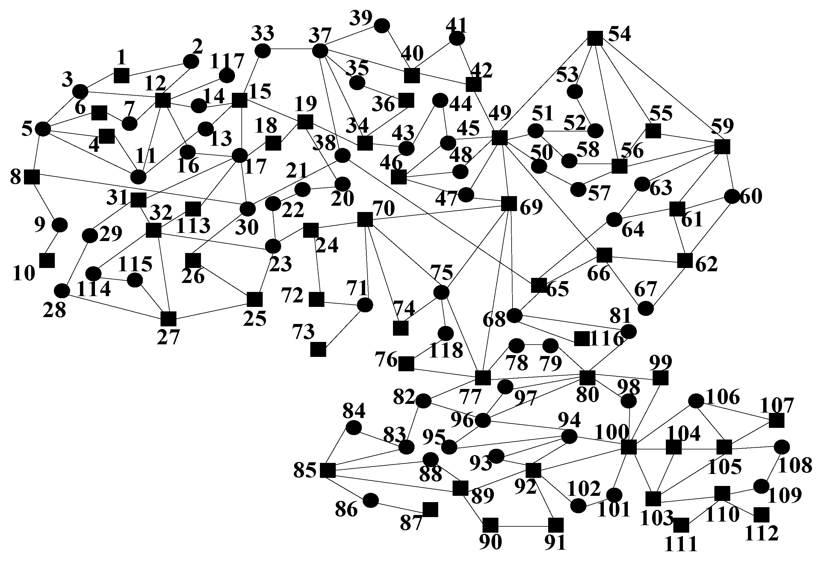
To validate the proposed grid structure optimization solution, it is tested on the IEEE-118-bus system. The IEEE-118-bus system comprises 186 transmission lines and 54 generators. The system topology is depicted in Figure 3.

In the diagram, the black square boxes represent generator nodes, which are modeled using a fifth-order model. The black circular nodes represent load nodes, which are modeled as constant power loads. In MATLAB (Version 2021b), a system’s generalized eigenvalue matrix was constructed, and the number of regions for system partitioning was determined to be three, as per the content of Section 2. The reference variables for the three regions are the phase angles at nodes 1, 80, and 111. Region 1 is defined as the region where node 1 belongs, and all generator units within this group form Region 1’s units. Region 2 is defined as the region where node 80 belongs, and all generator units within this group form Region 2’s units. Region 3 is defined as the region where node 111 belongs, and all generator units within this group form Region 3’s units.

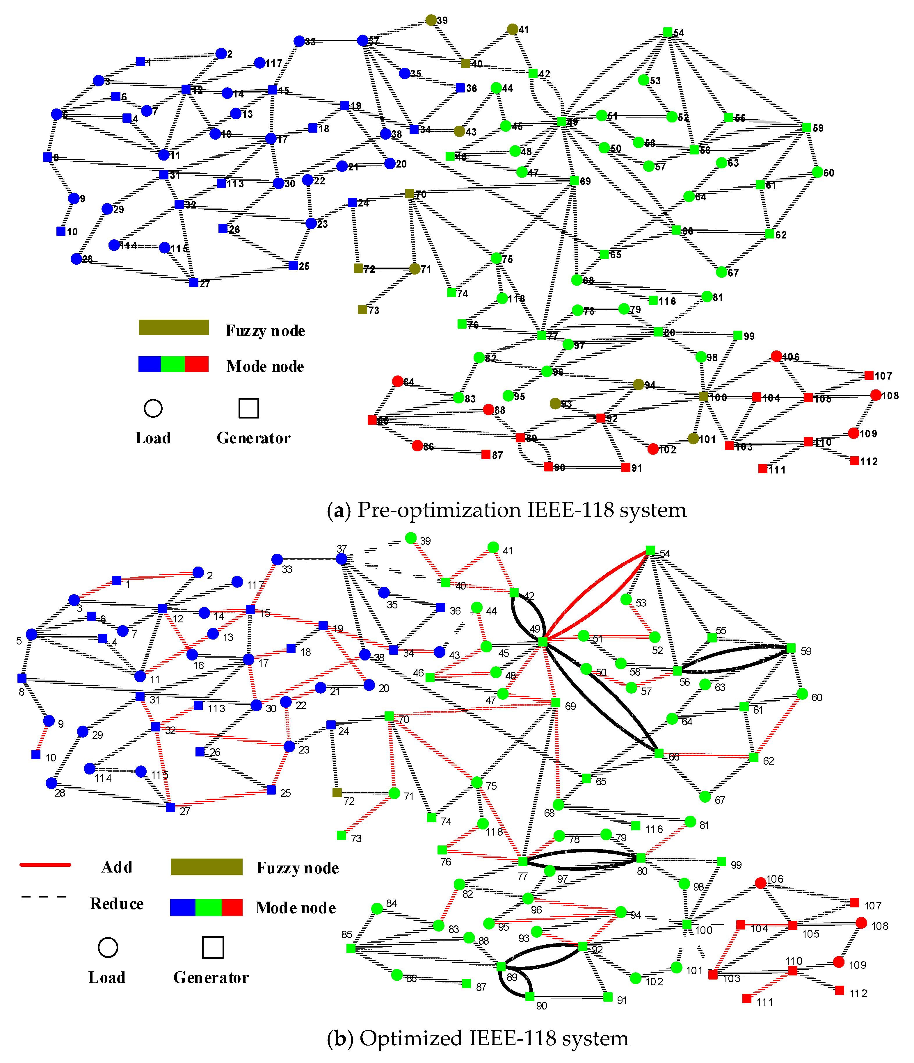
Using the grid structure two-layer optimization program proposed in Chapters Three and Four, the optimized grid and node classification for the IEEE-118 system were obtained. A comparison between the grid structure before and after optimization is shown in Figure 4.

After optimization, 61 new transmission lines were added, as indicated by the red lines in the diagram, and 8 lines were disconnected, as represented by the dashed lines in the diagram. Before optimization, the upper-level index was 44, and the electrical coupling index was 65. After optimization, the upper-level index improved to 185, and the electrical coupling index increased to 233, indicating a significant enhancement in electrical coupling. From the perspective of node types, after optimization, the mode nodes become more concentrated. In particular, the nodes of mode 3, which were originally scattered, have now shifted to a more centralized distribution. This concentration is beneficial for the angular stability and qualitative analysis of the grid’s islands after splitting. The number of fuzzy nodes has decreased from 12 to 1, significantly reducing the fuzzy space. As a result, the overall solution space for splitting has effectively reduced, which facilitates the determination of splitting sections. This demonstrates that the two-layer grid structure optimization model proposed in this paper can effectively reduce the splitting space and lower the splitting difficulty.

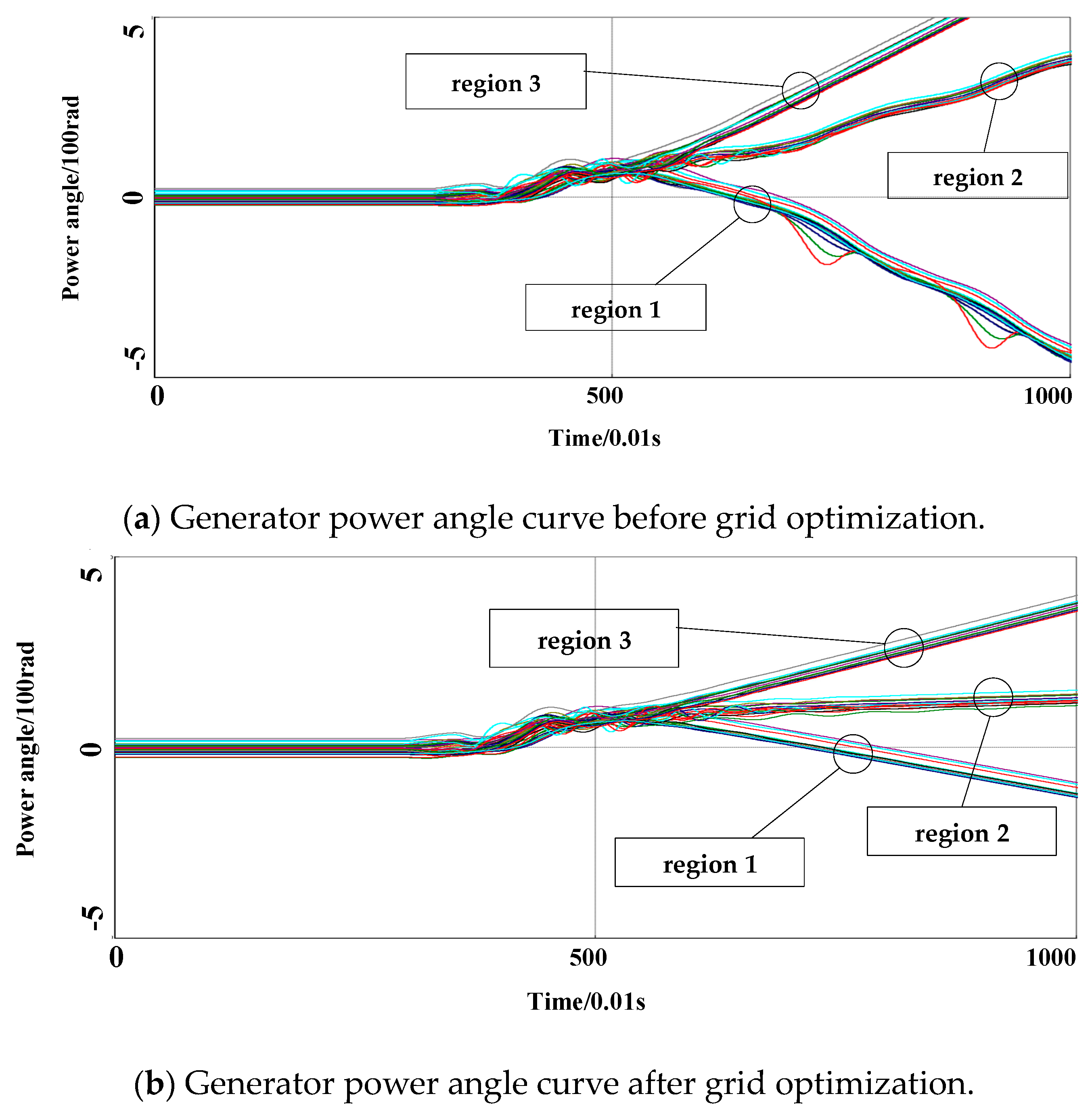
Next, we subjected both the pre-optimized and post-optimized grids to the same fault that caused the system to become unstable. The fault was set as follows: a three-phase ground short circuit fault occurred in lines 80–81 at 3 s and was cleared at 3.5 s. Using the minimum unbalanced power as the objective function, we performed splitting on the pre-optimized and post-optimized grids at 5 s. The power angle curves for each generator are shown in Figure 5.

Comparing the generator power angle curves before and after grid optimization, it can be observed that after applying the same fault to the power grid, both the original grid and the optimized grid, based on the slow coherency theory, still maintain synchronous operation within their respective mode groups, and no desynchronization occurs. This indicates that grid optimization can ensure the stability of the system after splitting while reducing the splitting space and difficulty. Furthermore, comparing the power angle curves for Region 1 generators before and after optimization, it can be seen that although this group could maintain synchronization after splitting in the pre-optimized grid, there were some generators experiencing various degrees of oscillations. However, after optimization, this group’s synchronization characteristic is much more stable. This demonstrates the effectiveness of the grid optimization program proposed in this paper.

6. Conclusions

This paper, by considering the distribution of nodes and the impact of generator inertia on the selection of splitting sections, proposed a two-layer grid structure optimization method based on the electrical coupling index using the PPO algorithm. It has successfully achieved the effect of reducing the splitting space, making the selection of splitting sections clearer, and lowering the difficulty of splitting. The main conclusions are as follows:

• The correlation matrix obtained through generalized characteristic analysis can reflect the clarity of splitting. When considering generator inertia, the proposed electrical coupling index provides a clear and intuitive representation of the splitting difficulty in different systems.
• By changing the grid structure, such as adding or removing certain lines in the system, the size, clarity, and difficulty of splitting space can be altered. The two-layer optimization model based on the PPO algorithm can effectively optimize the system’s grid structure to reduce the splitting space and lower the difficulty of splitting.
• Compared to existing methods that rely solely on slow coherency theory to determine the splitting spaces, the grid structure optimization method proposed in this paper, based on the PPO algorithm, goes beyond slow coherency theory. It not only ensures reliable splitting of the grid but also further reduces the size of the splitting space. This method provides power grid planners with an effective approach to grid planning.

References

- Yun, L. Analysis on Out-of-step Separation in Brazilian Power Grid and Its Inspiration. Power Syst. Technol. 2019, 43, 1111–1121. [Google Scholar]
- Weifang, L.; Yong, T.; Huadong, S.; Qiang, G.; Hongguang, Z.; Bing, Z. Blackout in Brazil Power Grid on February 4, 2011 and Inspirations for Stable Operation of Power Grid. Autom. Electr. Power Syst. 2011, 35, 1–5. [Google Scholar]
- Najafi, S. Evaluation of interconnected power systems controlled islanding. In Proceedings of the 2009 IEEE Bucharest PowerTech, Bucharest, Romania, 28 June–2 July 2009; pp. 1–8. [Google Scholar]
- Wang, C.G.; Zhang, B.H.; Hao, Z.G.; Shu, J.; Li, P.; Bo, Z.Q. A Novel Real-Time Searching Method for Power System Splitting Boundary. IEEE Trans. Power Syst. 2010, 25, 1902–1909. [Google Scholar] [CrossRef]
- Yang, B.; Vittal, V.; Heydt, G.T.; Sen, A. A Novel Slow Coherency Based Graph Theoretic Islanding Strategy. In Proceedings of the 2007 IEEE Power Engineering Society General Meeting, Tampa, FL, USA, 24–28 June 2007; pp. 1–7. [Google Scholar]
- Ding, L.; Gonzalez-Longatt, F.M.; Wall, P.; Terzija, V. Two-Step Spectral Clustering Controlled Islanding Algorithm. IEEE Trans. Power Syst. 2013, 28, 75–84. [Google Scholar] [CrossRef]
- Chen, S.; Jiayun, W.; Ying, Q.; Qiang, L.; Qianjin, L.; Rehtanz, C. Studies on Active Splitting Control of Power Systems. Proc. Chin. Soc. Electr. Eng. 2006, 26, 1–6. [Google Scholar]
- Yongjie, F. Adaptive Islanding Control of Power Systems. Autom. Electr. Power Syst. 2007, 31, 41–44,48. [Google Scholar]
- Senroy, N.; Heydt, G.T. A conceptual framework for the controlled islanding of interconnected power systems. IEEE Trans. Power Syst. 2006, 21, 1005–1006. [Google Scholar] [CrossRef]
- You, H.; Vittal, V.; Wang, X. Slow coherency-based islanding. IEEE Trans. Power Syst. 2004, 19, 483–491. [Google Scholar] [CrossRef]
- Sun, K.; Zheng, D.; Lu, Q. A simulation study of OBDD-based proper splitting strategies for power systems under consideration of transient stability. IEEE Trans. Power Syst. 2005, 20, 389–399. [Google Scholar] [CrossRef]
- Jingmin, N.; Chen, S.; Qian, C. Adaptive controlled islanding based on slow coherency—Part I: Research on the theoretical basis. Proc. Chin. Soc. Electr. Eng. 2014, 34, 4374–4384. (In Chinese) [Google Scholar]
- Jingmin, N.; Chen, S.; Qian, C. Adaptive islanding control based on slow coherency—Part II: Practical area partition method. Proc. Chin. Soc. Electr. Eng. 2014, 34, 4865–4875. (In Chinese) [Google Scholar]
- Jingmin, N.; Chen, S.; Qian, C. Adaptive islanding control based on slow coherency—Part III: Design of the practical scheme. Proc. Chin. Soc. Electr. Eng. 2014, 34, 5597–5609. (In Chinese) [Google Scholar]
- Song, H.; Wu, J.; Wu, L. Controlled islanding based on slow-coherency and KWP theory. In Proceedings of the 2012 IEEE Innovative Smart Grid Technologies-Asia(ISGT Asia), Tianjin, China, 21–24 May 2012; IEEE: Piscataway, NJ, USA, 2012; pp. 1–6. [Google Scholar]
- Jingmin, N.; Chen, S.; Ying, L.; Wei, T. An On-line Weak-connection Identification Method for Controlled Islanding of Power System. Proc. Chin. Soc. Electr. Eng. 2011, 31, 24–30. [Google Scholar]
- Ying, Q.; Chen, S.; Qiang, L. Islanding Decision Space Minimization and Quick Search in Case of Large-scale Grids. Proc. Chin. Soc. Electr. Eng. 2008, 28, 23–28. [Google Scholar]
- Shuangteng, H.; Xinwei, S.; Yuhong, W.; Zongsheng, Z.; Xi, W.; Peng, S.; Yunxiang, S.; Yao, H. A method for searching splitting surface considering network splitting adaptation index. IET Signal Process. 2023, 17, e12197. [Google Scholar]
- Yuhong, W.; Shengjie, H.; Yuyan, S.; Li, J.; Li, S. Transmission Expansion Planning Based on Reinforcement Learning. Power Syst. Technol. 2021, 45, 2829–2838. [Google Scholar]
- Chufei, Y.; Fei, T.; Dichen, L.; Hongsheng, Z.; Xiongguang, Z.; Weiqiang, L.; Wen, J. Transmission Network Expansion Planning Considering Disjoint Control. Power Syst. Technol. 2020, 44, 2204–2215. [Google Scholar]
- Weiqiang, F.; Fei, T.; Fusuo, L.; Dichen, L.; Chufei, X.; Jiale, L.; Gucheng, X. Research on the Structure Optimization of Grid Frame Based on Node Correlation Analysis for Reliable Splitting. Proc. Chin. Soc. Electr. Eng. 2020, 40, 731–743. [Google Scholar]