Abstract
This study investigates the non-destructive analysis of proximate parameters (moisture content, MC; volatile matter, VM; fixed carbon, FC; ash content) in various chipped and ground biomass using a combination of destructive thermogravimetric analysis (TGA) and non-destructive near-infrared spectroscopy (NIRS) with partial least squares regression (PLSR). The thermogravimetric method determines proximate analysis data through TG and DTG curves, tracking biomass mass loss over time or temperature. NIRS scans chipped biomass in diffuse reflectance, and ground biomass in transflectance mode, covering the wavenumber range from 3595 to 12,489 cm−1. PLSR-based models (Full-PLSR, GA-PLSR, SPA-PLSR, MP PLSR 5-range method, and MP PLSR 3-range method) are developed and evaluated based on R2P, RMSEP, and RPD. MC and FC models for chip biomass exhibit satisfactory performance, making them cautiously applicable in various applications, including research. Optimal models for MC and FC in chip biomass, constructed using GA-PLSR with the second derivative and Full-PLSR with a constant offset, yield high R2P values (0.8654 and 0.8773), low RMSEP values (0.85% and 2.12%), and high RPD values (2.9 and 3.0), indicating applicative capabilities. Other parameters such as MC and FC in ground biomass, as well as VM and ash content in both chip and ground biomass, are found suitable for rough screening. Model sensitivity, assessed by calculating LOQ, indicates high sensitivity for VM in both chip and ground biomass and FC in chip biomass, as the calculated LOQ value is lower than the minimum reference values used during model development. However, for the remaining parameters, LOQ values surpass the established minimum reference value, suggesting limitations in predicting samples below the calibration range. Continuous model enhancement incorporating an ample number of representative biomass samples and consistent validation with unknown samples are imperative for ensuring accurate predictions.
1. Introduction
Biomass is a renewable, carbon neutral, abundantly available, and sustainable energy source that holds the potential to reduce or replace reliance on fossil fuels, contributing to energy savings and environmental preservation [1]. Studies indicate that the global production of lignocellulosic biomass, including crop residues, wood, and grass, amounts to approximately 181.5 billion tonnes each year [2]. This highlights the substantial potential of utilizing agricultural residues and wood from fast-growing trees for bio-conversion. A primary concern is that biomass generally has a lower energy density compared to fossil fuels. Nevertheless, the application of diverse biomass energy technologies rooted in thermochemical treatments, namely, pyrolysis (300 to 1000 °C), gasification (500 to 1300 °C), liquefaction (250 to 550 °C), torrefaction (200 to 300 °C), and combustion (700 to 1000 °C) displays the potential to effectively transform biomass into valuable energy resources [3,4].
The wide range of biomass sources, the diverse assortment of agricultural and tree waste materials, and the continuous variations in their properties during processing, storage, and transportation collectively pose challenges in effectively characterizing and understanding biomass as an efficient fuel. The characterization of biomass is crucial for reliably predicting its behavior as a fuel [5]. In the context of the thermal conversion of biomass, proximate analysis emerges as a pivotal method for characterization [4]. Proximate analysis is used to determine the mass percentages on a wet basis of MC, VM, FC, and ash content, all of which significantly influence both combustion behavior and plant design.
During the biomass combustion process, the rate of heat release is primarily influenced by proximate analysis parameters, including MC, VM, FC, and ash content [6]. Adjustments in these proximate analysis values can yield variations in crucial combustion performance indicators such as ignition time and temperature, burnout time and temperature, and the overall heat release. Higher moisture levels decrease the higher heating value of biomass [7] and lead to reduced combustion efficiency, whereas higher ratios from VM to FC correspond to increased fuel reactivity [8]. VM refers to the components in biomass that are converted into a gaseous form through thermal decomposition, whereas FC represents the non-volatile segment of the biomass. A high VM content does not necessarily ensure a high calorific value because some VM constituents are derived from non-combustible gases like CO2 and H2O. Lower MC and VM contents contribute to the improvement of the FC content in biomass samples [9]. A high FC signifies a higher carbon content in the biomass, resulting in higher energy content and generating maximum heat during combustion [10]. Therefore, the FC content of biomass positively influences its energy potential and calorific value. Conversely, a higher presence of VM in the biomass results in lower FC, consequently impacting the energy potential of the biomass negatively.
Ash is an inorganic residue that remains after ignition of combustible substance [11,12]. The energy required for the thermal breakdown and phase transition of ash-forming inorganics is extracted from the biomass burning energy, resulting in a reduction in calorific value [13]. The presence of high MC and elevated ash content in biomass leads to ignition and combustion problems [5]. Also, the presence of ash influences corrosion and slag formation [8].
Various standard procedures exist to measure these proximate analysis parameters. ASTM E871-82 (2019) [14] addresses moisture, ASTM E872-82 (2019) [15] handles volatile matter, and ASTM E1755-01 (2020) [16] tackles ash in biomass. FC is usually determined by calculating the difference between 100% and the sum of MC, VM, and ash content [12,17]. These standard methods are involved in heating a sample under specific conditions and assessing the change in weight. For proximate analysis of biomass, experimentation includes using a simple oven to determine MC and a furnace to determine VM and ash contents. The experimental techniques employed to estimate these parameters often consume considerable time, are financially demanding, and carry an increased likelihood of experimental error. Additionally, considering the large number of samples needed to determine the proximate analysis data for biomass characterization, the process is both tedious and destructive in nature. Hence, various researchers have recommended the use of TGA for the proximate analysis of biomass. For instance, Posom et al. (2020) recommend the use of TGA to determine the proximate analysis of bamboo chip and leucaena pellets biomass [18], Torquato et al. (2017) investigated the appropriate conditions for determining proximate parameters of lignocellulosic agricultural residue using TGA [19], and García et al. (2013) analyzed 13 different types of biomass for proximate analysis using TGA [8]. Similarly, previous research studies have demonstrated the potential of utilizing NIR spectroscopy, as an alternative method, for assessing biomass proximate analysis parameters across the wavelength range between 780 and 2500 nm. Posom et al. (2022) developed a reliable and accurate model for online measurement of MC in sugarcane [20]. Toscano et al. (2022) estimated the MC of industrial wood chip fuel using a portable NIR spectrometer [21]. Sirisomboon et al. (2020) compared the performance of proximate data models, namely, MC, VM, FC, and ash, through direct scanning of bamboo chips [22]. Shrestha et al. (2018) evaluated MC in bamboo chips using diode array near-infrared spectroscopy [23]. Posom et al. (2017) determined the HHV, VM, FC, and ash content of ground bamboo using FT-NIRS [24]. Adnan et al. (2017) assessed the feasibility of NIRS and chemometrics for rapid and non-destructive prediction of MC in intact green coffee beans [25]. The above research demonstrates the potential of TGA for determining proximate parameters and NIRS for rapidly predicting biomass proximate parameters. Therefore, this study integrates TGA and NIRS, developing NIRS as an alternative method for biomass proximate analysis using calibration models with chemometrics, specifically PLSR, for rapid analysis. This enables real-time measurements and high-throughput screening of biomass samples. This approach eliminates the need for sample preparation and the use of consumables, thereby reducing costs and minimizing negative environmental impact. Additionally, it is a safe method with less operator dependency.
Although NIRS is a rapid, reliable, and non-destructive analytical method, it requires the development of individual calibration models based on spectral data and each reference parameter. This process can be time consuming and costly. However, in the long term, it proves to be beneficial for the accurate assessment of proximate analysis parameters. To the best of our knowledge, there have been no publications reporting the development of a global NIRS model for proximate parameters using fast-growing trees and agricultural residue which can be categorized into wood and non-wood biomass. Many studies on biomass and NIRS modeling have found that PLSR is a very effective and widely used method for quantitative analysis [26,27,28,29]. Therefore, in this work, we elucidate the rationale for combining both types of biomass materials for model development. Additionally, this study marks the first application of the recent MP methods, specifically the 5-range and 3-range methods, for the NIRS evaluation of proximate parameters in biomass. Therefore, the main aims of this study are as follows:
- To determine the proximate analysis parameters, i.e., MC, VM, FC, and ash content of biomass, using TGA.
- To develop separate calibration models using Full-PLSR, GA-PLSR, SPA-PLSR, the multi-reprocessing 5-range PLSR, and the multi-preprocessing 3-range PLSR for the non-destructive assessment of each proximate analysis parameter in both chipped and ground biomass.
- To compare and select the best performing PLSR-based model for each proximate analysis parameter from chipped and ground biomass, and establish it as a rapid, reliable, non-destructive alternative method for assessment of proximate analysis parameters.
- To determine the LOQ value for each proximate parameter using the calibration set of the proposed high-performance model, both for chip and ground biomass.
2. Materials and Methods
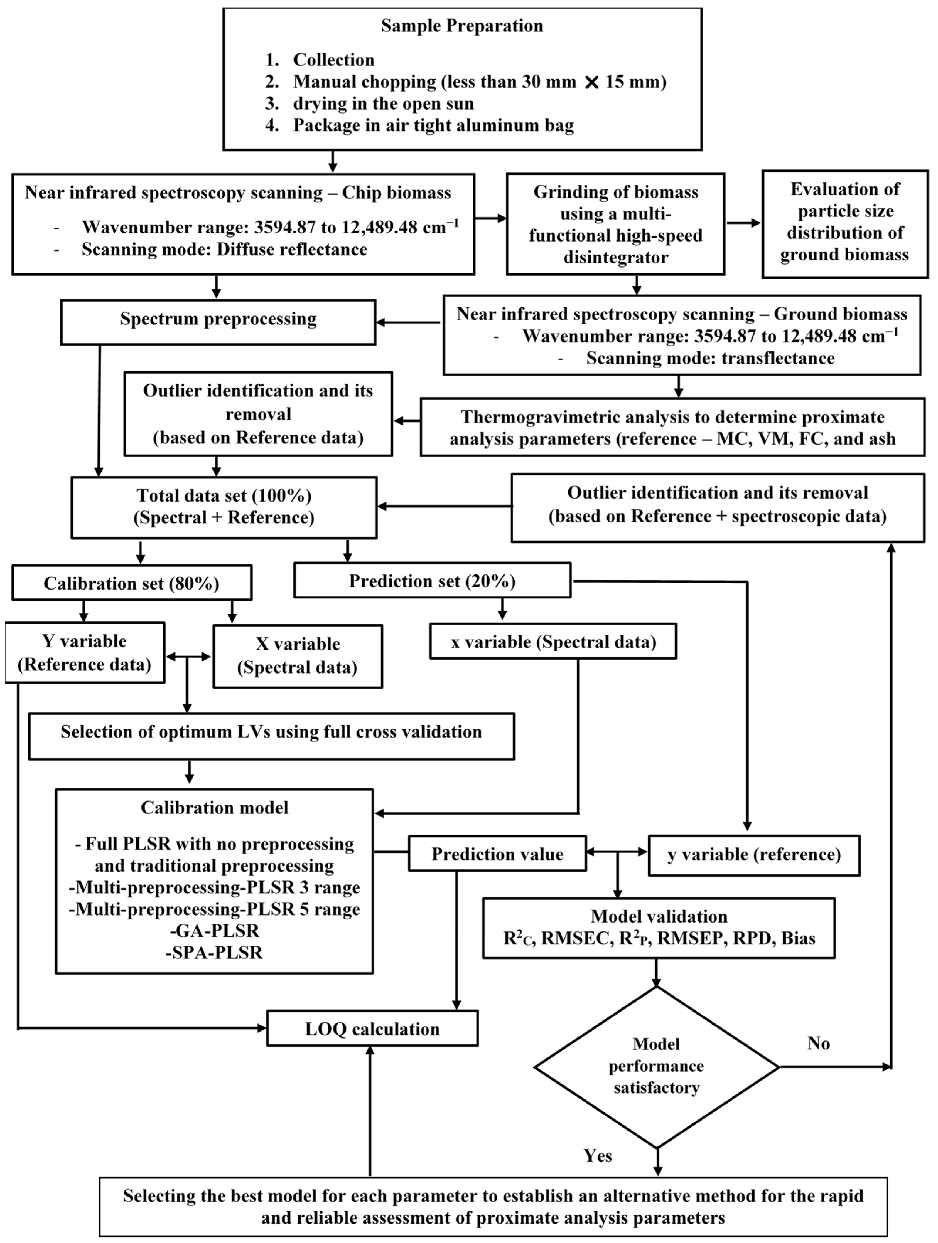
Figure 1 illustrates the overall research methodology employed to assess the proximate analysis parameters and select the best performance PLSR-based models using TGA (35−700 °C) and NIRS (3594.87−12,489.48 cm−1).

Figure 1.
Flowchart depicting the overall research methodology for the rapid assessment of biomass proximate analysis parameters using TGA, while using NIRS with PLSR as an alternative.
2.1. Sample Preparation
Ten different varieties of biomass samples were collected from various locations in Nepal. Wood samples included four fast-growing species: (1) Alnus nepalensis, (2) Pinux roxiburghii, (3) Bombax ceiba, and (4) Eucalyptus camaldulensis. Non-wood samples included five agricultural residues: (1) Zea mays (cob), (2) Zea mays (shell), (3) Zea mays (stover), (4) Oryza sativa, and (5) Saccharum officinarun and one fast-growing tree (6) Bombusa vulagris. These samples were manually chopped, dried under the open sun, and then transported to the laboratory for NIRS and TGA experiments to record the spectral data and proximate analysis data for the development of PLSR-based models [26].
2.2. FT-NIRS Scanning
In Figure 2a, chip biomass samples with dimensions less than 30 mm × 15 mm were scanned using an FT-NIR spectrometer (MPA, Bruker, Ettlingen, Germany) in diffuse reflectance and sphere macro sample rotating mode. The samples were fully filled into a quartz-bottom sample cup with a diameter of 90 mm and a height of 90 mm. They were then covered with aluminum sheet to prevent NIR leakage. Subsequently, the chip biomass samples were ground using a multifunctional high-speed disintegrator (WF−04, Thai grinder, Thailand). The ground biomass samples were scanned in a transflectance mode (Figure 2b). These samples were placed in glass vials with a diameter of 20 mm and a height of 40 mm.
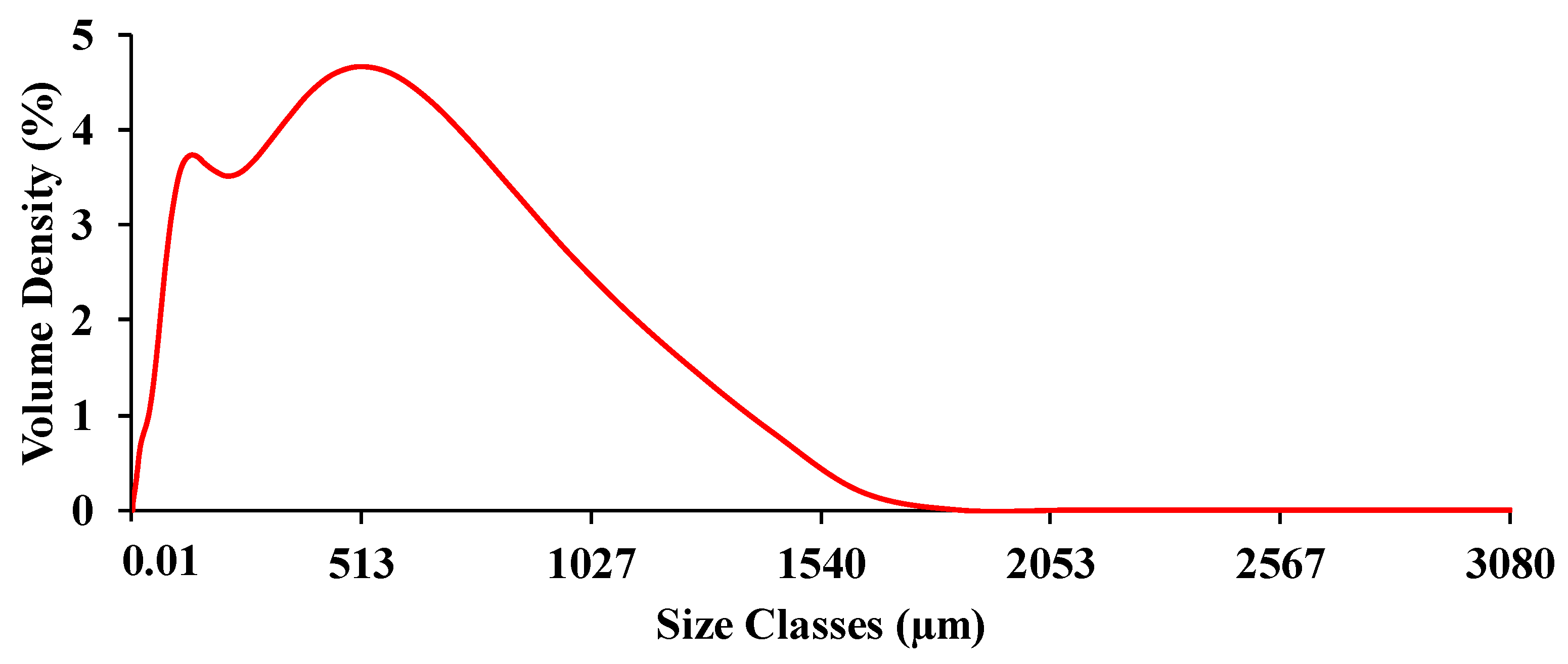
NIR scanning of both chip and ground biomass was performed twice without changing their positions under a controlled laboratory environment, maintaining a temperature of 25 ± 2 °C. For both forms of biomass samples, the spectrometer operated at a resolution of 16 cm−1, with a background scan time and sample scan time of 32 scans (average), logging absorbance data as Log (1/R) within a wavenumber range from 3594.87 to 12,489.48 cm−1. The average absorbance value was calculated and applied for model development. A gold plate scan was performed for every new scanning, and aluminum plates/handles were used to prevent possible NIR leakage. Figure 3 shows the raw spectra obtained by scanning the chip biomass and ground biomass using an FT-NIR spectrometer. The ground sample was randomly selected and its particle size distribution was assessed at the Scientific and Technological Research Equipment Center at Chulalongkorn University, Bangkok, Thailand, using the Mastersizer 3000 instrument (MAL1099267, Hydro MV). Figure 4 shows the representative particle size distribution of the ground biomass used in this research. The particle sizes range from 0.01 to 3080 µm, with an average particle size of 251.18 µm.

Figure 2.
FT-NIR spectrometer scanning of (a) chip biomass in diffuse reflectance and sphere macro sample rotating mode using a quartz-bottom sample cup, and (b) ground biomass in transflectance mode using a glass vial.
Figure 2.
FT-NIR spectrometer scanning of (a) chip biomass in diffuse reflectance and sphere macro sample rotating mode using a quartz-bottom sample cup, and (b) ground biomass in transflectance mode using a glass vial.
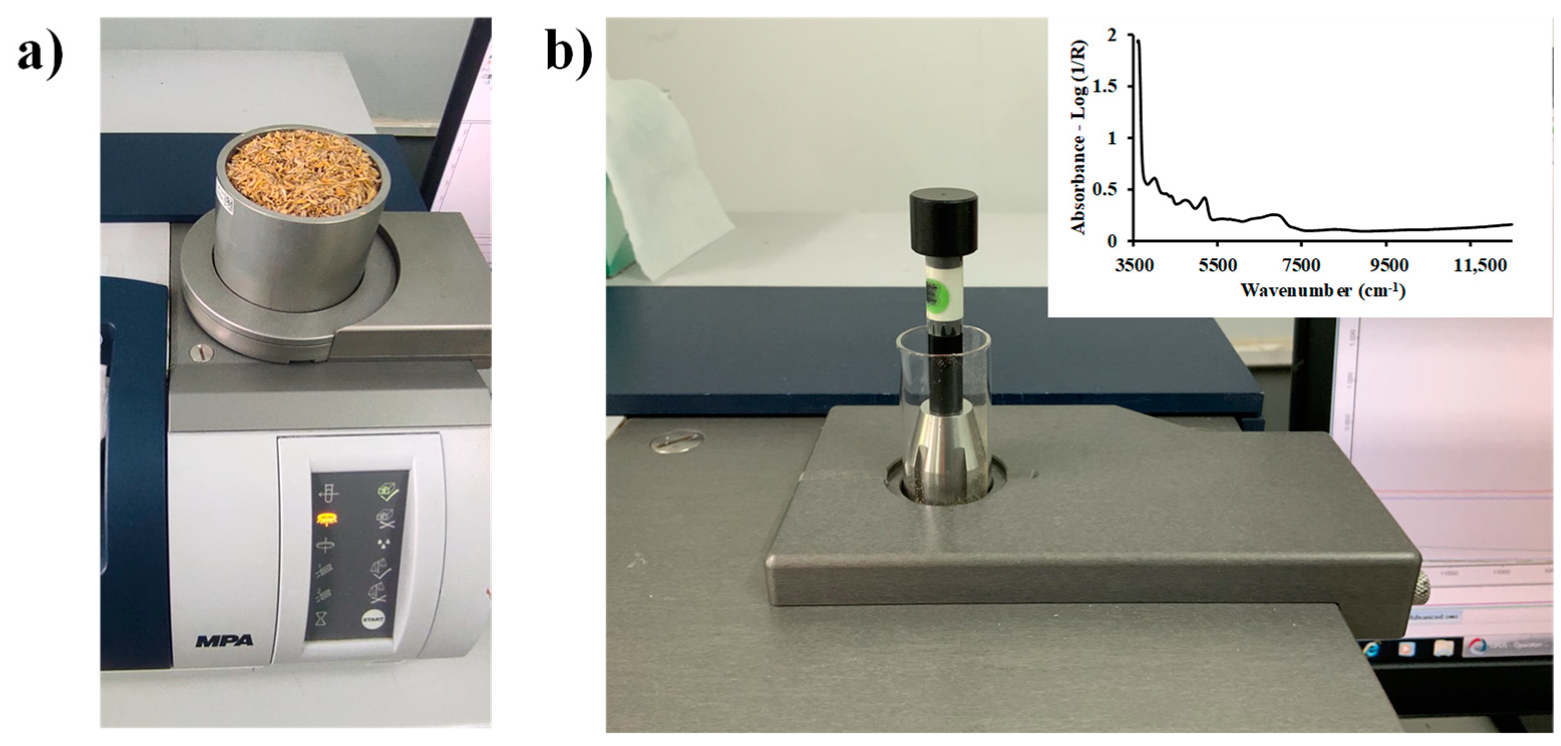

Figure 3.
Raw spectra of (a) chip biomass obtained from diffuse reflectance mode of FT-NIRS scanning and (b) ground biomass obtained from transflectance mode of FT-NIRS scanning across the entire wavenumber range from 3594.87 to 12,489.48 cm−1.
Figure 3.
Raw spectra of (a) chip biomass obtained from diffuse reflectance mode of FT-NIRS scanning and (b) ground biomass obtained from transflectance mode of FT-NIRS scanning across the entire wavenumber range from 3594.87 to 12,489.48 cm−1.

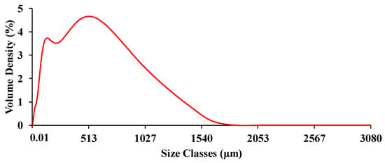
Figure 4.
Representative particle size distribution of the ground biomass ranging from 0.01 to 3080 µm.
Figure 4.
Representative particle size distribution of the ground biomass ranging from 0.01 to 3080 µm.
2.3. Reference Analysis (Proximate Analysis)
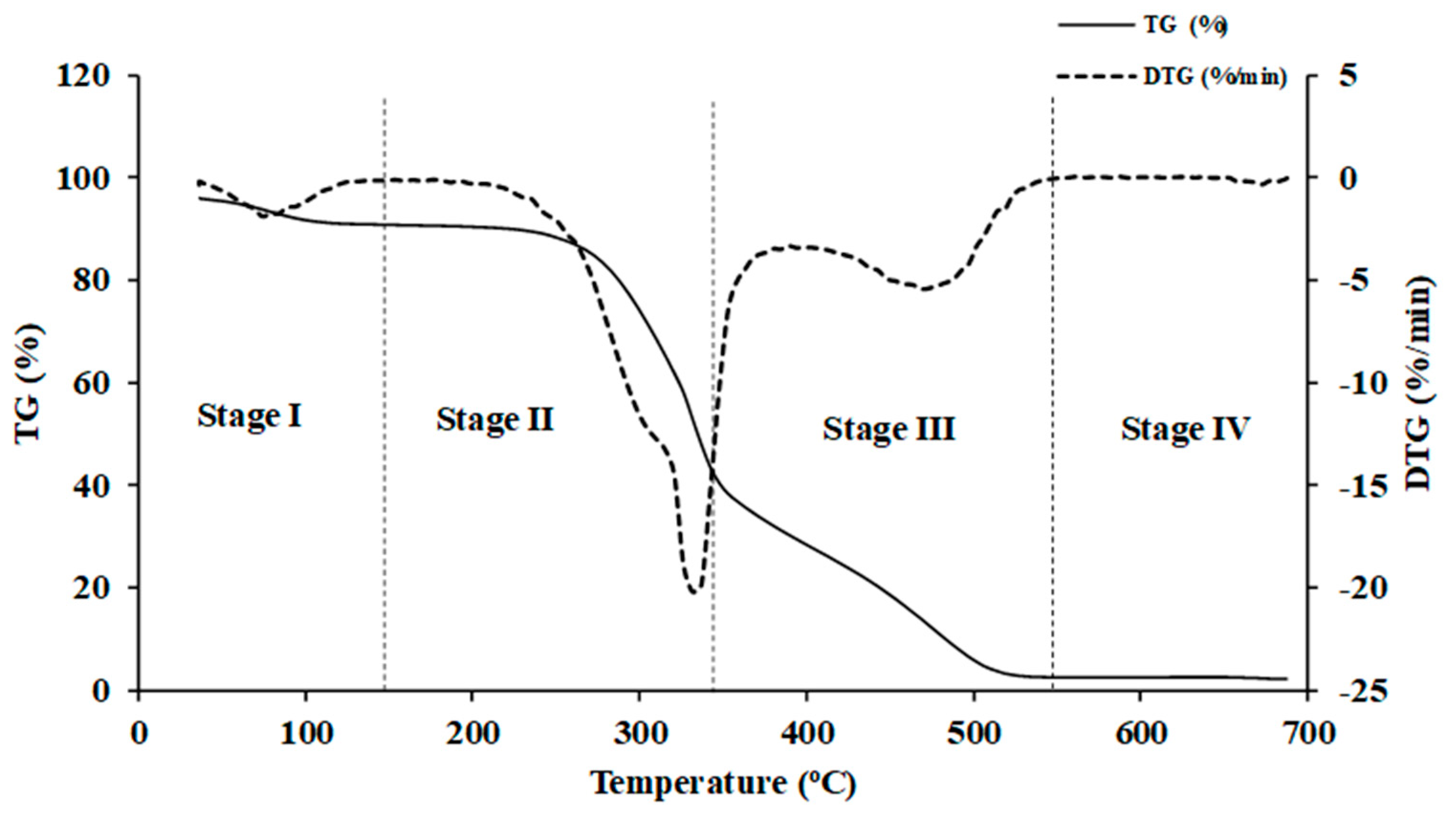
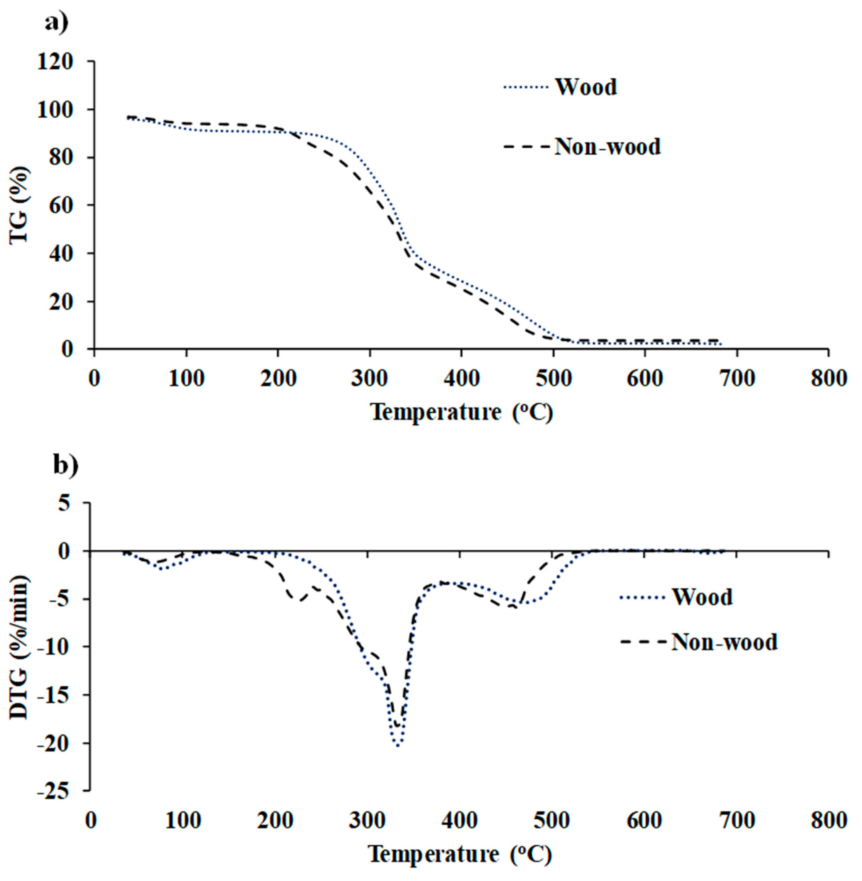
TGA (TG 209 F3 Tarsus, Netzsch, Germany) with a microbalance sensitivity of 0.1 µg resolution was employed for direct combustion in air atmosphere [30], i.e., O2 and N2 in 1:4 ratio, within a temperature range from 35 °C to 700 °C. A heat flow rate of 10 °C/min was utilized to record the mass loss of ground biomass sample of 6 ± 0.5 mg with respect to time or temperature. Prior to thermal biomass degradation, all samples were held isothermally at 35 °C for 10 min. N2 is used as a protective layer to create a stable and inert environment [31]. Proteus 6.0.0 (NETZSCH software, Germany) was used to generate TG and DTG curves. The TG and DTG curves were typical of the degradation process, which is generally divided into four significant stages: MC removal (<110—Stage I), release and combustion of VM (197–350 °C—Stage II), char combustion (360−600 °C—Stage III), and ash lifting (>600 °C—Stage IV) [24] (Figure 5). The representative TG and DTG curves of wood and non-wood biomass used in this study are shown in Figure 6a and Figure 6b, respectively.
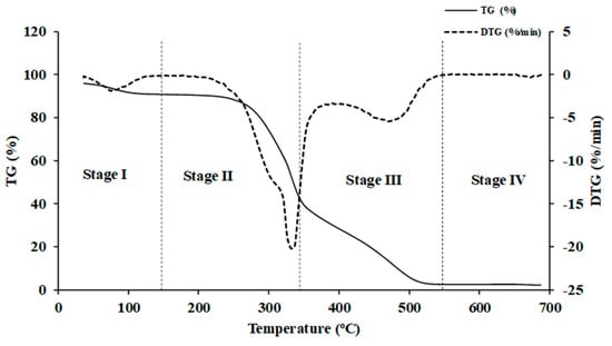
Figure 5.
The TG and DTG curves obtained from TGA analysis of Nepalese biomass.
Biomass is composed of cellulose, hemicellulose, and lignin [32]. As evident from Figure 6b, the combustion of lignocellulosic biomass exhibited two distinct major decomposition peaks. The first zone is within a temperature range of approximately 180–400 °C, where the rate of weight loss of biomass is at its maximum and the peak is prominently displayed. This range corresponds to the decomposition of cellulose and hemicellulose. During this phase, volatiles are released and subsequently ignited, resulting in the formation of char [33]. The second zone spans the temperature range from approximately 380 to 600 °C, where a broader peak was observed, associated with char oxidation [33]. In this stage, lignin assumes a key role as the primary contributor to biomass char formation. Beyond 535 °C, the decomposition primarily relates to inorganic matter, specifically the ash content.
In our reference test using the TGA (TG 209 F3 Tarsus, Netzsch, Germany), a small sample of approximately 6 mg was employed. Consequently, all the FT-NIRS scanned chip samples were ground to achieve a homogeneous mixture for obtaining the proximate parameters. It is important to note that this grinding method might slightly affect the measured constituent quantity in the sample, especially concerning MC. However, it is the only viable approach we have to compromise for estimating the MC in the chip sample using a small sample size for TG 209 F3 Tarsus.
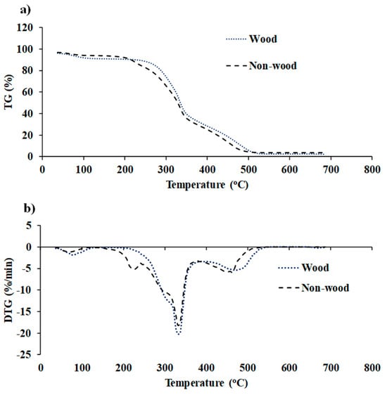
Figure 6.
(a) TG and (b) DTG profiles of fast-growing tree and agricultural residue biomass obtained using TGA within the temperature range from 35 to 700 °C with a heat flow rate of 10 °C/min.
Figure 6.
(a) TG and (b) DTG profiles of fast-growing tree and agricultural residue biomass obtained using TGA within the temperature range from 35 to 700 °C with a heat flow rate of 10 °C/min.
2.4. Outlier Identification
To achieve a high-performance predictive model, the identification and removal of outliers from the complete dataset is one of the most crucial procedures in NIR modeling. In this study, outliers were identified using two methods: one based solely on reference data and the other utilizing both reference and spectroscopic data.
Outlier for the reference data is calculated using the following equation:
where Xi is the measured reference value of sample i, and and SD denote the average and standard deviation of the measured values across all samples. If Equation (1) is satisfied for any sample i, the sample is considered an outlier and is removed from the complete dataset [26,34].
Following the removal of outliers based on Equation (1), the complete dataset was used to develop a model. If the model performance was deemed unsatisfactory, a further outlier identification process was undertaken using both reference and spectroscopic data. This method involved a full cross-validation using PLS regression on total dataset to identify outliers. A scatter plot was then created to compare the measured and predicted values. Outliers were carefully identified and subsequently removed if their behavior significantly deviated from the rest of the data points. This meticulous outlier detection process ensures the model accuracy by eliminating potential data anomalies that could impact the reliability of predictive results.
2.5. Spectral Preprocessing
Spectral preprocessing holds significant importance in NIR modeling to achieve high-performance predictions of the reference values using NIR spectral data. NIR raw spectral data often contain instrumental noise, baseline shift, over lapping peaks, scattering, and other errors [26]. Therefore, to enhance spectral features and extract the maximum relevant information, spectral preprocessing, which involves mathematical transformations, is vital prior to model development [35,36].
Prior to model development, raw spectra obtained from both chip and ground biomasses were subjected to ten different types of traditional spectral preprocessing, which include D1, D2, constant offset, SNV, MSC, min−max normalization, mean centering, vector normalization, D1 + MSC, and D1 + vector normalization. Additionally, the raw spectra were pretreated using MP techniques with a 5-range and 3-range to assess prediction performance within the same wavenumber range. In the MP 5-range technique, the entire spectral range is divided into five equal sections, while in the MP 3-range technique, the entire spectral range is divided into three different sections. It is preprocessed with different combination sets obtained from seven different preprocessing techniques, labeled as: 0 = empty (absorbance values = 0), 1 = raw spectra, 2 = SNV, 3 = MSC, 4 = D1, 5 = D2, and 6 = constant offset, covering the range from 3594.87 to 12,489.48 cm−1 [26]. These preprocessing steps could potentially improve and or even reduce the predictive accuracy [37] of proximate parameters for both chip and ground biomass.
The MATLAB−R2020b (MathWorks, Natick, MA, USA) with an in-house code was employed for conducting both traditional spectral preprocessing and multi-spectral preprocessing techniques.
2.6. Partial Least Squares Regression Model Development
After the identification and removal of outliers from the complete dataset, as shown in Figure 1, PLSR models were developed by manually splitting the total dataset which was run in descending order into a calibration set (80%) and a validation set (20%), ensuring that both sets include all varieties of biomass that have been considered. The calibration set is used to establish a mathematical model that correlates the reference data and spectral data of biomass samples. It includes the maximum and minimum reference values of the identified proximate parameters, ensuring the model was adequately trained to handle the entire spectrum of data. On the other hand, the prediction set employs the developed model to predict the properties of an unknown sample. In our study, Log (1/R) at different wavenumbers were used as independent variables in the regression model, and the regression coefficient represents the weight of each independent variable in series, where each weight was the change for a one-unit change in Log (1/R) at each wavenumber for prediction of a dependent variable.
The NIR spectra of each biomass sample contained multiple independent variables, resulting in collinearity issues, redundant information, and heightened computational complexity [20]. To tackle these challenges, uninformative wavelength variables, having either negligible or adverse impacts on model performance, need identification and elimination. In this study, two wavelength selection processes, GA and SPA, were employed to develop a PLSR model. The primary objective in choosing these wavelength selection methods is to improve predictive capacity, achieve higher model efficiency, and create simpler models that are more interpretable [38].
GA is an evolutionary optimization technique that mimics natural selection and genetic mechanisms to find optimal solutions, utilizing three key operators: selection, crossover, and mutation [39,40]. In feature wavelength selection, it begins by generating a population based on available features. Subsequently, the algorithm creates successive populations by selecting individuals based on their fitness level in the problem domain. These individuals undergo recombination through selection, crossover, and mutation across multiple generations, progressively eliminating redundant information from the chosen wavelengths [41]. The optimal member of the population becomes the selected feature.
SPA is a forward selection method that selects variables with minimal redundant information from the informative variable [38]. The variable selected by SPA has the greatest projection onto the orthogonal subspace of the previously selected variable [42]. In SPA, the initial phase involves projecting onto the columns of the spectral matrix, creating a candidate subset of variable with minimal collinearity. The subsequent step assesses these candidate subsets based on the RMSE values obtained from the validation set of the PLSR calibration. The final step involves removing uninformative variables through a variable elimination procedure that does not significantly compromise predictive ability [42,43,44].
In this study, five different PLSR-based models were constructed: Full-PLSR, MP PLSR 5-range, MP PLSR 3-range, GA-PLSR, and SPA-PLSR. These models were developed using an in-house code in MATLAB−R2020b (MathWorks, Natick, MA, USA) and their performances were subsequently compared.
The models were evaluated based on R2C, RMSEC, R2P, RMSEP, RPD, and bias. These parameters were calculated using Equations (2)–(5).
where y is the measured value, is the predicted value, i is the subscript used to indicate the number of the sample, is the mean of the measured value, N is the number of samples of the respective set, SD is the standard deviation of the measured values of the validation set, and n is the number of samples in the validation set.
The optimum model is selected based on higher R2C, R2P, and RPD values, as well as lower RMSEC and RMSEP values. In the case of similar performance, the model with fewer LVs is selected as an alternative method for rapid non-destructive evaluation of biomass proximate analysis parameters [26].
Williams et al. (2019) [45] and Zornoza et al. (2008) [46] guidelines have been followed for the interpretation of R2 and RPD values, respectively.
2.7. Limit of Quantification (LOQ)
The sensitivity of the selected high-performance PLSR model is a critical factor for reliably and accurately determining biomass proximate analysis parameters. To address this, the LOQ of the selected model is calculated, representing the minimum concentration of the analyte that can be detected and quantified with high sensitivity and reliability. There are different methods to calculate the LOQ, which is based on (1) visual evaluation, (2) signal-to-noise, and (3) the SD of the response to slope [47]. In this study, LOQ is calculated based on the SD of the response to slope method obtained from the calibration set. The LOQ is calculated using the following equation:
3. Results and Discussion
3.1. Spectral Preprocessing
Figure 7 displays the average pretreated spectrum obtained from the best-performing model for proximate analysis of chip or ground biomass. This model utilizes the following techniques: (a) MC with the second derivative from chip biomass, (b) VM with a MP combination set of 4, 3, 4, 6, and 0 from chip biomass, (c) FC with a constant offset from chip biomass, and (d) ash content with the first derivative from the ground biomass.
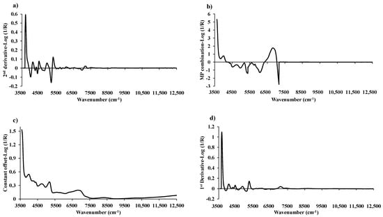
Figure 7.
The average pretreated spectra from the best performing model for: (a) MC with the second derivative, (b) VM with a multi-preprocessing combination set of 4, 4, 3, 2, and 0, (c) FC with a constant offset, and (d) ash content with the first derivative.
3.2. Reference Data
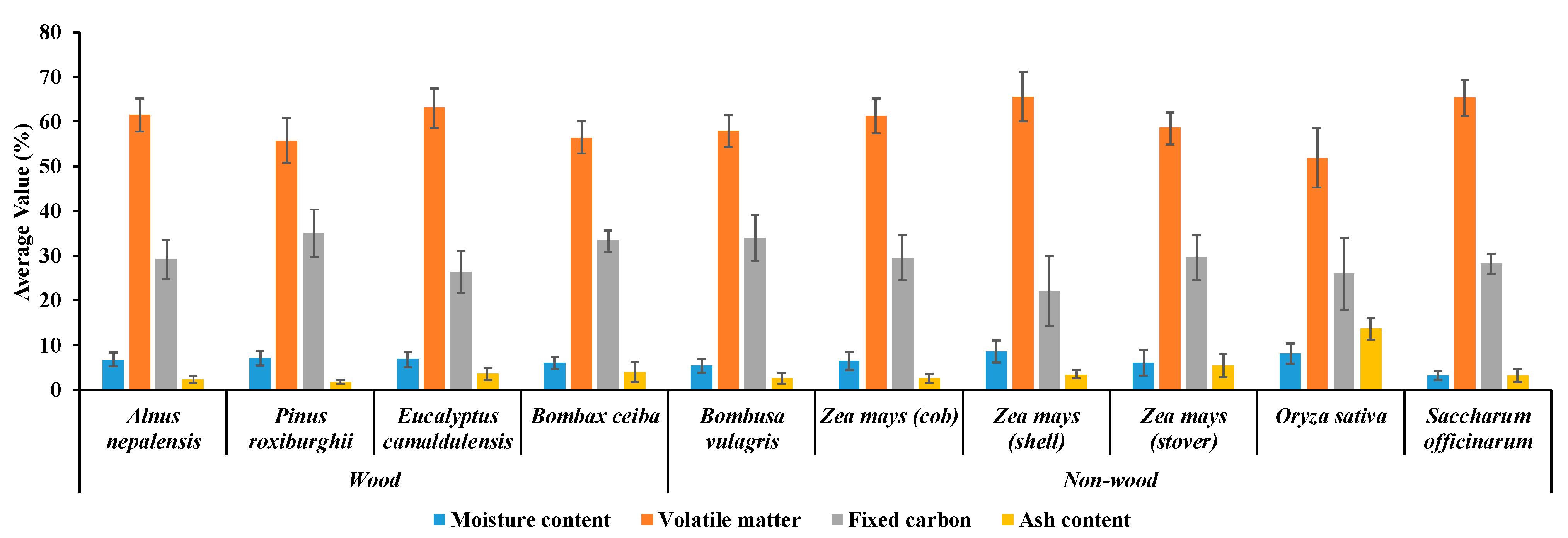
The proximate analysis data for ten different varieties of biomass, including four wood varieties of fast-growing trees and six non-wood varieties (five agricultural residues and one fast-growing tree) were obtained by analyzing the TG and DTG profiles obtained from TGA, as explained in Section 2.3. Figure 8 displays the comprehensive results of proximate analysis for biomass, encompassing MC, VM, FC, and ash content, all of which were obtained from TGA.
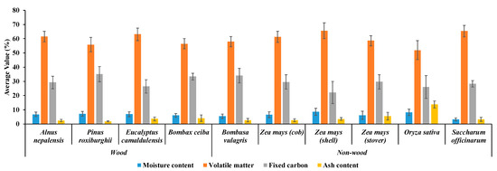
Figure 8.
Overall proximate analysis results of ten different biomass varieties, including four wood varieties of fast-growing trees and six non-wood varieties (five agricultural residues and one fast-growing tree) obtained from the TGA analysis.
Under the TGA, as explained in Section 2.3, the average MC, VM, FC, and ash content in the biomass samples were recorded as 6.47%, 58.99%, 31.63%, and 2.91%, respectively, and 6.55%, 60.57%, 27.17%, and 5.72%, respectively. Here, FC is calculated as:
FC (%) = 100 − MC (%) − VM (%) − ash (%),
The analysis revealed notable variations in MC, VM, FC, and ash content among the studied biomass varieties. The maximum MC of 8.61% and VM of 65.64% were recorded for Zea mays (shell), whereas the minimum MC of 3.19% was found in Saccharum officinarum, and the minimum VM of 51.96% was observed in Oryza sativa. Additionally, Pinus roxburghii exhibited the highest FC content at 35.11%, while Zea mays (shell) displayed the lowest FC content of 22.21%. Similarly, Oryza sativa had the maximum ash content of 13.72%, and Pinus roxburghii had the lowest ash content at 1.82%.
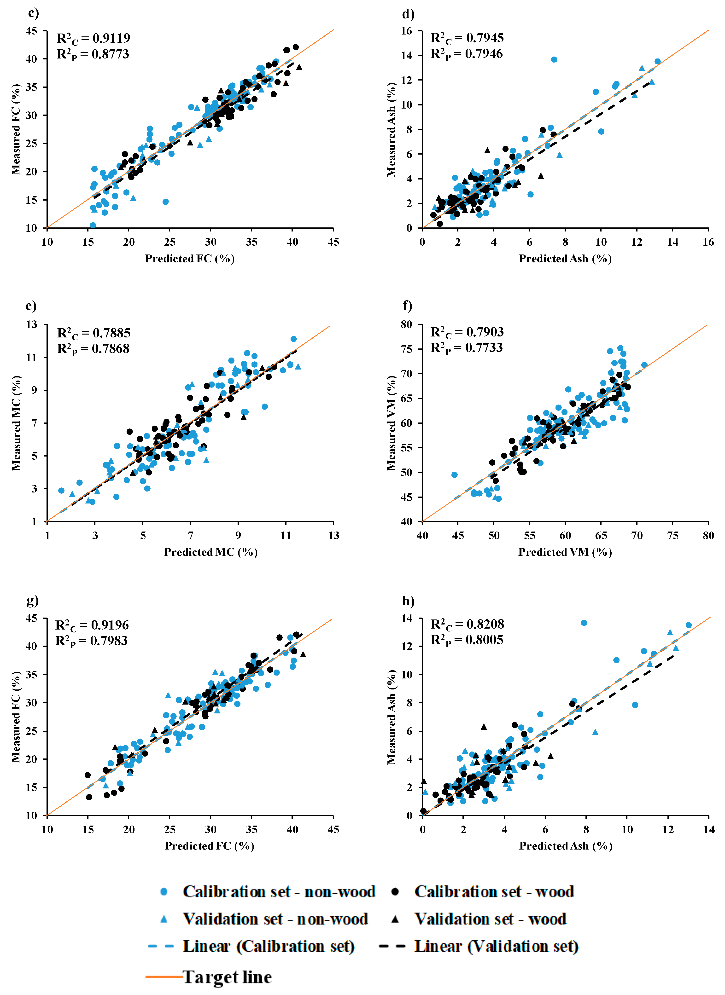
The MC, VM, FC, and ash content in fast-growing trees range from 3.50% to 10.39%, 48.31% to 69.74%, 18.95% to 42.05%, and 0.32% to 7.90%, respectively. For agricultural residues, the respective ranges are 2.21−12.21% (MC), 44.62−75.10% (VM), 10.40−35.83% (FC), and 0.88−17.59% (ash content). Interestingly, there seems to be an overlap in the ranges. This was confirmed by the data in Table 7 and scatter plots of the developed models shown in Figure 9, which indicated that the proximate parameter spans were wider when the wood and non-wood biomass of fast-growing trees and agricultural residue were combined for modeling.
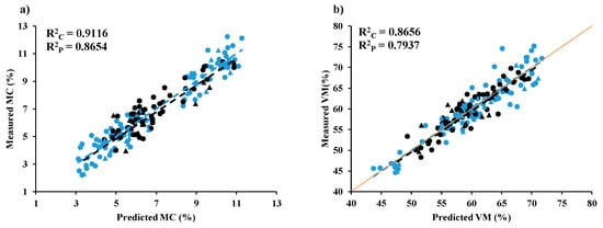
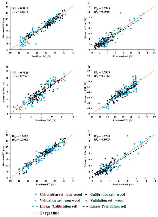
Figure 9.
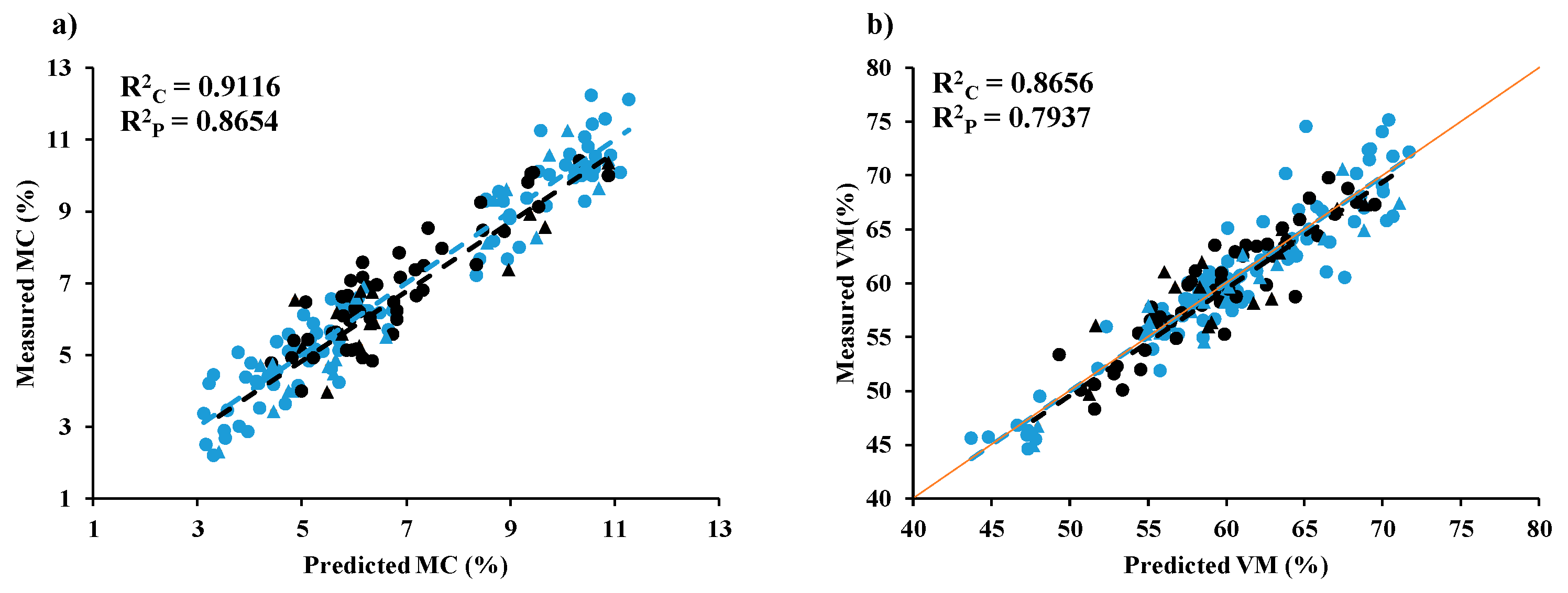
Measured versus predicted value in calibration set and validation set for chip biomass (a) MC, (b) VM, (c) FC, and (d) ash and for ground biomass (e) MC, (f) VM, (g) FC, and (h) ash.
The observed variations in MC among the biomass varieties are of significance. Despite all MC values falling below 10%, the notably higher MC in Zea mays (shell) highlights the necessity for effective drying procedures prior to utilizing it for energy purposes. Achieving an optimal MC could enhance the combustion efficiency of this biomass [48].
The diverse levels of VM content are indicative of differing combustion behaviors. Biomass with higher VM content tend to ignite more readily, making them favorable for certain combustion-based applications [10]. The presence of both high and low VM biomass, such as Zea mays (shell) and Oryza sativa, respectively, provides opportunities for specific use in different energy production processes.
The FC content is a crucial factor influencing combustion efficiency. Biomass with higher FC content generally possess better energy density and combustion characteristics [49]. In light of this, Pinus roxburghii contained notably higher FC content and is positioned as a promising biomass for energy production, particularly in scenarios where concerns related to ash generation and deposition need to be minimized.
Furthermore, ash content is a critical consideration in combustion processes. Lower ash content, such as in Pinus roxburghii, can alleviate operational challenges associated with ash accumulation. Conversely, Oryza sativa had higher ash content and might require careful management or additional treatment to mitigate potential issues during combustion.
3.3. Prediction of Proximate Analysis Data
Table 1 shows the statistical summary data for the proximate parameters: MC, VM, FC, and ash. These parameters were employed in both the calibration and validation sets to develop a PLSR-based model for both chipped and ground biomass, using the full wavenumber range from 3594.87 to 12,489.48 cm−1 to assess proximate analysis parameters. Table 2 shows the details of outliers identified in chip and ground biomass, which were subsequently removed from the total dataset for PLSR model development. Table 3 shows PLSR modeling results for chipped biomass, and Table 4 shows the results for ground biomass, with the bolded model showing the best performance in each parameter.
3.3.1. Moisture Content (%)
Table 2 shows the count of outliers identified for MC in chip (based on reference data) and ground biomass (based on both reference and spectroscopic data). After the removal of these outliers, PLSR-based models were developed to evaluate the percentage of MC in chip and ground biomass. The model performance was assessed across various preprocessing techniques, and the best-performing model, selected as the optimal choice among five different types of PLSR-based models, was highlighted in bold in both Table 3 and Table 4.

Table 1.
Statistical data of the proximate analysis parameters of the chip and ground biomass used in the PLSR model development.
Table 1.
Statistical data of the proximate analysis parameters of the chip and ground biomass used in the PLSR model development.
| Category | Parameters (%) | NT | Calibration Set | Validation Set | ||||||||
|---|---|---|---|---|---|---|---|---|---|---|---|---|
| NC | Max | Min | Mean | SD | NP | Max | Min | Mean | SD | |||
| Chip | MC | 173 | 138 | 12.21 | 2.21 | 6.83 | 2.37 | 35 | 11.24 | 2.29 | 6.81 | 2.35 |
| VM | 173 | 138 | 75.10 | 44.62 | 60.12 | 6.39 | 35 | 70.59 | 44.84 | 59.42 | 5.52 | |
| FC | 173 | 138 | 42.05 | 10.40 | 28.91 | 7.06 | 35 | 38.55 | 13.23 | 28.32 | 6.15 | |
| Ash | 162 | 130 | 13.64 | 0.32 | 3.53 | 2.34 | 32 | 12.97 | 1.37 | 4.17 | 2.90 | |
| Ground | MC | 157 | 126 | 12.10 | 2.21 | 6.72 | 2.26 | 31 | 10.42 | 2.29 | 6.49 | 2.37 |
| VM | 174 | 139 | 75.10 | 44.62 | 60.11 | 6.37 | 35 | 70.59 | 44.84 | 59.42 | 5.52 | |
| FC | 152 | 122 | 42.05 | 13.23 | 29.08 | 6.71 | 30 | 38.55 | 15.33 | 29.11 | 5.63 | |
| Ash | 163 | 130 | 13.64 | 0.32 | 3.56 | 2.35 | 33 | 12.97 | 1.37 | 4.15 | 2.86 | |

Table 2.
Details on the number of identified outliers in chip and ground biomass evaluated before the development of the PLSR model.
Table 2.
Details on the number of identified outliers in chip and ground biomass evaluated before the development of the PLSR model.
| Proximate Parameter (%) | Chip Biomass | Ground Biomass | ||
|---|---|---|---|---|
| Total Number of Sample | Ouliers | Total Number of Sample | Ouliers | |
| MC | 173 | 0 | 174 | 17 |
| VM | 173 | 0 | 174 | 0 |
| FC | 173 | 0 | 174 | 22 |
| Ash | 173 | 11 | 174 | 11 |
In Figure 9a, the scatter plot displays the measured and predicted MC (%) values for wood and non-wood samples in both the calibration and validation sets, using GA-PLSR. The best performance was achieved with GA-PLSR utilizing 10 LVs, D2 spectral pretreatment, and 57 important wavenumbers (Table 3). A notable 2.82% improvement in explained variance from Full-PLRS (R2P = 0.8417) to GA-PLSR (R2P = 0.8654) was observed. This improvement can be attributed to GA-PLSR efficient feature selection and model parameter optimizations, resulting in a more accurate and precise predictive model. The increased explained variance indicates a stronger correlation between the spectral data (independent variable) and the reference data (dependent variable), ultimately enhancing the predictive capabilities of the model.
Similarly, Figure 9e displays a scatter plot depicting the measured and predicted MC (%) of ground biomass using mean centering. The Full-PLSR model, employing 12 LVs and mean centering as spectral preprocessing, exhibited the best performance (Table 4). An enhancement of 19.72% in explained variance was observed, transitioning from Full-PLSR using raw spectra (R2P = 0.6752) to Full-PLSR employing mean centering (R2P = 0.7868). Furthermore, the use of mean centering indicates that the model accuracy can be improved by removing baseline shifts, aligning spectral data around a common central point, and mitigating systematic variations caused by instrumental effects such as intensity fluctuations.

Table 3.
Results of the PLS regression-based model for the proximate analysis (%) of chip biomass, with the bolded model showing the best performance.
Table 3.
Results of the PLS regression-based model for the proximate analysis (%) of chip biomass, with the bolded model showing the best performance.
| Parameter | Algorithm | Preprocessing | LVs | Calibration Set | Validation Set | ||||
|---|---|---|---|---|---|---|---|---|---|
| R2c | RMSEC (%) | R2p | RMSEP (%) | RPD | Bias (%) | ||||
| MC | Full-PLSR | D1 | 14 | 0.9498 | 0.53 | 0.8417 | 0.92 | 2.5 | −0.14 |
| SPA-PLSR | Constant offset (SW: 100) | 12 | 0.8587 | 0.89 | 0.8281 | 0.96 | 2.4 | −0.02 | |
| GA-PLSR | D2 (SW: 57) | 10 | 0.9116 | 0.70 | 0.8654 | 0.85 | 2.9 | −0.25 | |
| MP-PLSR-5 range | Combination set: 4, 3, 4, 6, 0 | 13 | 0.9280 | 0.63 | 0.8260 | 0.97 | 2.4 | −0.13 | |
| MP-PLSR-3 range | Combination set: 4, 6, 0 | 11 | 0.9194 | 0.67 | 0.8386 | 0.93 | 2.5 | −0.13 | |
| VM | Full-PLSR | Constant offset | 15 | 0.8719 | 2.28 | 0.7725 | 2.60 | 2.1 | −0.56 |
| SPA-PLSR | Mean Centering (SW: 971) | 12 | 0.8345 | 2.59 | 0.7720 | 2.60 | 2.2 | −0.61 | |
| GA-PLSR | D1 (SW: 423) | 9 | 0.8460 | 2.50 | 0.7801 | 2.55 | 2.2 | −0.44 | |
| MP-PLSR-5 range | Combination set: 4, 4, 3, 2, 0 | 15 | 0.8656 | 2.33 | 0.7937 | 2.47 | 2.2 | −0.48 | |
| MP-PLSR-3 range | Combination set: 4, 4, 0 | 9 | 0.8368 | 2.57 | 0.7504 | 2.72 | 2.0 | −0.46 | |
| FC | Full-PLSR | Constant offset | 15 | 0.9119 | 2.09 | 0.8773 | 2.12 | 3.0 | −0.64 |
| SPA-PLSR | Constant offset (SW: 711) | 12 | 0.8831 | 2.40 | 0.8759 | 2.14 | 3.0 | −0.74 | |
| GA-PLSR | Constant offset (SW: 412) | 15 | 0.9081 | 2.13 | 0.8762 | 2.13 | 3.0 | −0.72 | |
| MP-PLSR-5 range | Combination set: 4, 4, 4 | 10 | 0.9060 | 2.16 | 0.8432 | 2.40 | 2.7 | −0.77 | |
| MP-PLSR-3 range | Combination set: 5, 1, 6, 6, 6 | 13 | 0.9008 | 2.21 | 0.8680 | 2.20 | 2.9 | −0.66 | |
| Ash | Full-PLSR | D2 | 12 | 0.8074 | 1.02 | 0.7596 | 1.40 | 2.1 | −0.20 |
| SPA-PLSR | D1 (SW: 458) | 14 | 0.7554 | 1.15 | 0.7544 | 1.42 | 2.0 | −0.21 | |
| GA-PLSR | D1 (SW: 175) | 13 | 0.7805 | 1.09 | 0.7638 | 1.39 | 2.1 | −0.17 | |
| MP-PLSR-5 range | Combination set: 5, 6, 5, 0, 0 | 15 | 0.7645 | 1.13 | 0.7648 | 1.39 | 2.1 | −0.27 | |
| MP-PLSR-3 range | Combination set: 5, 4, 4 | 13 | 0.7945 | 1.06 | 0.7946 | 1.29 | 2.2 | −0.22 | |
Figure 10 displays the average absorbance spectra after undergoing D2 pretreatment, with 57 significant wavenumbers highlighted in red to emphasize their importance as identified through GA. The highest peaks were observed at 3722, 4525, 5000, and 5285 cm−1, all of which could have the potential to enhance the model performance derived from GA-PLSR for MC (%).
Similarly, Figure 11 illustrates the regression coefficients for the MC (%) of ground biomass using Full-PLSR with spectra preprocessed through mean centering. Significant peaks were identified at 3650, 4902, 7042, and 8163 cm−1, which could have a substantial impact on enhancing the model performance.

Table 4.
Results of the PLS regression-based model for the proximate analysis (%) of ground biomass, with the bolded model showing the best performance.
Table 4.
Results of the PLS regression-based model for the proximate analysis (%) of ground biomass, with the bolded model showing the best performance.
| Parameter | Algorithm | Preprocessing | LVs | Calibration Set | Validation Set | ||||
|---|---|---|---|---|---|---|---|---|---|
| R2c | RMSEC (%) | R2p | RMSEP (%) | RPD | Bias (%) | ||||
| MC | Full-PLSR | Mean Centering | 12 | 0.7885 | 1.03 | 0.7868 | 1.08 | 2.2 | 0.01 |
| SPA-PLSR | D1 + vector normalization (SW: 125) | 15 | 0.7754 | 1.07 | 0.7624 | 1.14 | 2.1 | 0.05 | |
| GA-PLSR | Constant offset (SW: 925) | 13 | 0.8083 | 0.98 | 0.7582 | 1.15 | 2.0 | −0.07 | |
| MP-PLSR-5 range | Combination set: 5, 4, 0, 4, 6 | 12 | 0.8338 | 0.92 | 0.7727 | 1.11 | 2.1 | 0.18 | |
| MP-PLSR-3 range | Combination set: 4, 4, 1 | 15 | 0.8854 | 0.76 | 0.7123 | 1.25 | 1.9 | 0.00 | |
| VM | Full-PLSR | SNV | 15 | 0.8363 | 2.57 | 0.7557 | 2.69 | 2.2 | −1.17 |
| SPA-PLSR | SNV (SW: 931) | 14 | 0.8213 | 2.68 | 0.7513 | 2.71 | 2.2 | −1.18 | |
| GA-PLSR | SNV (SW: 383) | 9 | 0.7382 | 3.25 | 0.7305 | 2.83 | 2.1 | −1.24 | |
| MP-PLSR-5 range | Combination set: 3, 5, 4, 5, 0 | 9 | 0.7903 | 2.91 | 0.7733 | 2.59 | 2.3 | −1.09 | |
| MP-PLSR-3 range | Combination set: 4, 2, 6 | 14 | 0.8245 | 2.66 | 0.7323 | 2.82 | 2.2 | −1.32 | |
| FC | Full-PLSR | D1 | 14 | 0.9196 | 1.90 | 0.7983 | 2.49 | 2.3 | 0.67 |
| SPA-PLSR | D1 (SW: 945) | 14 | 0.9139 | 1.96 | 0.7965 | 2.50 | 2.3 | 0.64 | |
| GA-PLSR | D1 + vector normalization (SW: 74) | 14 | 0.8465 | 2.62 | 0.7034 | 3.02 | 1.9 | 0.85 | |
| MP-PLSR-5 range | Combination set: 1, 4, 1, 4, 1 | 13 | 0.8743 | 2.37 | 0.7932 | 2.52 | 2.2 | 0.19 | |
| MP-PLSR-3 range | Combination set: 6, 5, 1 | 12 | 0.8217 | 2.82 | 0.7732 | 2.64 | 2.1 | 0.20 | |
| Ash | Full-PLSR | D1 | 13 | 0.8208 | 0.99 | 0.8005 | 1.26 | 2.2 | 0.04 |
| SPA-PLSR | D1 (SW: 1089) | 13 | 0.8216 | 0.99 | 0.8005 | 1.26 | 2.2 | 0.03 | |
| GA-PLSR | SNV (SW: 112) | 15 | 0.7973 | 1.05 | 0.7834 | 1.31 | 2.2 | 0.20 | |
| MP-PLSR-5 range | Combination set: 4, 6, 3, 5, 3 | 15 | 0.8818 | 0.81 | 0.7971 | 1.27 | 2.2 | 0.14 | |
| MP-PLSR-3 range | Combination set: 4, 6, 2 | 11 | 0.7765 | 1.11 | 0.7705 | 1.35 | 2.1 | 0.07 | |
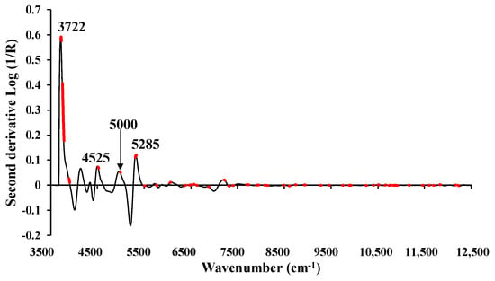
Figure 10.
The average absorbance value of MC (%) of chip biomass obtained using second derivative preprocessing with a selection of important wavenumbers obtained from GA.
Figure 10.
The average absorbance value of MC (%) of chip biomass obtained using second derivative preprocessing with a selection of important wavenumbers obtained from GA.
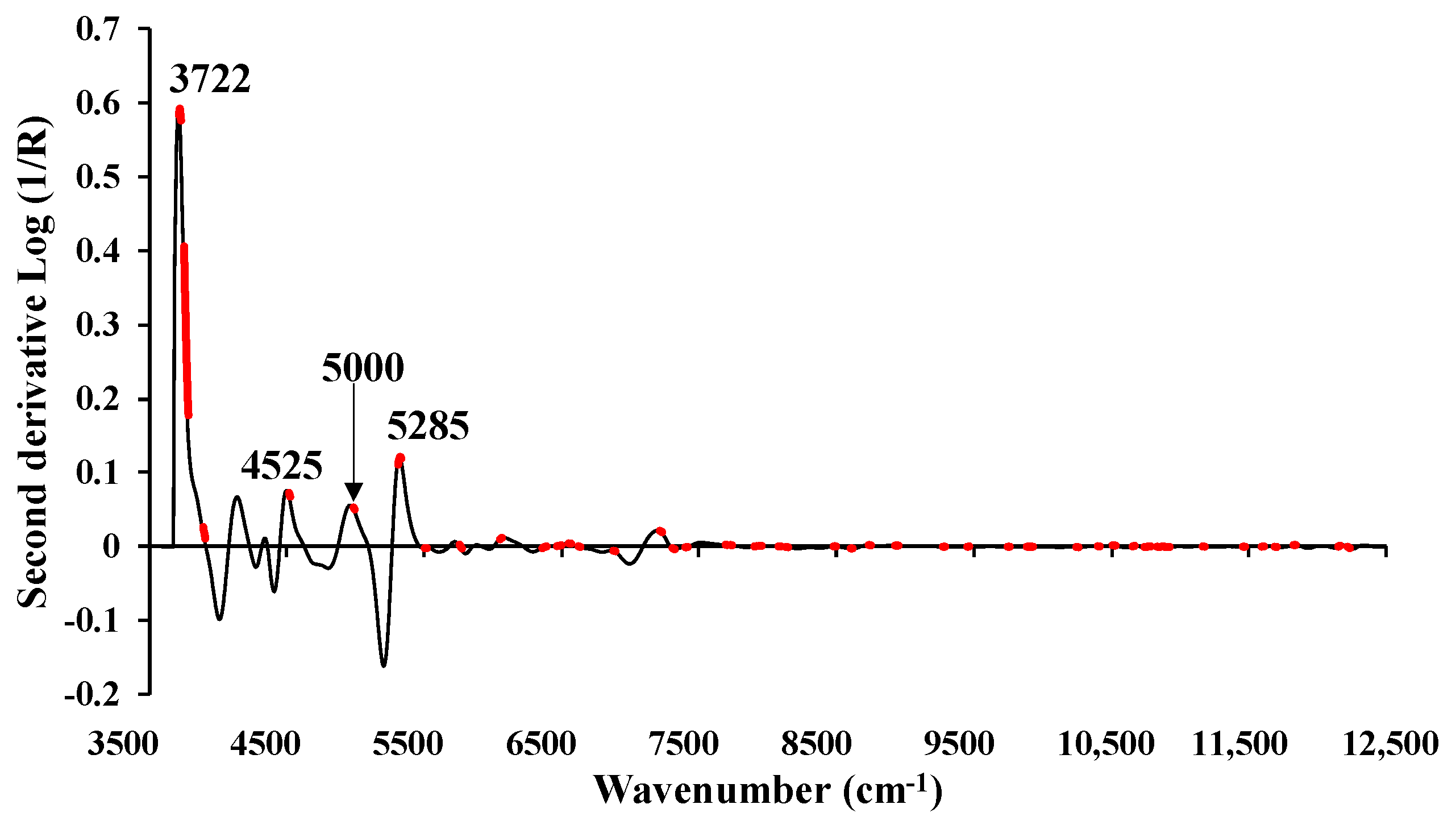

Figure 11.
The regression coefficient for the MC (%) of ground biomass using the Full-PLSR with spectral preprocessing of mean centering.
Figure 11.
The regression coefficient for the MC (%) of ground biomass using the Full-PLSR with spectral preprocessing of mean centering.
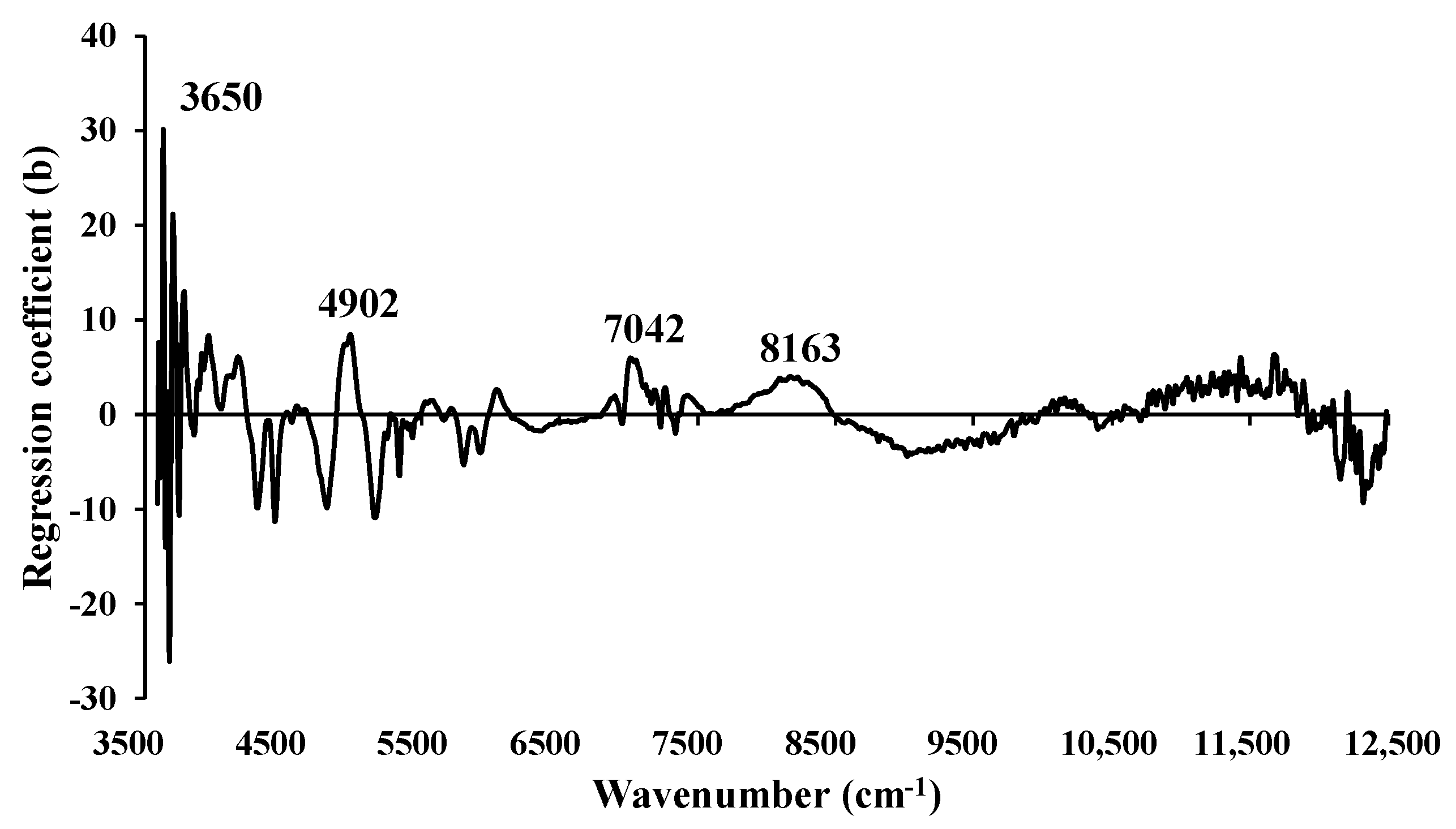
Table 5 [50] tabulates the bond vibration and corresponding functional group, spectra-structure, and material type which were found in the featured wavelength plot and regression coefficient plots by near-infrared spectroscopy analysis of chip and ground biomass for proximate analysis parameters which are derived from the best performing models in this study. Figure 10, Figure 12, Figure 14 and Figure 16 are for chip models and Figure 11, Figure 13, Figure 15 and Figure 17 are for ground biomass models for MC, VM, FC, and ash, respectively.
3.3.2. Volatile Matter (%)
For VM, no outliers were identified in either chip or ground biomass (Table 3). Therefore, models were developed as explained in Section 2.6. For both chip and ground biomass, the PLSR model developed using the spectral MP 5-range methods yielded the highest performance.
For chip biomass, the best result was obtained with a spectral preprocessing combination set of 4, 4, 3, 2, 0, i.e., D1, D1, MSC, SNV, and zero, respectively, from the range 3625.72–12,489.48 cm−1, which is equally divided into five sections. Figure 9b displays the scatter plot of measured versus predicted percentages of VM in wood and non-wood samples for the calibration and validation sets. When compared with the best model performance (Table 3) obtained from Full-PLSR using a constant offset (R2P of 0.7725), the MP 5-range PLSR method resulted in a 2.7443% improvement in explained variance.

Table 5.
The dominant peaks on the regression coefficient plot obtained from the best-performing PLSR-based model.
Table 5.
The dominant peaks on the regression coefficient plot obtained from the best-performing PLSR-based model.
| Proximate Parameter | Biomass Type | Peak Wavelength (cm−1) | Functional Group | Spectra-Structure | Material Type | Reference |
|---|---|---|---|---|---|---|
| MC | Chip | 3722 | C−H aromatic C−H (aryl) | C−H aryl | [50] | |
| 4525 | N−H ammonia in water | N−H (3ν) for NH3 (ammonia) in water | Ammonia in water | |||
| 5000 | N−H ammonia in water | Ammonia | ||||
| 5285 | O−H hydrogen bonding between water and expoxed polyvinyl alcohol OH | Water and polyvinyl alcohol OH | ||||
| Ground | 3650 | O−H from primary alcohols as (−CH−OH) | O−H (ν)(−CH2−OH), Primary alcohols | Primary alcohols | ||
| 4902 | N−H combination band from urea | N−H for primary amides | Urea | |||
| 7042 | O−H aromatic (ArO−H) | O−H (2ν), .O−H | Hydrocarbons, aromatic | |||
| 8163 | C−H secondary or tertiary carbon (.CH) | C−H (3ν), .C−H | Hydrocarbons, aliphatic | |||
| VM | Chip | 4019 | C−H/C−C (.C−H and .C−C) | C−H stretching and C−C stretching combination | Cellulose | [50] |
| 5495 | O−H/C−H combination | O−H stretching and C−O stretching combination | Cellulose | |||
| 5865 | C−H methyl (.CH3) | C−H methyl (.CH3) | Hydrocarbons, methyl | |||
| 6944 | C−H methylene (.CH2) | C−H combination, .C−H2 | Hydrocarbons, aliphatic | |||
| Ground | 3693 | C−H aromatic C−H (aryl) | C−H aryl | |||
| 4505 | N−H combination band from urea (NH2−C=O−NH2) | N-H combination | N−H from urea | |||
| 5200 | O−H assigned to molecular water [O−H (O−H and HOH)] | O−H stretching and HOH deformation combination | O−H molecular water | |||
| 5735 | C−H methyl C−H, aromatic associated (ArCH3) | C−H mythyl, aromatic (ArCH3) | Aromatic (ArCH3) | |||
| 5952 | C−H aromatic (ArCH) | C−H (2ν), aromatic C−H | Hydrocarbons, aromatic | |||
| FC | Chip | 3722 | C−H aromatic C−H (aryl) | C−H aryl | [50] | |
| 4405 | O−H/C−H cellulose (.OH and .C−O) | O−H stretching and C−O stretching combination | Cellulose | |||
| 5952 | C−H aromatic (ArCH) | C−H (2ν), aromatic C−H | Hydrocarbons, aromatic | |||
| 8754 | C−H aromatic (ArCH) | C−H (3ν), aromatic C−H | Hydrocarbons, aromatic | |||
| Ground | 3733 | C−H aromatic C−H (aryl) | C−H aryl | |||
| 4099 | C−H aromatic C−H (aryl) | C−H aryl | ||||
| 5903 | C−H methyl C−H, (CH3) (Asymmetric) | C−H (2ν), methyl | Hydrocarbons, aliphatic | |||
| 11,655 | C−H aromatic (ArCH) | C−H (4ν), aromatic C−H | Hydrocarbons, aromatic | |||
| Ash | Chip | 4019 | C−H/C−C (C−H and C−C) | C−H stretching and C−C stretching combination | Cellulose | [50] |
| 5285 | O−H hydrogen bonding between water and expoxed polyvinyl alcohol OH | Water and polyvinyl alcohol OH | ||||
| 11,655 | C−H aromatic (ArCH) | C−H (4ν), aromatic C−H | Hydrocarbons, aromatic | |||
| 12,048 | C−H methylene C−H, associated with linear aliphatic R(CH2)NR | C−H combination | Hydrocarbons, aliphatic | |||
| Ground | 4505 | N−H combination band from urea (NH2−C=O−NH2) | N−H combination | N−H from urea | ||
| 5285 | O−H hydrogen bonding between water and expoxed polyvinyl alcohol OH | Water and polyvinyl alcohol OH | ||||
| 11,655 | C−H aromatic (ArCH) | C−H (4ν), aromatic C−H | Hydrocarbons, aromatic | |||
| 12,300 | C−H methylene C−H, associated with branched aliphatic RC(CH3)3 | C−H combination | Hydrocarbons, aliphatic |
ν: Fundamental stretching vibrational absorption band, 2ν: First overtone of fundamental stretching band, 3ν: Second overtone of fundamental stretching band, 4ν: Third overtone of fundamental stretching band.
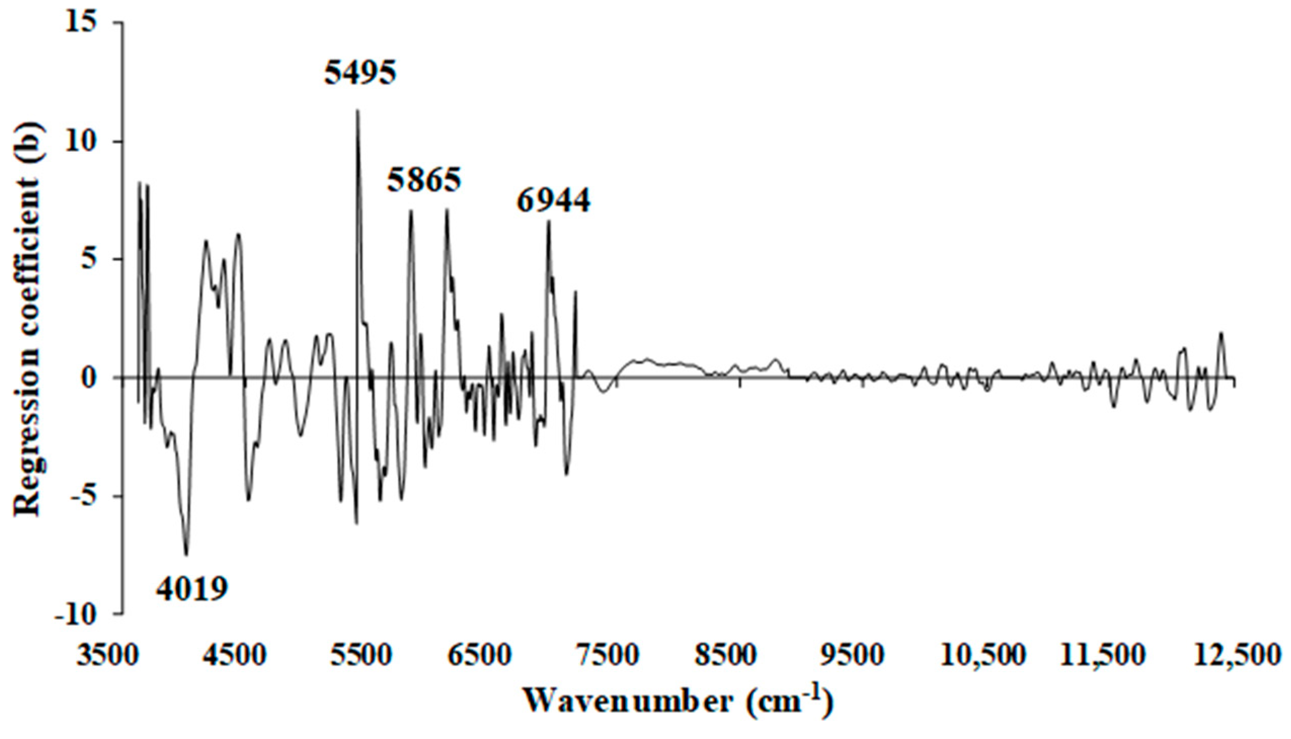
Figure 12 shows the regression coefficient plot for the % of VM in chip biomass, derived from the MP PLSR 5-range method. The important peaks were observed at the wavenumbers 4019, 5495, 5865, and 6944 cm−1 (Table 5), which could significantly influence the improved performance of the selected model.
Figure 12.
Regression coefficient for the % of VM in chip biomass using the MP PLSR 5-range method with a spectral multi-preprocessing combination set of 4, 4, 3, 2, and 0.
Figure 12.
Regression coefficient for the % of VM in chip biomass using the MP PLSR 5-range method with a spectral multi-preprocessing combination set of 4, 4, 3, 2, and 0.
The model achieved its best performance for VM (%) in the ground biomass with a spectral preprocessing combination set of 3, 5, 4, 5, and 0, i.e., MSC, D2, D1, D2, and zero absorbance—in the range of 3625.72−12,489.48 cm−1, equally divided into five sections. This MP PLSR 5-range resulted in an R2P of 0.7733 (Table 4), signifying a notable improvement of 2.3290% compared to Full-PLSR (R2P = 0.7557).
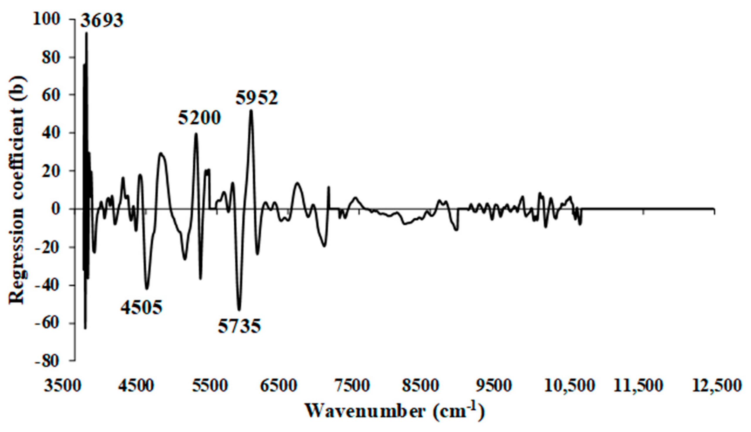
As shown in Figure 13, significant peaks were observed at wavenumbers 3693, 4505, 5200, 5735, and 5952 cm−1 (Table 5), all of which could exert a notable influence on the enhanced performance of the model using the MP PLSR 5-range method. Within the wavenumber range between 10,722.9 and 12,489.48 cm−1, the regression coefficient was observed to be zero. This suggests that the range lacks relevant spectral information for predicting VM in ground biomass.
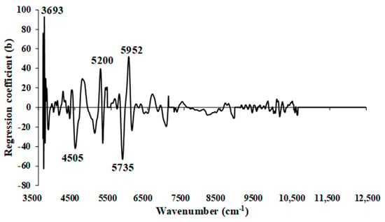
Figure 13.
Regression coefficient for the % of VM in ground biomass using the MP PLSR 5-range method with a spectral multi-preprocessing combination set of 3, 5, 4, 5, and 0.
Figure 13.
Regression coefficient for the % of VM in ground biomass using the MP PLSR 5-range method with a spectral multi-preprocessing combination set of 3, 5, 4, 5, and 0.
3.3.3. Fixed Carbon (%)
Table 2 presents the count of outliers for FC in chip and ground biomass. No outliers were detected in the chip biomass dataset. However, using the reference and spectroscopic data, 22 ground biomass samples were identified as outliers. These identified outliers were subsequently removed from the total ground biomass dataset, after which PLSR models were developed following the procedures outlined in Section 2.6.
The model developed using Full-PLSR, constant offset spectral preprocessing, and 15 LVs yielded better results for FC (%) in chip biomass (Table 3). These results also indicate that model accuracy can be improved by correcting the baseline shift in the raw spectra using a constant offset. Figure 9c displays the scatter plot of measured versus predicted % of FC for non-wood and wood samples in the calibration and validation set, obtained from Full-PLSR with constant offset preprocessing.
Figure 14 displays the regression coefficient plot for the % of FC in chip biomass using Full-PLSR with spectral preprocessing of constant offset. Significant peaks were observed at 3722, 4405, 5952, and 8754 cm−1 (Table 5), which are likely to contribute significantly to the enhancement of model performance.
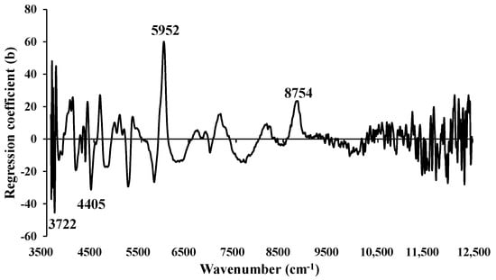
Figure 14.
Regression coefficient for the % of FC in chip biomass using the Full-PLSR method with a spectral preprocessing of constant offset.
Figure 14.
Regression coefficient for the % of FC in chip biomass using the Full-PLSR method with a spectral preprocessing of constant offset.

The Full-PLSR model with spectral preprocessing using the D1 provides improved model performance for % of FC in the ground biomass (Table 4). These results indicate that the reduction in linear shift and enhancement of the peaks in the raw spectra, achieved by applying the D1 with a gap and segment of 5, each contribute to the improvement in model accuracy.
3.3.4. Ash Content (%)
Table 2 presents the count of outliers for ash content in chip and ground biomass, based on reference and spectroscopic data. These identified outliers were removed from the total dataset, and various PLSR-based models were developed as explained in Section 2.6. For chip biomass, the best-performing model was developed using the MP PLSR 3-range methods with multi-preprocessing combination set of 5, 4, and 4. For ground biomass, the Full-PLSR model with spectral preprocessing from D1 provided the best performance results.
Figure 9d shows a scatter plot comparing the measured and predicted % ash content of non-wood and wood samples within the calibration and validation datasets. These results were obtained using the MP PLSR 3-range method. The most favorable outcomes were achieved through a spectral preprocessing combination set, consisting of the D2 from 3594.87 to 5492.59 cm−1, the D1 from 7498.31 to 5500.30 cm−1, and the D1 from 7506.02 to 12,489.48 cm−1, respectively (Table 3). The MP PLSR 3-range method enhances the explained variance by 4.6077%, while the Full-PLSR has an R2P of 0.7596.
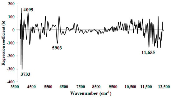
Figure 15.
Regression coefficient for the % of FC in ground biomass using Full-PLSR method with a spectral preprocessing of first derivative.
Figure 15.
Regression coefficient for the % of FC in ground biomass using Full-PLSR method with a spectral preprocessing of first derivative.
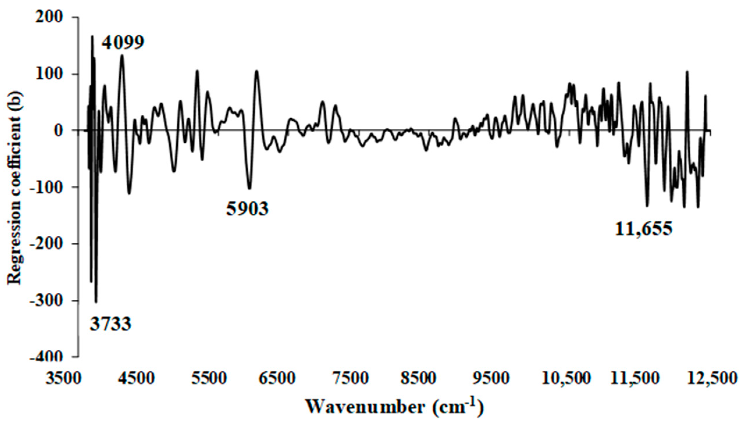
Figure 16 depicts the regression coefficient plot for the % ash content in chip biomass using the multi-preprocessing PLSR 3-range method, incorporating a combination set of 5, 4, and 4. The plot reveals significant peaks at 4019, 5285, 11,655, and 12,048 cm−1 (Table 5). These peaks are expected to have a substantial impact on achieving the highest-performing model for assessing the % ash content in chip biomass.
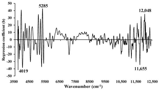
Figure 16.
Regression coefficient for the % of ash content in chip biomass using the MP PLSR 3-range method with a spectral multi-preprocessing combination set of 5, 4, and 4.
Figure 16.
Regression coefficient for the % of ash content in chip biomass using the MP PLSR 3-range method with a spectral multi-preprocessing combination set of 5, 4, and 4.

The best performance for % ash content in the ground biomass was achieved by using Full-PLSR with spectral preprocessing involving the D1, along with 13 LVs (Table 4). The results also indicate that removing baseline shift, resolving overlapping peaks, and highlighting the detailed structure in raw spectra will contribute to improving the model accuracy. In Figure 9h, a scatter plot illustrates the relationship between measured and predicted ash content percentages of non-wood and wood samples in both the calibration and validation sets, demonstrating the model high performance.
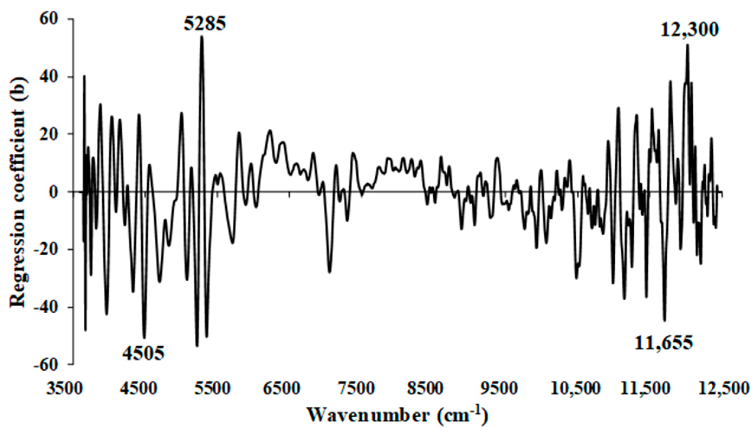
Figure 17 displays the regression coefficients for the % of ash content in the ground biomass using Full-PLSR with a spectral preprocessing technique involving the D1 (segment = 5 and gap = 5). The crucial peaks that may significantly impact the model performance are observed at wavenumbers 4505, 5285, 11,655, and 12,300 cm−1 (Table 5).
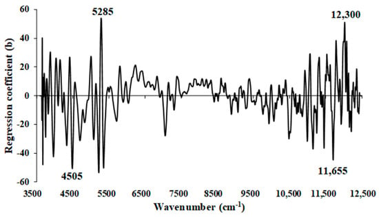
Figure 17.
Regression coefficient for the % of ash content in ground biomass using Full-PLSR method with a spectral preprocessing of D1.
Figure 17.
Regression coefficient for the % of ash content in ground biomass using Full-PLSR method with a spectral preprocessing of D1.
3.4. Limit of Quantification (LOQ)
In this study, the LOQ, defined as the lowest possible concentration of analyte that can be reliably detected and quantified with an acceptable level of accuracy and precision, is determined using the SD of the response and the slope obtained from the calibration set of the selected model [31]. Table 6 presents the LOQ results of the PLSR models for the percentages of MC, VM, FC, and ash content in both chip and ground biomass.
The LOQ for VM (%) in both chip and ground biomass, as well as for FC (%) in chip biomass, is below the minimum reference value used in the modeling. This suggests that the selected model for VM and FC in chip biomass has the potential to reliably detect and precisely quantify these parameters. This indicates its high sensitivity. For instance, the chosen MP method (PLSR 5-range) can reliably detect VM in both chip and ground biomass, as indicated by the model LOQ values, i.e., 23.4294% and 29.1656%, respectively. Similarly, using Full-PLSR with constant offset preprocessing, FC in chip biomass can be reliably detected with an LOQ value of 6.9125%.

Table 6.
LOQ results of PLSR models for the % of MC, VM, FC, and ash content in chip and ground biomass.
Table 6.
LOQ results of PLSR models for the % of MC, VM, FC, and ash content in chip and ground biomass.
| Parameter (%) | Category | Model | No. of Variables | Preprocessing | Reference Range | SD | Slope | LOQ (%) |
|---|---|---|---|---|---|---|---|---|
| MC | Chip | GA-PLSR | 57 | Second derivative | 12.21–2.21 | 0.71 | 1 | 7.06 |
| Ground | Full-PLSR | 1154 | Mean centering | 12.10–2.21 | 1.08 | 1 | 10.38 | |
| VM | Chip | MP-PLSR-5 range | 1150 | Combination set: 4, 4, 3, 2, 0 | 75.10–44.62 | 2.34 | 1 | 23.43 |
| Ground | MP-PLSR-5 range | 1150 | Combination set: 3, 5, 4, 5, 0 | 75.10–44.62 | 2.92 | 1 | 29.17 | |
| FC | Chip | Full-PLSR | 1154 | Constant offset | 42.05–10.40 | 2.09 | 1 | 6.91 |
| Ground | Full-PLSR | 1154 | First derivative | 42.05–13.23 | 1.90 | 1 | 19.04 | |
| Ash | Chip | MP-PLSR-3 range | 1154 | Combination set: 5, 4, 4 | 13.64–0.32 | 1.06 | 1 | 10.62 |
| Ground | Full-PLSR | 1154 | First derivative | 12.64–0.32 | 1.03 | 1 | 10.25 |
However, for other parameters, such as MC, ash, and FC in ground biomass, the LOQ values exceed the minimum reference value used in model development. This indicates that the selected models have limitations in assessing these parameters for not more than the minimum value of the model development. In Table 6, the slope of every model was the same but the SD of MC, ash, and FC was lower than VM, especially, for MC, the SD was very low leading to the high value of LOQ. Although the MC and FC were the constituents which were good absorbers of NIR radiation, in the case of LOQ calculation, this was not concerned with the absorption of radiation. However, the slope of the model and the SD of the data of the calibration set constituents must be high (wide range). Additionally, alternative modeling methods are considered for predicting proximate parameters, especially when their LOQ values surpass the minimum reference value used in modeling, which can enhance sensitivity as illustrated by the NIR model LOQ.
3.5. Effect of Combined Wood Samples with Non-Wood Samples in Developed Models
Table 7 presents the range of reference values for the % of MC, VM, FC, and ash content found in both wood and non-wood biomass samples within the calibration set and validation set. Based on Figure 9 and Table 7, the non-wood samples are characterized by a wider range in the MC, VM, FC, and ash content in both calibration and prediction sets. It becomes apparent that the range of each proximate parameter, whether in chip and ground form, widens after the inclusion of non-wood samples alongside the wood samples. This expansion aims to establish a more resilient PLSR model for predicting proximate parameters.
In Figure 9a,b, the range of MC (%) and VM (%) in wood chip biomass samples was narrower than that of non-wood samples, with the latter extending to both higher and lower percentages. Figure 9c illustrates that the range of FC values for wood samples was higher and narrower compared to that of the non-wood samples. The inclusion of non-wood samples expanded the range, mostly towards the lower percentage values. In contrast, Figure 9d, depicting ash content in chip biomass, reveals a lower and narrower range for both wood and non-wood samples compared to other proximate parameters. Consequently, the performance of the optimal model was comparatively lower for ash content in comparison to MC, VM, and FC.

Table 7.
The range of % of MC, VM, FC, and ash content of wood and non-wood samples in calibration and validation sets.
Table 7.
The range of % of MC, VM, FC, and ash content of wood and non-wood samples in calibration and validation sets.
| Biomass | Parameter (%) | Calibration Set | Validation Set | ||
|---|---|---|---|---|---|
| Wood | Non-Wood | Wood | Non-Wood | ||
| Chip | MC | 3.99–10.39 | 2.21–12.21 | 3.97–10.35 | 2.29–11.24 |
| VM | 48.31–69.74 | 44.62–75.10 | 49.63–67.29 | 44.84–70.59 | |
| FC | 18.95–42.05 | 10.4–39.55 | 20.67–38.55 | 13.23–35.46 | |
| Ash | 0.32–7.90 | 0.88–13.64 | 1.37–6.29 | 1.68–12.97 | |
| Ground | MC | 3.99–10.39 | 2.21–12.10 | 3.97–10.35 | 2.29–10.42 |
| VM | 48.31–69.74 | 44.62–75.10 | 49.63–67.29 | 44.84–70.59 | |
| FC | 13.23–42.05 | 15.69–41.48 | 20.67–38.55 | 15.33–35.46 | |
| Ash | 0.32–7.90 | 0.88–13.64 | 1.37–6.29 | 1.68–12.97 | |
Similarly, in ground biomass, the range of non-wood samples is higher compared to wood samples, except for FC. Similar to chip biomass, the range of MC (%) (Figure 9e) and VM (%) (Figure 9f) values for wood samples in ground biomass is narrower compared to that of the non-wood samples. Therefore, the inclusion of non-wood samples contributes to expanding the range to both higher and lower percentages. In Figure 9g, the percentage range of FC in wood samples is higher and wider compared to that of the non-wood samples. The inclusion of both wood and non-wood samples with a wider range has contributed to a better performance of the model compared to other parameters. From Figure 9h, the ash content (%) range in wood samples appears lower and narrower. However, the inclusion of non-wood samples towards higher % has notably expanded the ash content range, ultimately enhancing the model performance.
3.6. Comparison of the Model Performance between Chip and Ground Biomass
In this section, the performance of the best models for analyzing proximate parameters in chip and ground biomass was compared, as detailed in Table 3 and Table 4. The primary difference in the NIR scanning process was that chip biomass was scanned using the diffuse reflectance sphere macro sample rotating mode in a large amount, while ground biomass was scanned using the transflectance mode in a small amount. All other scanning conditions, including resolution, background scan time, sample scan time, and controlled laboratory settings, remained consistent, particularly in terms of temperature. The results revealed contrasting outcomes for chip and ground biomass, with chip biomass outperforming in all proximate parameters except for ash content. This observation is particularly significant when considering that ground biomass samples are typically more homogeneous. One possible explanation for this difference may be attributed to the scanning mode employed for biomass analysis, specifically the use of diffuse reflectance sphere macro sample rotating mode. Chip biomass samples inherently vary in particle size and shape, and introducing the sphere macro sample rotating mode during diffuse reflectance scanning allows the samples to rotate in a larger cup with more constituent variation, facilitating high-throughput screening and aiding in averaging any inhomogeneities, thereby providing a more representative measurement of the entire sample. Consequently, this enhanced scanning technique contributes to the improved performance observed in chip biomass analysis. During transflectance scanning, although light diffuses better within homogeneous materials, the sample size is very small and the constituent variation is minimal. Additionally, there may be a possibility of small NIR leakage via the glass vial edge, which might not provide useful information, resulting in comparatively lower performance compared to chip biomass analysis. For model of ash content, the chip model was poorer than the ground biomass model. The ash determination method by TGA in this experiment was by combustion up to 700 °C which is above 550 °C. Therefore, there is a risk in losing some of the potassium, and hence underestimating the ash content, while in chip, there was a full amount of these minerals.
3.7. Comparison with Previous Work
Several research studies have utilized NIR spectroscopy for proximate analysis of various biomass types. Typically, these studies have focused on specific biomass varieties. However, this study differs by developing models that encompass ten commonly used wood and non-wood biomass for energy purposes. The goal is to create a unified model for non-destructive assessment of proximate parameters. Unfortunately, the distribution of constituent parameters within both wood and non-wood is linear, resulting in a broad range for each parameter without clear separation into distinct groups. This study marks the first instance of combining these two types of data for estimation of proximate parameter analysis.
For MC analysis, Toscano et al. (2022) [21] conducted an evaluation of MC in industrial wood chips, analyzing a total of 817 samples. They reported R2P values ranging from 0.86 to 0.89. Similarly, Posom et al. (2022) [20] employed PLS regression to measure MC in cane bagasse, achieving an R2P value of 0.90. Sirisomboon et al. (2020) [22] assessed MC in bamboo chips, obtaining an R2P value of 0.96, while Adnan et al. (2017) [25] predicted the MC in intact green coffee beans, resulting in an R2P value of 0.96. Shrestha et al. (2018) [23] evaluated MC in bamboo chips using NIR-gun (600−1100 nm) and reported an R2P value of 0.92, whereas they achieved an R2P value of 0.74 using Micro-NIR (1150−215 nm). Similarly, Xue et al. (2015) [51] measured MC in corn stover with an R2C value of 0.81. In this study, the model performance is comparatively lower for both chip (R2P = 0.8654) and ground (R2P = 0.7868) biomass compared to the previous research mentioned above.
Similarly, for VM analysis for non-wood sample, previous research recorded R2P values of 0.81 for chip bamboo [22], 0.82 for ground bamboo [24], and 0.68 for corn stover [51]. In this study, the R2P for VM in chip biomass (0.79) and ground biomass (0.77) are both lower when compared to the chip bamboo [22] and ground bamboo [24], respectively. However, when compared to the performance of corn stover, both the chip and ground combined wood and non-wood models exhibited better performance.
For FC, previous research recorded R2P values of 0.81 for chip bamboo [22], 0.66 for corn stover [51], and 0.85 for ground bamboo [24]. The model performance for FC in this study on chip biomass (R2P = 0.88) is better compared to the previous study.
For ash, being inorganic, it does not absorb NIR radiation [22,24]. However, the model developed for ash content in wood and non-wood chip (R2P of 0.7946) and ground biomass of wood and non-wood (R2P of 0.8005) in this study proves to be a reliable predictor. Previous research of non-wood model has reported R2P values of 0.86 for chip bamboo [22], 0.85 for corn stover [51], and 0.51 for ground bamboo [24]. Compared to the previous study, the performance of chip combined wood and non-wood is lower compared to chip bamboo [22] and corn stover [51]. However, the performance of ground combined model is comparatively higher than that of ground bamboo [24].
As recommended by Williams et al. (2019) [45], a model achieving an R2 of 0.83−0.90 can be cautiously utilized for most applications, including research and from 0.66 to 0.81 is considered suitable for rough screening. Moreover, based on Zornoza et al. (2008) [46], an RPD value between 2 and 2.5 enables approximate quantitative predictions and 2.5 and 3 are indicative of good prediction. Therefore, the model selected in this research for non-destructive MC (R2P of 0.8654 and RPD of 2.9) and FC (R2P of 0.8773 and RPD of 3) assessment in chip biomass can be cautiously employed for most applications, including research while the other models, i.e., VM and ash models from chip and MC, VM, FC, and ash model from ground biomass can be applied for screening purposes only (R2P of 0.7733−0.8005 and RPD was 2.2−2.3). Therefore, it is advisable to employ the chosen model derived from chip wood and non-wood when evaluating proximate parameters for practical applications, particularly MC and FC.
4. Conclusions
In this study, proximate parameters (MC, VM, FC, and ash content) were determined using a TGA. PLSR models were developed and compared utilizing NIR spectroscopy within a wavenumber range from 3594.87 to 12,489.48 cm−1 to assess these proximate analysis parameters, both in chip and ground biomass. These models were constructed from raw spectra, traditional preprocessing approaches, GA, SPA, and spectral MP with 5-range and 3-range methods.
The findings of this study underscore the potential of NIR spectroscopy as a promising alternative tool for the quantitative prediction of MC and FC in chip biomass. The selected model for MC and FC in chip biomass is suitable for most applications, including research, but should be used with caution. As for the remaining proximate parameters, i.e., MC and FC in ground biomass, and VM and ash content in both chip and ground biomass, the models exhibit fair performance and are primarily suitable for rough screening purposes. The models perform more accurately in chip biomass, highlighting the efficacy of diffuse reflectance sphere macro sample rotating mode compared to the transflectance mode of scanning in ground biomass. In addition, the chip biomass model can be preferred for proximate analysis instead of the ground biomass model, as it eliminates the need for biomass grounding, saving time, labor, and costs prior to scanning.
The model developed in this study proved to be more robust than those in previous studies. This is attributed to the wider variation in different types of biomass, including fast-growing trees and agricultural residues, whereas previous studies were focused on specific biomass species. The accuracy, robustness, and sensitivity of these models can be further enhanced by expanding the dataset with samples from diverse sources and validating their performance with unknown samples before industrial application. Implementing the selected models will benefit researchers, engineers, and industries aiming to design thermochemical conversion systems that can select a suitable biomass and efficiently extract maximum energy, all while minimizing energy consumption, optimized process, and environmental impact.
Author Contributions
Conceptualization, B.S., J.P., P.S., P.P. and B.P.S.; methodology, B.S., J.P., P.S. and B.P.S.; software, B.S. and J.P.; formal analysis, B.S. and J.P.; investigation, B.S.; resources, B.S. and B.P.S.; data curation, B.S., J.P. and P.S.; writing—original draft, B.S.; writing—review and editing, B.S., J.P., P.S., B.P.S., P.P. and A.F.; visualization, B.S.; supervision, J.P., P.S., B.P.S., P.P. and A.F.; project administration, P.S.; funding acquisition, P.S.; validation, B.P.S. and A.F. All authors have read and agreed to the published version of the manuscript.
Funding
This research received funding from the King Mongkut’s Institute of Technology Ladkrabang (KMITL), Thailand, through the KMITL doctoral scholarship KDS 2020/52). Additionally, the APC was partially funded by the School of Engineering, KMITL, Bangkok, Thailand.
Data Availability Statement
Data is contained within the article.
Acknowledgments
The authors would like to express their sincere gratitude to the Near-Infrared Spectroscopy Research Center for Agricultural Product and Food (www.nirsresearch.com), Department of Agricultural Engineering, School of Engineering at King Mongkut’s Institute of Technology Ladkrabang, Bangkok, Thailand, for their generous research funding support provided through the KMITL doctoral scholarship (KDS 2020/052).
Conflicts of Interest
The authors declare no conflicts of interest.
Abbreviations
| D1 | first derivative |
| D2 | second derivative |
| DTG | derivative thermogravimetric |
| FC | fixed carbon |
| FT | Fourier transform |
| g | gap |
| GA | genetic algorithm |
| LVs | number of latent variables |
| LOQ | limit of quantification |
| Max | maximum |
| MC | moisture content |
| Min | minimum |
| Mean | average |
| MSC | multiplicative scatter correction |
| MP | multi-preprocessing |
| N | nitrogen |
| NT | total number of sample |
| Nc | number of sample in calibration set |
| Np | number of sample in prediction set |
| NIRS | near-infrared spectroscopy |
| O | oxygen |
| PLSR | partial least squares regression |
| R2 | coefficient of determination |
| R2C | coefficient of determination of calibration set |
| R2P | coefficient of determination of prediction set |
| RPD | ratio of prediction to deviation |
| RMSE | root mean square error |
| s | segment |
| SC | slope of the regression line |
| SD | standard deviation |
| SEC | standard error of calibration set |
| SEL | standard error of laboratory |
| SEP | standard error of prediction set |
| SNV | standard normal variate |
| SPA | successive projection algorithm |
| SW | selected wavenumber |
| TG | thermogravimetric |
| VM | volatile matter |
| σC | standard deviation of residual of calibration set |
References
- Zhang, Y.; Wang, H.; Sun, X.; Wang, Y.; Liu, Z. Separation and Characterization of Biomass Components (Cellulose, Hemicellulose, and Lignin) from Corn Stalk. BioResources 2021, 16, 7205–7219. [Google Scholar] [CrossRef]
- Nimmanterdwong, P.; Chalermsinsuwan, B.; Piumsomboon, P. Prediction of lignocellulosic biomass structural components from ultimate/proximate analysis. Energy 2021, 222, 119945. [Google Scholar] [CrossRef]
- Saldarriaga, J.F.; Aguado, R.; Pablos, A.; Amutio, M.; Olazar, M.; Bilbao, J. Fast characterization of biomass fuels by thermogravimetric analysis (TGA). Fuel 2015, 140, 744–751. [Google Scholar] [CrossRef]
- Teh, J.S.; Teoh, Y.H.; How, H.G.; Sher, F. Thermal Analysis Technologies for Biomass Feedstocks: A State-of-the-Art Review. Processes 2021, 9, 1610. [Google Scholar] [CrossRef]
- Demirbas, A. Combustion characteristics of different biomass fuels. Prog. Energy Combust. Sci. 2004, 30, 219–230. [Google Scholar] [CrossRef]
- Aich, S.; Behera, D.; Nandi, B.K.; Bhattacharya, S. Relationship between proximate analysis parameters and combustion behaviour of high ash Indian coal. Int. J. Coal Sci. 2020, 7, 766–777. [Google Scholar] [CrossRef]
- Demirbas, A. Effects of moisture and hydrogen content on the heating value of fuels. Energy Source Part A 2007, 29, 649–655. [Google Scholar] [CrossRef]
- García, R.; Pizarro, C.; Lavín, A.G.; Bueno, J.L. Biomass proximate analysis using thermogravimetry. Bioresour. Technol. 2013, 139, 1–4. [Google Scholar] [CrossRef] [PubMed]
- Kongto, P.; Palamanit, A.; Ninduangdee, P.; Singh, Y.; Chanakaewsomboon, I.; Hayat, A.; Wae-hayee, M. Intensive exploration of the fuel characteristics of biomass and biochar from oil palm trunk and oil palm fronds for supporting increasing demand of solid biofuels in Thailand. Energy Rep. 2022, 8, 5640–5652. [Google Scholar] [CrossRef]
- Jia, Y.; Li, Z.; Wang, Y.; Wang, X.; Lou, C.; Xiao, B.; Lim, M. Visualization of Combustion Phases of Biomass Particles: Effects of Fuel Properties. ACS Omega 2021, 6, 27702–27710. [Google Scholar] [CrossRef]
- Vassilev, S.V.; Vassileva, C.G.; Song, Y.-C.; Li, W.-Y.; Feng, J. Ash contents and ash-forming elements of biomass and their significance for solid biofuel combustion. Fuel 2017, 208, 377–409. [Google Scholar] [CrossRef]
- Pazó, J.A.; Granada, E.; Saavedra, A.; Eguía, P.; Collazo, J. Biomass thermogravimetric analysis: Uncertainty determination methodology and sampling maps generation. Int. J. Mol. Sci. 2010, 11, 2701–2714. [Google Scholar] [CrossRef]
- Özyuğuran, A.; Yaman, S. Prediction of calorific value of biomass from proximate analysis. Energy Procedia 2017, 107, 130–136. [Google Scholar] [CrossRef]
- ASTM E871-82(2019); Standard Test Method for Moisture Analysis of Particulate Wood Fuels. ASTM: West Conshohocken, PA, USA, 2019.
- ASTM E872-82(2019); Standard Test Method for Volatile Matter in the Analysis of Particulate Wood Fuels. ASTM: West Conshohocken, PA, USA, 2019.
- ASTM E1755-01(2020); Standard Test Method for Ash in Biomass. ASTM: West Conshohocken, PA, USA, 2020.
- Sahito, A.R.; Mahar, R.; Siddiqui, Z.; Brohi, K. Estimating calorific values of lignocellulosic biomass from volatile and fixed solids. Int. J. Renew. Energy Res. 2013, 2, 1–6. [Google Scholar]
- Posom, J.; Maraphum, K.; Phuphaphud, A. Rapid Evaluation of Biomass Properties Used for Energy Purposes Using Near-Infrared Spectroscopy. In Renewable Energy-Technologies and Applications; IntechOpen: London, UK, 2020. [Google Scholar]
- Torquato, L.D.M.; Crnkovic, P.M.; Ribeiro, C.A.; Crespi, M.S. New approach for proximate analysis by thermogravimetry using CO2 atmosphere: Validation and application to different biomasses. J. Therm. Anal. Calorim. 2017, 128, 1–14. [Google Scholar] [CrossRef]
- Posom, J.; Phuphaphud, A.; Saengprachatanarug, K.; Maraphum, K.; Saijan, S.; Pongkan, K.; Srimai, K. Real-time measuring energy characteristics of cane bagasse using NIR spectroscopy. Sens. Bio-Sens. Res. 2022, 38, 100519. [Google Scholar]
- Toscano, G.; Leoni, E.; Gasperini, T.; Picchi, G. Performance of a portable NIR spectrometer for the determination of moisture content of industrial wood chips fuel. Fuel 2022, 320, 123948. [Google Scholar] [CrossRef]
- Sirisomboon, P.; Funke, A.; Posom, J. Improvement of proximate data and calorific value assessment of bamboo through near infrared wood chips acquisition. Renew. Energy 2020, 147, 1921–1931. [Google Scholar] [CrossRef]
- Shrestha, A.; Sirisomboon, P. Rapid evaluation of moisture content in bamboo chips using diode array near infrared spectroscopy. MATEC Web Conf. —ICEAST 2018 2018, 192, 03020. [Google Scholar] [CrossRef][Green Version]
- Posom, J.; Sirisomboon, P. Evaluation of the higher heating value, volatile matter, fixed carbon and ash content of ground bamboo using near infrared spectroscopy. J. Near Infrared Spectrosc. 2017, 25, 301–310. [Google Scholar] [CrossRef]
- Adnan, A.; Hörsten, D.V.; Pawelzik, E.; Mörlein, A.D. Rapid Prediction of Moisture Content in Intact Green Coffee Beans Using Near Infrared Spectroscopy. Foods 2017, 6, 38. [Google Scholar] [CrossRef]
- Shrestha, B.; Posom, J.; Sirisomboon, P.; Shrestha, B.P. Comprehensive Assessment of Biomass Properties for Energy Usage Using Near-Infrared Spectroscopy and Spectral Multi-Preprocessing Techniques. Energies 2023, 16, 5351. [Google Scholar] [CrossRef]
- Li, M.; He, S.; Wang, J.; Liu, Z.; Xie, G.H. An NIRS-based assay of chemical composition and biomass digestibility for rapid selection of Jerusalem artichoke clones. Biotechnol. Biofuels 2018, 11, 334. [Google Scholar] [CrossRef]
- Assis, C.; Ramos, R.S.; Silva, L.A.; Kist, V.; Barbosa, M.H.P.; Teofilo, R.F. Prediction of Lignin Content in Different Parts of Sugarcane Using Near-Infrared Spectroscopy (NIR), Ordered Predictors Selection (OPS), and Partial Least Squares (PLS). Appl. Spectrosc. 2017, 71, 2001–2012. [Google Scholar] [CrossRef]
- Li, Z.; Song, J.; Ma, Y.; Yu, Y.; He, X.; Guo, Y.; Dou, J.; Dong, H. Identification of aged-rice adulteration based on near-infrared spectroscopy combined with partial least squares regression and characteristic wavelength variables. Food Chem. X 2023, 17, 100539. [Google Scholar] [CrossRef] [PubMed]
- Singh, S.B.; De, M. Alumina based doped templated carbons: A comparative study with zeolite and silica gel templates. Microporous Mesoporous Mater. 2018, 257, 241–252. [Google Scholar] [CrossRef]
- Stolov, A.A.; Simoff, D.A.; Li, J. Thermal stability of specialty optical fibers. J. Light. Technol. 2008, 26, 3443–3451. [Google Scholar] [CrossRef]
- Díez, D.; Urueña, A.; Piñero, R.; Barrio, A.; Tamminen, T. Determination of Hemicellulose, Cellulose, and Lignin Content in Different Types of Biomasses by Thermogravimetric Analysis and Pseudocomponent Kinetic Model (TGA-PKM Method). Processes 2020, 8, 1048. [Google Scholar] [CrossRef]
- López-González, D.; Fernandez-Lopez, M.; Valverde, J.L.; Sanchez-Silva, L. Thermogravimetric-mass spectrometric analysis on combustion of lignocellulosic biomass. Bioresour. Technol. 2013, 143, 562–574. [Google Scholar] [CrossRef] [PubMed]
- Shrestha, B.; Shrestha, Z.; Posom, J.; Sirisomboon, P.; Shrestha, B.P. Evaluating limit of detection and quantification for higher heating value and ultimate analysis of fast-growing trees and agricultural residues biomass using NIRS. EASR 2023, 50, 612–618. [Google Scholar]
- Broad, N.; Graham, P.; Hailey, P.; Hardy, A. Guidelines for the development and validation of near-infrared spectroscopic methods in the pharmaceutical industry. Handb. Vib. Spectrosc. 2002, 5, 3590–3610. [Google Scholar]
- Roger, J.-M.; Mallet, A.; Marini, F. Preprocessing NIR Spectra for Aquaphotomics. Molecules 2022, 27, 6795. [Google Scholar] [CrossRef] [PubMed]
- Robert, G.; Gosselin, R. Evaluating the impact of NIR pre-processing methods via multiblock partial least-squares. Anal. Chim. Acta 2022, 1189, 339255. [Google Scholar] [CrossRef]
- Jiang, W.; Lu, C.; Zhang, Y.; Ju, W.; Wang, J.; Hong, F.; Wang, T.; Ou, C. Moving-window-improved Monte Carlo uninformative variable elimination combining successive projections algorithm for near-infrared spectroscopy (NIRS). J. Spectrosc. 2022, 2020, 3590301. [Google Scholar] [CrossRef]
- Koljonen, J.; Nordling, T.E.; Alander, J.T. A review of genetic algorithms in near infrared spectroscopy and chemometrics: Past and future. J. Near Infrared Spectrosc. 2008, 16, 189–197. [Google Scholar] [CrossRef]
- Fei, Q.; Li, M.; Wang, B.; Huan, Y.; Feng, G.; Ren, Y. Analysis of cefalexin with NIR spectrometry coupled to artificial neural networks with modified genetic algorithm for wavelength selection. Chemometr. Intell. Lab. Syst. 2009, 97, 127–131. [Google Scholar] [CrossRef]
- Maraphum, K.; Ounkaew, A.; Kasemsiri, P.; Hiziroglu, S.; Posom, J. Wavelengths Selection Based on Genetic Algorithm (GA) and Successive Projections Algorithms (SPA) Combine With PLS Regression for Determination the Soluble Solids Content in Nam-DokMai Mangoes Based on Near Infrared Spectroscopy. Eng. Appl. Sci. Res. 2021, 49, 119–126. [Google Scholar]
- Araújo, M.C.U.; Saldanha, T.C.B.; Galvão, R.K.H.; Yoneyama, T.; Chame, H.C.; Visani, V. The successive projections algorithm for variable selection in spectroscopic multicomponent analysis. Chemometr. Intell. Lab. Syst. 2001, 57, 65–73. [Google Scholar] [CrossRef]
- Chen, Y.M.; Lin, P.; He, Y.; He, J.Q.; Zhang, J.; Li, X.L. Fast quantifying collision strength index of ethylene-vinyl acetate co-polymer coverings on the fields based on near infrared hyperspectral imaging techniques. Sci. Rep. 2016, 6, 20843. [Google Scholar] [CrossRef]
- Li, C.; He, M.; Cai, Z.; Qi, H.; Zhang, J.; Zhang, C. Hyperspectral Imaging with Machine Learning Approaches for Assessing Soluble Solids Content of Tribute Citru. Foods 2023, 12, 247. [Google Scholar] [CrossRef]
- Williams, P.; Manley, M.; Antoniszyn, J. Near Infrared Technology: Getting the Best out of Light; African Sun Media: Stellenbosch, South Africa, 2019. [Google Scholar]
- Zornoza, R.; Guerrero, C.; Mataix-Solera, J.; Scow, K.M.; Arcenegui, V.; Mataix-Beneyto, J. Near infrared spectroscopy for determination of various physical, chemical and biochemical properties in Mediterranean soils. Soil Biol. Biochem. 2008, 40, 1923–1930. [Google Scholar] [CrossRef] [PubMed]
- Guideline, I.H.T. Validation of analytical procedures: Text and methodology. Q2 (R1) 2005, 1, 5. [Google Scholar]
- Werther, J.; Saenger, M.; Hartge, E.-U.; Ogada, T.; Siagi, Z. Combustion of agricultural residues. Prog. Energy Combust. Sci. 2000, 26, 1–27. [Google Scholar] [CrossRef]
- Yuan, Y.; Yong, H.; Tan, J.; Wang, Y.; Kumar, S.; Wang, Z. Co−Combustion characteristics of typical biomass and coal blends by thermogravimetric analysis. Front. Energy Res. 2021, 9, 753622. [Google Scholar] [CrossRef]
- Workman, J., Jr.; Weyer, L. Practical Guide to Interpretive Near-Infrared Spectroscopy; CRC Press: Boca Raton, FL, USA, 2007. [Google Scholar]
- Xue, J.; Yang, Z.; Han, L.; Liu, Y.; Liu, Y.; Zhou, C. On-line measurement of proximates and lignocellulose components of corn stover using NIRS. Appl. Energy 2015, 137, 18–25. [Google Scholar] [CrossRef]
Disclaimer/Publisher’s Note: The statements, opinions and data contained in all publications are solely those of the individual author(s) and contributor(s) and not of MDPI and/or the editor(s). MDPI and/or the editor(s) disclaim responsibility for any injury to people or property resulting from any ideas, methods, instructions or products referred to in the content. |
© 2024 by the authors. Licensee MDPI, Basel, Switzerland. This article is an open access article distributed under the terms and conditions of the Creative Commons Attribution (CC BY) license (https://creativecommons.org/licenses/by/4.0/).

