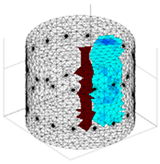
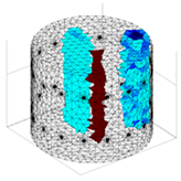
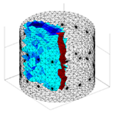
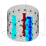
Abstract
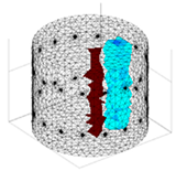
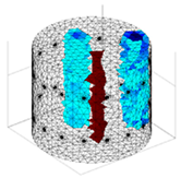
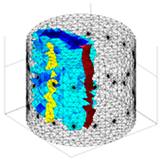
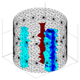
This paper presents innovative machine-learning solutions to enhance energy efficiency in electrical tomography for industrial reactors. Addressing the key challenge of optimizing the neural model’s loss function, a classifier tailored to precisely recommend optimal loss functions based on the measurement data is designed. This classifier recommends which model, equipped with given loss functions, should be used to ensure the best reconstruction quality. The novelty of this study lies in the optimal adjustment of the loss function to a specific measurement vector, which allows for better reconstructions than that by traditional models trained based on a constant loss function. This study presents a methodology enabling the development of an optimal loss function classifier to determine the optimal model and loss function for specific datasets. The approach eliminates the randomness inherent in traditional methods, leading to more accurate and reliable reconstructions. In order to achieve the set goal, four models based on a simple LSTM network structure were first trained, each connected with various loss functions: HMSE (half mean squared error), Huber, l1loss (L1 loss for regression tasks—mean absolute error), and l2loss (L2 loss for regression tasks—mean squared error). The best classifier training results were obtained for support vector machines. The quality of the obtained reconstructions was evaluated using three image quality indicators: PSNR, ICC, and MSE. When applied to simulated cases and real measurements from the Netrix S.A. laboratory, the classifier demonstrated effective performance, consistently recommending models that produced reconstructions that closely resembled the real objects. Such a classifier can significantly optimize the use of EIT in industrial reactors by increasing the accuracy and efficiency of imaging, resulting in improved energy management and efficiency.
1. Introduction
Modern industrial reactors are currently struggling with the need to increase energy efficiency. While rooted in environmental considerations, this imperative is equally driven by economic demands, particularly the need to reduce operating costs. Achieving such a goal requires the design of advanced reactors and precise monitoring of internal processes. The use of advanced imaging methods using tomographic technologies facilitates observation, offers detailed understanding, and enables the real-time optimization of reactor processes. The result is measurable improvements in energy savings and operational efficiency.
Beyond energy efficiency, industrial reactors are an integral part of several industries. In the chemical industry, they are critical for producing essential chemicals, intermediates, and polymers. The petrochemical industry uses them to refine crude oil into products such as fuels and plastics. In the food industry, reactors facilitate processes such as fermentation and pasteurization, ensuring food safety and nutrition [1,2,3,4]. The pharmaceutical industry also relies on reactors, particularly for drug synthesis, and is adopting continuous flow processes in milli- or microreactors that efficiently handle extreme reactions and are revolutionizing the industry.
In this context, the rigorous monitoring of industrial reactors becomes paramount. The objective is two-fold: ensuring operational efficacy and emphasizing energy efficiency. Over the last century, the way industrial processes are monitored has undergone a significant transformation. Initially, the focus was on detecting anomalies, but over time they have expanded their scope to include diagnosing root causes and even predicting impending problems. This evolution, as pointed out by Reis and Gins, reflects the increasing complexity and sophistication of monitoring techniques that have become indispensable to modern industrial operations [5]. Anomaly detection, as a core technology, has played a key role in ensuring the safety and reliability of the system [6]. In recent years, preventive maintenance, especially for machinery, has become increasingly important as a strategic approach to optimizing operations and ensuring longevity [7]. Industries can increase operational efficiency by anticipating and resolving potential problems before they escalate.
However, monitoring these complex industrial processes, especially those in tank reactors, presents unique challenges. Tank reactors experience a variety of physical and chemical reactions, can involve phase changes, and are used in processes based on chemical reactions. Such processes are dynamic and can have non-uniform distributions, making modelling difficult. The design of the reactor, including factors such as its diameter, shape, capacity, and wall material, also affects the course of the process. Some reactors, known as heterogeneous reactors, simultaneously handle multiple states of matter, adding another layer of complexity to their monitoring and efficiency optimization [8].
Given the critical nature of industrial reactors, their careful maintenance and monitoring should ensure operational safety in terms of performance and operational reliability. Any oversight in their maintenance can have serious consequences regarding human safety and economic impact. Ensuring their optimal and safe operation is about maintaining product quality and protecting the environment and employees [9].
In the past, reactor maintenance was mostly scheduled, resulting in unnecessary downtime or unexpected malfunctions. However, the integration of artificial intelligence (AI) and the Internet of Things (IoT) with the advent of Industry 4.0 has changed this paradigm [10]. Predictive maintenance, using AI techniques such as machine learning and deep learning, is now at the forefront. Recent research has highlighted the surge in publications focused on AI techniques tailored for predictive maintenance, with emergent paradigms such as machine learning and deep learning making notable contributions [11]. The emphasis now is on predictive maintenance, underpinned by real-time data and advanced algorithms, all converging towards the ultimate objective of enhanced energy efficiency. Innovations such as wireless sensors for monitoring equipment in research reactors highlight the potential of these modern maintenance techniques [12]. Such systems enable real-time monitoring and analysis, aiding in decisions centered on energy optimization.
Direct observation of the reactor interior often proves to be extremely challenging and relies on the analysis of fundamental physical parameters such as temperature, pressure, and flow rate for evaluation. While these metrics provide valuable insight, they are inherently point measurements that provide only a limited approximation of the complex internal state of the reactor [13]. In the past, monitoring methods have mainly used intrusive sensors, which, while useful, carry the risk of disrupting the delicate process conditions within the reactor.
With the evolution of the industrial landscape, there was a noticeable shift away from traditional maintenance strategies largely based on scheduled inspections. The current focus is on predictive maintenance, a sophisticated approach that leverages real-time sensor data combined with advanced algorithms. This paradigm anticipates potential component failures and orchestrates timely interventions to ensure seamless reactor operation, all while championing increased energy efficiency [10].
In this context, techniques such as electrical tomography have emerged as game-changers. Unlike their invasive counterparts, these non-invasive monitoring tools offer a more comprehensive perspective. In particular, electrical tomography is distinguished by its ability to image objects comprehensively, providing a holistic view of the object’s internal dynamics [14,15]. Two prominent non-invasive imaging techniques have emerged as leaders in this field: electrical capacitance tomography (ECT) [16,17,18,19,20,21,22,23,24] and electrical impedance tomography (EIT) [25,26,27,28,29,30,31,32,33]. Unlike ECT, EIT captures impedance characteristics and dielectric properties, providing a richer dataset and thus a more detailed insight into the ongoing processes inside the reactor [31]. In addition, EIT’s adaptability to complex scenarios, such as those involving multiple bubbles, and its ability to provide enhanced accuracy in image reconstruction position it as a superior choice for comprehensive reactor monitoring. Its robustness to noise and its ability to accurately determine the size and shape of bubbles, especially in a dynamically changing environment, make EIT a more reliable tool for industrial applications [31].
Electrical tomography is often used to monitor and track dynamic processes in the industry. EIT can also be used to visualize moisture distribution inside walls, a critical issue in building maintenance due to the detrimental effects of moisture, such as accelerated wear of facades and paint coatings and weakening of wall structures [34]. Research on industrial reactors was also carried out. Zhu et al. present an algorithm that increases the accuracy of image reconstruction in EIT technology, especially in complicated cases with many bubbles, based on the example of such a reactor model [31]. Following this, Kłosowski et al. introduced a novel concept for monitoring industrial tank reactors using a hybrid method of electrical capacitance and impedance tomography [15].
However, the journey of electrical tomography is not without its challenges. One of the primary obstacles is the ill-posed inverse problem, which poses difficulties in acquiring high-resolution tomographic images. When compounded with noisy input data, this challenge becomes even more daunting. Recent research has introduced innovative machine learning methodologies for intelligent selection based on the reconstruction case [16] to address this. Another study has explored the economic and production implications of curtailing industrial energy consumption [35]. This research underscores the critical role of top-tier management in energy conservation and accentuates the significance of maintenance planning and control in ensuring consistently reduced energy consumption.
The use of machine learning methods, particularly neural networks, to address the challenge of inverse tomography represents a notable advance in industrial reactor monitoring. By skillfully managing complex and multidimensional datasets, these approaches improve reactor interior’s visualization accuracy and effectiveness, improving process monitoring and reliability [15]. The implementation of large datasets in machine learning has revolutionized the field, allowing for more nuanced and sophisticated model training. These extensive datasets provide a rich source of information, enhancing the model’s ability to generalize and perform accurately in diverse and complex scenarios [36,37]. At the heart of deep learning, a subset of machine learning, is the intricate process of optimization that ensures a model can make accurate predictions based on the data on which it is trained. This training process’s effectiveness is paramount, especially given the computational demands and long timescales often required for model convergence. Such computational challenges have increased reliance on advanced graphics processing units (GPUs) to speed up training [38]. Central to the optimization process is the loss function. This mathematical construct is primarily derived from the training dataset and serves as the guiding objective for the optimization procedure. The loss function quantifies the difference or discrepancy between the model’s predictions and the actual ground truth values. It measures the performance of the model and indicates areas where improvements are needed [39].
In the research presented here, several loss functions have been proposed and used for regression tasks where the goal is to predict a continuous value. Among them, mean absolute error (MAE) and mean squared error (MSE) are perhaps the most widely used [40,41,42]. MSE, with its quadratic nature, is particularly suitable for gradient descent optimization due to its smooth derivability [40]. However, its sensitivity to outliers can sometimes be a drawback, potentially leading to models that are overly influenced by anomalous data points. On the other hand, MAE, being linear, is inherently more robust to outliers. However, its computational requirements, especially for derivatives, can be a limitation [41]. Recognizing the strengths and weaknesses of both MSE and MAE, researchers have proposed hybrid approaches. One notable example is the Huber loss function, which attempts to combine the best of both worlds. The Huber function reduces sensitivity to outliers, similar to MAE, while retaining the desirable derivability properties of MSE, making it particularly suitable for gradient-based optimization methods [43].
The primary objective of this study is to increase the maintenance energy efficiency and reliability of industrial reactors by optimizing the loss function for neural network models used in electrical tomography. Traditionally, the selection of an appropriate loss function for such models has often been based on trial and error or the intuition and experience of the researcher. While sometimes effective, this approach lacks systematicity and can lead to suboptimal results, especially when dealing with complex datasets and complicated image reconstruction tasks.
A specially adapted classifier has been designed to optimize the loss function based on measurement data to solve this problem. This classifier acts as a guide, indicating which model, associated with various loss functions, should be used to ensure the highest image reconstruction quality. This systematic approach eliminates the randomness and guesswork traditionally associated with model and loss function selection. It ensures that the chosen model is best suited to the specific dataset, resulting in more accurate and reliable reconstructions. To achieve this goal, we first trained four models based on a simple LSTM network structure, each paired with different loss functions: HMSE (half mean squared error), Huber, l1loss (L1 loss for regression tasks—mean absolute error), and l2loss (L2 loss for regression tasks—mean squared error). It is important to note that the primary focus of this study was not to innovate a new, more efficient neural network structure. Therefore, a simple LSTM network was considered appropriate for our experiments.
The novelty of our approach lies in the creation of a classifier that can determine the most optimal model and loss function; through this, we are paving the way for more consistent and higher quality image reconstructions in electrical tomography.
This paper is divided into four main chapters. After the introduction, the Section 2 details the experimental setup, which consists of an industrial tank reactor model equipped with EIT electrodes and a prototype hybrid tomograph. In this section, the network architecture is explored, various loss functions are examined, and a classifier’s training and testing processes designed to recommend the most appropriate model based on measurement data are described. In the Results and Discussion section, the reconstructions obtained from different models using different loss functions and the results of the classifier operation are presented, using both simulation data and real measurements of the reactor. In addition, quantitative metrics used to assess image quality are presented. The final chapter provides a concise summary of the research results.
2. Materials and Methods
This section contains the methodology and technical intricacies of using electrical impedance tomography (EIT) to image the internal structures of industrial reactors. The focus of the research was an industrial model of a tank reactor equipped with EIT electrodes and a prototype of a hybrid tomograph. The inverse and forward problems with EIT are discussed. The network architecture is presented, emphasizing the importance of selecting the appropriate loss function for neural network models. After an in-depth examination of various loss functions, this chapter discusses the training and testing processes of a classifier designed to recommend an optimal model based on measurement data.
2.1. Hardware
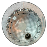
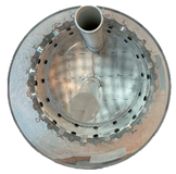
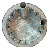
A hybrid tomography system (Figure 1) was developed and established in the Netrix S.A laboratory and used for this investigation. The main component of this apparatus is the STM32F103VCT6 microcontroller (STMicroelectronics, Geneva, Switzerland), which orchestrates the measurement routines and electrode setup specifications. The instrument has a modular electrode system, making it versatile for electrical impedance tomography (EIT) and electrical capacitance tomography (ECFT) methods. This dual capability increases the adaptability of the instrument. However, the tool was used strictly in this investigation’s EIT methodology.
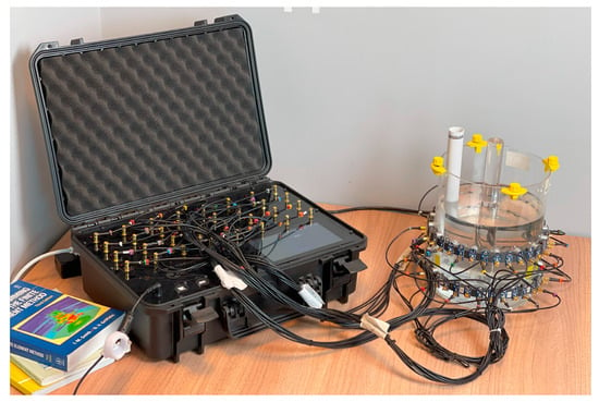
Figure 1.
Electrical impedance tomography connected to the reactor model.
Within the architectural blueprint of the analyzed tomographic device, a sophisticated nexus formed by Intel Altera Cyclone IV and Cyclone V FPGA silicon arrays emerges. The designed solution facilitates the deployment of concurrent functional modules, each exhibiting autonomy per channel. Central to this intricate apparatus is the primary circuit board, a hub of energy dissemination and excitation current modulation. This board provides an intricate lattice for data address bus connectivity amongst the isolated segments and possesses a transformative power modulator. This converter adeptly morphs the 12 V DC input (harnessed from an embedded battery) into the necessary voltage tiers vital for the optimal operation of various functional units. Integrated into this power module is a battery management and regeneration system. The main board generates excitation currents, embedded in an internal system that ensures signal integrity and confirms accurate electrode alignment. Another pivotal component is the diagnostic measurement unit, fortified with four dynamic electrodes. These electrodes house sophisticated mechanisms tailored for signal modulation, precise gain calibration, and critical zero-intersection detection. This latter function, aligned with the X-axis, is instrumental in deciphering wave amplitude and associated phase deviations. In a harmonious confluence with the Cyclone IV FPGA architecture and the precision of the ADS8588 A/D transducer(Analog Devices, Norwood, MA, USA), an analytical ensemble emerges. This ensemble orchestrates meticulous tasks ranging from signal refinement to RMS computation and phase signal monitoring.
The embryonic data embark on a journey via interlinked buses to the command hub, a marvel that integrates eight distinct Cyclone IV frameworks. Embedded in the data storage modulus is a powerful ARM Cortex-A9 dual-core CPU that interfaces seamlessly with FPGAs (Field Programmable Gate Arrays) located in the Intel Altera Cyclone V domain. This component is entrusted with disseminating configuration intel to the measurement units while concurrently ensuring measurement fidelity. Beneath the protective cloak of the Linux OS, the processor dons dual mantles: facilitating user engagement and championing reconstruction algorithms. Diagnostic data are transmitted through Ethernet conduits to the central command upon acquisition and archived in expansive memory repositories.
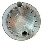
Within the primary architecture of the model, a polymer cylinder, encircled by an intricate grid of 32 electrodes (2 × 16 electrodes), serves as the focal point. This cylinder boasts a diameter measuring ø200 mm. Nestled within the conduit’s confines are two distinct categories of polymer tubules with a diameter of ø20 mm: solid and hollow. The whole cylinder is inundated with tap water, and the conductivity oscillates around 500 μS/cm.
In tomographic imaging, the integrity of the collected data is crucial. Thus, it is vital that all tools involved, including imaging devices, electrode systems, electronic interfaces, and computational methodologies, meet the highest standards. The fidelity of the final images hinges on the excellence of the entire apparatus, underscoring the necessity for stringent technical quality across the board.
2.2. Simulation Environment
Electrical impedance tomography (EIT) is an imaging technique that uses electrical measurements to reconstruct the internal structure of an object. The basic step in EIT is to apply electrodes to the object’s surface through which currents of known value are passed and then the values of the voltages between many pairs of electrodes are measured. By measuring the potential difference between the electrodes, the impedance of the interior of the test area can be estimated. The main challenge of EIT is the so-called inverse problem. By measuring the potentials outside the object, we want to find the impedance values inside the object. The inverse problem arises from having insufficient input data (independent variables) relative to the output variables (observations), leading to ambiguity in the derived solution. In the research presented here, it is important to reconstruct images inside an industrial reactor’s object under study based on capacitance measurements from electrodes placed outside and around the vessel.
Neural networks can be used to solve the inverse problem in EIT. However, to train the network, it is necessary to generate a synthetic dataset. For this purpose, it was necessary to solve the forward problem. The forward problem in EIT refers to the mathematical modelling and computational aspects of predicting the voltages at the electrodes when the distribution of electrical conductivity inside the subject is known. Essentially, given a known conductivity distribution in an area and knowing where the currents are applied, the resulting voltages at the boundary of that area can be determined. In the case of EIT, the forward problem involves determining the potential distribution through Laplace’s partial differential equation, expressed as:
where: —electrical conductivity and —electric potential.
The forward problem involves determining the potential function ∇u based on the given conductivity , where represents the spatial coordinate vector. These calculations consider the boundary conditions under homogeneous conditionswhere σ remains constant.
One approach to solving the conductivity problem in EIT is using Dirichlet-to-Neumann (DtN) mapping. DtN mapping is crucial in many inverse algorithms in EIT, where the goal is to determine the conductivity σ based on potential measurements on the boundary. The DtN map relates the boundary data as Dirichlet conditions (specified potential) to the corresponding normal potential derivatives on the same boundary (corresponding to the current). Mathematically, the DtN map, , is defined as:
where ∂Ω is the boundary of the domain Ω, and n is the normal vector to the boundary.
The solution to the forward problem in EIT is to find the potential u inside Ω based on the known conductivity σ and boundary data. Knowing Λ is akin to understanding the current density distribution resulting from any voltage configuration on the boundary.
To efficiently solve Equation (1) in complex geometries or for irregular conductivity distributions, the finite element method (FEM) is often employed. This method involves dividing the domain into small, simpler sub-domains (so-called finite elements) and approximating the solution in each element, then combining these solutions into a global solution. For Equation (1), an energy functional can be created, which is minimized in the FEM process.
In the context of EIT, the forward problem is adeptly addressed using the finite element method (FEM). This computational technique allows for meticulously determining primary function values across individual elements demarcated in the FEM grid, setting a firm ground for intricate analyses in EIT. The simulation environment was developed by integrating the Eidors toolbox with Matlab 2023a software, a collaboration that enabled the successful implementation of the FEM modelling. Consequently, it enabled the creation of detailed meshes formed from tetrahedral finite elements, commonly known as voxels. Voxel values are related to electrical conductivity but do not represent direct electrical conductivity measurements but “arbitrary units”. It is a device thanks to which it is possible to visualize the inside of the analyzed object based on differences in electrical conductivity.
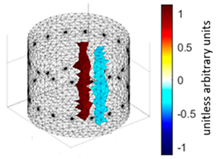
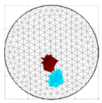
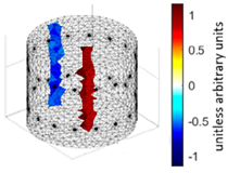
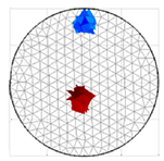
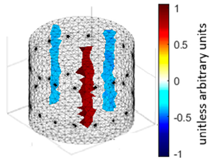
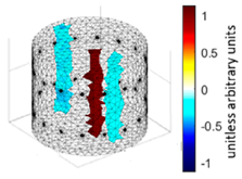
A virtual digital representation of the industrial tank was created, detailing the geometry and material properties of the examined object along with its surrounding electrodes. Central to this model is the spatial grid of finite elements that is the foundation for generating the tomographic image. Using the FEM model, pattern images were created by allocating specific conductivity values to each voxel. Figure 2 shows the nature of EIT’s forward and inverse problems. PVC plastic rods have better conductivity properties than air. Conductivity (σ) is inversely proportional to electrical resistance (R). Using Ohm’s law, electrical resistance can be expressed as:
where L is the length of the conductor, and A is its cross-sectional area. In the visualization, the PVC rod is shown in brown or red, while the hollow pipe is shown in blue. This is according to the color legend (color bar). The finite element values, which are also FEM voxels, are unitless. These are the so-called “arbitrary units”, which are highly correlated with voxel conductance. However, these are not absolute conductance values, which is why EIT is not strictly a measurement method. EIT enables imaging of voxel conductance in relation to the background, which in the examined case is tap water.

Figure 2.
The nature of EIT’s forward and inverse problems.
The finite element method (FEM) has been applied to solve both forward and inverse problems. In addressing the forward problem, a synthetic training dataset was generated. Random tomograms of different inclusion configurations were created on a spatial finite element mesh with 14,100 voxels. The Eidors toolbox was then used to make 448-element measurement vectors corresponding to each reference image. The inverse problem is a key challenge in tomography. Its resolution enables the conversion of measurements into tomographic images. Given that the inverse problem is an “ill-posedness problem” characterized by indeterminacy due to a deficit of input data, no unequivocal solution yields a perfect image on the mesh. The utilization of the method presented in this study aims to enhance the efficacy of the solutions obtained for the inverse problem.
2.3. Network Architecture
The main objective of the research conducted was to optimize the loss function for neural network models used in electrical tomography of industrial reactors. Therefore, it was proposed to train a classifier that, based on measurement data, determines the appropriate loss function to be used. In particular, the classifier suggests which model, integrated with various loss functions, should be implemented to achieve the highest reconstruction quality. A schematic of the conducted research is shown in Figure 3.
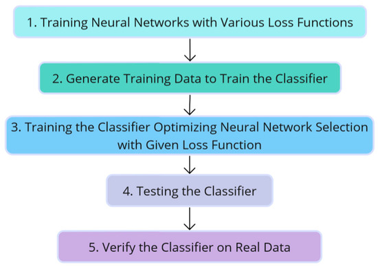
Figure 3.
Diagram of the conducted research.
This research’s first phase involved training neural networks with different loss functions. The trained models are based on a simple LSTM network structure consisting of a single layer with 128 hidden units. As the main objective of this study is not to develop a novel, more efficient neural network structure, a simple LSTM network was chosen. The input layer of the network consists of 448 values. The network was designed to contain 14,100 output channels and was trained using mini-batches of size 64 for 50 epochs. The model was developed using the widely used optimization method called Adaptive Moment Estimation, commonly called ADAM. Further, 5% noise was introduced into the input data. A dataset of 25,958 training cases and 5000 validation cases was used to teach the models.
A custom training loop was used to teach the neural network by changing the loss function. The loss function plays a pivotal role in the training process of a neural network, delineating the discrepancy between the model’s predictions and the actual values. Quantifying this difference is imperative, as it enables the adjustment of the model’s parameters to minimize error and enhance prediction accuracy. Many loss functions exist, each possessing distinct characteristics suitable for diverse problem types. Selecting the appropriate loss function is key to achieving optimal performance of the model under research.
For the analysis, 4 model variants with various loss functions designed for regression problems were used: HMSE, Huber, l1loss and l2loss, shown in Table 1. HMSE, or half mean squared error, represents the average squared differences between predicted and actual values, halved. Relative to the standard MSE, it is computationally simpler and exhibits high sensitivity to errors, which may be advantageous in certain applications. Its main disadvantage is its high susceptibility to outliers, which can lead to over-adaptation to anomalies. The Huber loss is a fusion of MSE for minor discrepancies and MAE for pronounced ones. It boasts a greater resistance to outliers than MSE, demonstrating resilience to data noise. Including an additional parameter, δ, which determines the transition between the two modes, might introduce complexity in the model selection process but offers greater adaptability to varying circumstances. L1 loss, known as mean absolute error (MAE), calculates the average absolute differences between predictions and actual values. It is notably robust against outliers and computationally straightforward. However, it may not be as accurate as MSE when data are well fitted to a quadratic function.

Table 1.
Analyzed loss functions.
Conversely, L2 loss or mean squared error (MSE) displays a heightened sensitivity to discrepancies and provides insight into the model’s fit quality. However, its sensitivity to outliers might induce overfitting to exceptional values. Selecting an appropriate loss function is critical to achieving optimal model performance. Analyzing and conducting experimental studies with different loss functions in the context of a specific problem is key to identifying the most effective solution.
The peak signal-to-noise ratio (PSNR), calculated according to the equation, was used to evaluate the quality of the resulting reconstruction models:
where: peakval is the total number of voxels in the 3D image, and MSE is the mean squared error between the predicted value from the network and the target value.
The PSNR index was chosen to analyze the image reconstruction quality because it directly relates to the mean squared error (MSE). When the MSE is low, indicating little difference between images, the PSNR value is high, indicating better reconstruction quality. PSNR provides an intuitive image quality assessment, considering the maximum signal power versus noise power. It is an indicator that can be easily compared with the results of other methods. Moreover, its scalability allows it to be easily adapted to different image resolutions and formats, and its computational simplicity guarantees efficiency in practical applications, especially when analyzing large datasets.
In the research, the Huber loss function was meticulously studied over a range of δ values from 0.1 to 1.0 (default value in Matlab), with an incremental step of 0.1. After an extensive evaluation with 1000 test cases and evaluation of the reconstruction quality using the PSNR metric, it was found that the optimal result was obtained for δ = 0.1. Specifically, the highest reconstruction quality was manifested in 282 cases out of 1000, as illustrated in Figure 4. Based on these results, the network was trained using the Huber loss function with an optimal δ value of 0.1.
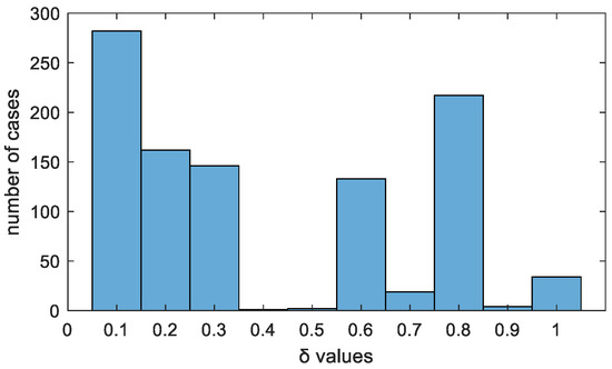
Figure 4.
Best reconstruction quality for various δ values.
The second stage of the research conducted was to generate training data to train the classifier. The data were generated using the following procedure:
- Measured data were input, and trained models using various loss functions—MSE, Huber, l1loss and l2loss—were imported.
- For each case in the dataset, image reconstructions were predicted using all four models.
- For each case and for each model, the PSNR between the predicted output and the based target was computed.
- For each case, the model with the highest PSNR value was selected.
- The index of the optimal model for each case was then recorded in a designated array.
The resulting array and measurement data provide a set of inputs and outputs for training the classifier. The training data generation to train the classifier was carried out on a base of 5000 cases, different from those used to train previous models.
The next stage of the conducted research was to train a classifier that, based on the measurement data, allows the determination of which trained models should be used to perform image reconstruction. The classifier will return the index of the model that should be used for reconstruction (Table 2). The Classification Learner toolbox was employed within MATLAB, an integral component of the Machine Learning and Deep Learning toolbox for classifier training. A comprehensive analysis was undertaken to utilize all the models available within this toolbox, including Decision Trees, Discriminant Analysis, support vector machines (SVMs), K-Nearest Neighbors (KNN), Ensemble Classifiers, Logistic Regression, Neural Networks, and Naive Bayes. Ten-fold cross-validation was meticulously applied to ensure robustness and reliability in the model evaluations.

Table 2.
Model description.
After training the classifier, it was tested on a sample of 1000 cases. Subsequently, the classifier’s performance was validated using real-world data. These real data were sourced from the research setup described in Section 2.1 (Figure 1), which was developed in the Netrix S.A. laboratory.
3. Results and Discussion
As a result of training the classifier, the best results were obtained for support vector machines (SVMs) with multi-class one-vs-one classification, for which validation accuracy was achieved at 59.6%. The achieved model accuracy of 59.6% is neither exceptionally high nor particularly low. For a problem with four classes, random classification would yield a probability of 25%. The model’s accuracy of 59.6% is much better than randomness.
The diagram illustrating the operation of the entire system optimizing the selection of the loss function is shown in Figure 5. The SVM classifier selects the most optimal neural network based on the measurement vector with a selected loss function. In the next step, image reconstruction is carried out using the selected neural network.

Figure 5.
Diagram of the operation of the system optimizing the selection of loss function.
Results of the reconstructions obtained using four neural network variants with various loss functions, HMSE, Huber, l1loss, and l2loss, as well as the results from the trained classifier, are presented in Table 3. This study was based on synthetically generated datasets, as reference images are essential in the learning process and the assessment of only reconstruction accuracy for such data.

Table 3.
Results of the reconstructions using models with various loss functions.
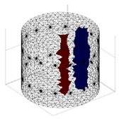
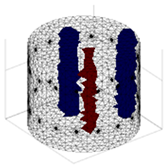
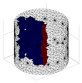
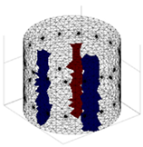
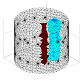
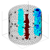
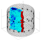
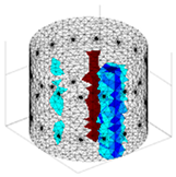
Four representative cases were selected for comparison and are shown in an isometric view. The columns present the cases analyzed. The first row shows reference images, and the following rows show reconstructions using the following methods in the following order: HMSE, Huber, l1loss, and l2loss. The last line presents reconstructions using the model obtained from the classifier operation. By analyzing the obtained reconstructions, it is possible to evaluate the performance of the classifier in optimizing the loss function. The worst results were obtained in each case analysis using the l1loss loss function. It is worth noting that the classifier considered this method optimal in none of the cases studied. In case #1, visual analysis of the reconstruction suggests that the reconstruction using the Huber loss function is closest to the original reference image, an observation consistent with the choice of the classifier. In case #2 and case #3, all reconstructions (except the one obtained using l1loss) are so close to the pattern that it is difficult to determine their quality based on visual observation alone unambiguously. A similar situation occurs in case #4, where the reconstructions with the HMSE and l2loss loss functions are very close to the pattern. In cases #2 to #4, the classifier identified the model based on the l2loss loss function as the most optimal for reconstruction.
In order to deepen the analysis of the received reconstructions and to evaluate the subjective evaluation performed above, an analysis was performed using three quality indicators. One is PSNR, which was previously used to select the most optimal model when generating data for training the classifier. The second indicator is the mean squared error (MSE), calculated according to the formula:
where: R—the total count of voxels in the 3D image, —the i-th voxel of the pattern image, and —the i-th voxel of the reconstructed image.
In these studies, the image correlation coefficient (ICC) was also employed as a measurement. It is determined using Equation (6):
where is the average voxel value of the pattern image and is the average voxel value of the reconstructed image.
Table 4 shows the values of the image quality indicators: PSNR, ICC, and MSE for four representative cases and the average of 1000 validation cases. The analysis of these indicators for case #1 confirms the previous subjective and qualitative assessments based on the analysis of the images in Table 3. For cases #2 to #4, the quality indicators indicate that the highest reconstruction quality was achieved for the model with the l2loss loss function. This observation is consistent with the classifier’s results, proving its accurate performance. This support complements the subjective interpretations resulting from the analysis of Table 3. However, when analyzing the quality indicators for the average of 1000 validation cases, the best results were obtained from the classifier’s operation optimizing the neural model’s loss function.

Table 4.
Comparison of reconstruction quality indicators.
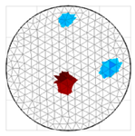
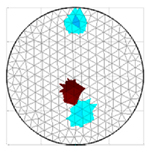
Reconstructions based on the actual measurements are shown in Table 5. Color calibration was performed during the reconstruction. These are five cases for different configurations of the number and position of the tubes in the water inside the reactor model. In the first column are photos of the studied objects taken from above, which allows us to determine the position of the tubes relative to the bottom. The next column presents reconstructions of the axonometric view (3D). Above the reconstruction image is information about the model (loss function) with which it was made (see Table 2). The last column shows the reconstruction in the top view, so that a comparison can be made between the obtained results and the real data. As the results indicate, the reconstructions obtained coincide with the real objects. In some cases, the shape of the tubes is not fully reproduced, but this may be due to noise in the measurement data. The data used to train the LSTM network with various loss functions were noisy at the level of 5%, but in real conditions, such noise may have different parameters, which may result in the obtained quality of the reconstructions.

Table 5.
Reconstructions based on real measurements.
4. Conclusions
The main aim of this research was to analyze the loss functions for neural network models used in electrical tomography of industrial reactors in terms of their operation and energy optimization. As a solution, a classifier was designed to recommend the optimal loss function based on the measurement data. This classifier suggests which model, connected with different loss functions, should be used to ensure the best reconstruction quality. Significantly, implementing this classifier is anticipated to increase the maintenance energy efficiency and the reliability of industrial reactors by facilitating more accurate and data-driven reconstructions. The method marks a significant shift from conventional practices to a more systematic, data-driven approach.
Four models based on a simple LSTM network structure with various loss functions were initially trained to achieve HMSE, Huber (δ = 0.1), l1loss, and l2loss. Then, training data were generated to train a classifier, which was trained and tested. The best classifier training results were for support vector machines (SVMs). The quality of the obtained reconstructions was evaluated using three image quality indicators: PSNR (peak signal-to-noise ratio), ICC (image correlation coefficient), and MSE (mean squared error). The classifier results for individual cases from Case #1 to Case #4 and the average of 1000 validation cases demonstrate its effective operation. For each case, the classifier accurately identified the most suitable model with the optimal loss function, ensuring the highest quality of image reconstructions. This was evident in the comparative analysis of the PSNR, ICC, and MSE values across different loss functions (HMSE, Huber, l1loss, and l2loss) and the selections made by the classifier.
The classifier’s performance was validated using real data consisting of a measurement vector of 448 values. Upon applying this classifier to actual measurements from the Netrix S.A. laboratory, the resulting reconstructions closely matched the real objects. Any minor variations observed could be due to noise in the data.
The classifier’s ability to navigate through different loss functions and recommend the most appropriate one based on the specific characteristics of each case contributes significantly to the optimization of neural network models in electrical tomography. This not only increases the accuracy and reliability of the reconstructions, but also implies potential improvements in energy efficiency and maintenance of industrial reactors. The classifier can serve as a powerful tool for data-driven decision making, reducing the trial-and-error approach traditionally associated with the model and loss function selection in industrial applications.
The findings of this study suggest that the application of the classifier could revolutionize the maintenance and operation of industrial reactors. By enabling more precise and efficient reconstructions, the classifier not only boosts energy efficiency but also contributes to safer and more reliable industrial operations. This advancement is particularly relevant in the context of the growing need for energy conservation and operational efficiency in industrial sectors.
Author Contributions
Conceptualization, M.K., G.K. and T.R.; investigation, G.K.; resources, T.R. and K.G.; data curation, K.G. and W.C.; writing—original draft preparation, M.K. and G.K.; writing—review and editing, T.R. and J.S.; visualization, M.K.; supervision, T.R., J.S. and W.C.; project administration, M.K. All authors have read and agreed to the published version of the manuscript.
Funding
This research received no external funding.
Data Availability Statement
Dataset available on request from the authors.
Conflicts of Interest
Author Tomasz Rymarczyk was employed by the company Research & Development Centre, Netrix S.A. The remaining authors declare that the research was conducted in the absence of any commercial or financial relationships that could be construed as a potential conflict of interest.
References
- Gholami, Z.; Gholami, F.; Tišler, Z.; Vakili, M. A Review on the Production of Light Olefins Using Steam Cracking of Hydrocarbons. Energies 2021, 14, 8190. [Google Scholar] [CrossRef]
- Silva, D.P.; Brányik, T.; Dragone, G.; Vicente, A.A.; Teixeira, J.A.; Almeida, E.; Silva, J.B. High Gravity Batch and Continuous Processes for Beer Production: Evaluation of Fermentation Performance and Beer Quality. Chem. Pap. 2008, 62, 34–41. [Google Scholar] [CrossRef]
- Aguirre-Ezkauriatza, E.J.; Galarza-González, M.G.; Uribe-Bujanda, A.I.; Ríos-Licea, M.; López-Pacheco, F.; Hernández-Brenes, C.M.; Alvarez, M.M. Effect of Mixing During Fermentation in Yogurt Manufacturing. J. Dairy. Sci. 2008, 91, 4454–4465. [Google Scholar] [CrossRef] [PubMed]
- Vilkhu, K.; Mawson, R.; Simons, L.; Bates, D. Applications and Opportunities for Ultrasound Assisted Extraction in the Food Industry—A Review. Innov. Food Sci. Emerg. Technol. 2008, 9, 161–169. [Google Scholar] [CrossRef]
- Reis, M.S.; Gins, G.; Chiang, L.H.; Braatz, R.D. Industrial Process Monitoring in the Big Data/Industry 4.0 Era: From Detection, to Diagnosis, to Prognosis. Processes 2017, 5, 35. [Google Scholar] [CrossRef]
- Shu, X.; Zhang, S.; Li, Y.; Chen, M. An Anomaly Detection Method Based on Random Convolutional Kernel and isolation Forest for Equipment State Monitoring. Eksploat. I Niezawodn.–Maint. Reliab. 2022, 24, 758–770. [Google Scholar] [CrossRef]
- Gu, D.; Nie, R.; Han, W.; Chen, G.; Jia, L. Research on Preventive Maintenance Strategy of Coating Machine Based on dynamic Failure Rate. Eksploat. I Niezawodn.–Maint. Reliab. 2023, 25, 2023. [Google Scholar] [CrossRef]
- Steinmann, A.; Finger, M.; Nowacki, C.; Decembrino, D.; Hubmann, G.; Girhard, M.; Urlacher, V.B.; Lütz, S. Heterologous Lignan Production in Stirred-Tank Reactors—Metabolomics-Assisted Bioprocess Development for an In Vivo Enzyme Cascade. Catalysts 2022, 12, 1473. [Google Scholar] [CrossRef]
- Jiang, Y.; Yin, S.; Kaynak, O. Performance Supervised Plant-Wide Process Monitoring in Industry 4.0: A Roadmap. IEEE Open J. Ind. Electron. Soc. 2021, 2, 21–35. [Google Scholar] [CrossRef]
- Resende, C.; Folgado, D.; Oliveira, J.; Franco, B.; Moreira, W.; Oliveira-Jr, A.; Cavaleiro, A.; Carvalho, R. TIP4.0: Industrial Internet of Things Platform for Predictive Maintenance. Sensors 2021, 21, 4676. [Google Scholar] [CrossRef] [PubMed]
- Keleko, A.T.; Kamsu-Foguem, B.; Ngouna, R.H.; Tongne, A. Artificial Intelligence and Real-Time Predictive Maintenance in Industry 4.0: A Bibliometric Analysis. AI Ethics 2022, 2, 553–577. [Google Scholar] [CrossRef]
- Hashemian, H.M. State-of-the-Art Predictive Maintenance Techniques. IEEE Trans. Instrum. Meas. 2011, 60, 226–236. [Google Scholar] [CrossRef]
- Dutz, F.J.; Heinrich, A.; Bank, R.; Koch, A.W.; Roths, J. Fiber-Optic Multipoint Sensor System with Low Drift for the Long-Term Monitoring of High-Temperature Distributions in Chemical Reactors. Sensors 2019, 19, 5476. [Google Scholar] [CrossRef]
- Rymarczyk, T.; Kłosowski, G. Innovative Methods of Neural Reconstruction for Tomographic Images in Maintenance of Tank Industrial Reactors. Eksploat. I Niezawodn. 2019, 21, 261–267. [Google Scholar] [CrossRef]
- Kłosowski, G.; Rymarczyk, T.; Niderla, K.; Kulisz, M.; Skowron, Ł.; Soleimani, M. Using an LSTM Network to Monitor Industrial Reactors Using Electrical Capacitance and Impedance Tomography—A Hybrid Approach. Eksploat. I Niezawodn.–Maint. Reliab. 2023, 25, 11. [Google Scholar] [CrossRef]
- Mosorov, V.; Rybak, G.; Sankowski, D. Plug Regime Flow Velocity Measurement Problem Based on Correlability Notion and Twin Plane Electrical Capacitance Tomography: Use Case. Sensors 2021, 21, 2189. [Google Scholar] [CrossRef] [PubMed]
- Wanta, D.; Makowiecka, O.; Smolik, W.T.; Kryszyn, J.; Domański, G.; Midura, M.; Wróblewski, P. Numerical Evaluation of Complex Capacitance Measurement Using Pulse Excitation in Electrical Capacitance Tomography. Electronics 2022, 11, 1864. [Google Scholar] [CrossRef]
- Wanta, D.; Smolik, W.T.; Kryszyn, J.; Midura, M.; Wróblewski, P. Image Reconstruction Using Z-Axis Spatio-Temporal Sampling in 3D Electrical Capacitance Tomography. Meas. Sci. Technol. 2022, 33, 114007. [Google Scholar] [CrossRef]
- Ye, Z.; Banasiak, R.; Soleimani, M. Planar Array 3D Electrical Capacitance Tomography. Insight Non-Destr. Test. Cond. Monit. 2013, 55, 675–680. [Google Scholar] [CrossRef]
- Dalton, L.E.; Räsänen, M.; Voss, A.; Seppänen, A.; Pourghaz, M. Investigating the Use of Electrical Capacitance Tomography to Image Rapid Transient Moisture Flow through Cracks in Concrete. Cem. Concr. Compos. 2023, 140, 105070. [Google Scholar] [CrossRef]
- Rasel, R.K.; Chowdhury, S.M.; Marashdeh, Q.M.; Teixeira, F.L. Review of Selected Advances in Electrical Capacitance Volume Tomography for Multiphase Flow Monitoring. Energies 2022, 15, 5285. [Google Scholar] [CrossRef]
- Zhang, Y.; Chen, D. Electrical Capacitance Tomography and Parameter Prediction Based on Particle Swarm Optimization and Intelligent Algorithms. Wirel. Netw. 2021, 2021, 1–12. [Google Scholar] [CrossRef]
- Jaiswal, R.; Moldestad, B.M.E.; Eikeland, M.S.; Nielsen, H.K.; Thapa, R.K. Image Processing and Measurement of the Bubble Properties in a Bubbling Fluidized Bed Reactor. Energies 2022, 15, 7828. [Google Scholar] [CrossRef]
- Tang, Y.; Lin, W.; Xiao, S.; Tang, K.; Lin, X. A Measurement Compensation Method for Electrical Capacitance Tomography Sensors with Inhomogeneous Electrode Parameters. Electronics 2022, 11, 2957. [Google Scholar] [CrossRef]
- Duraj, A.; Korzeniewska, E.; Krawczyk, A. Classification Algorithms to Identify Changes in Resistance. Prz. Elektrotechniczny 2015, 1, 80–83. [Google Scholar] [CrossRef]
- Dusek, J.; Mikulka, J. Measurement-Based Domain Parameter Optimization in Electrical Impedance Tomography Imaging. Sensors 2021, 21, 2507. [Google Scholar] [CrossRef] [PubMed]
- Liu, S.; Huang, Y.; Wu, H.; Tan, C.; Jia, J. Efficient Multitask Structure-Aware Sparse Bayesian Learning for Frequency-Difference Electrical Impedance Tomography. IEEE Trans. Ind. Inf. 2021, 17, 463–472. [Google Scholar] [CrossRef]
- Ricard, F.; Brechtelsbauer, C.; Xu, X.Y.; Lawrence, C.J. Monitoring of Multiphase Pharmaceutical Processes Using Electrical Resistance Tomography. Chem. Eng. Res. Des. 2005, 83, 794–805. [Google Scholar] [CrossRef]
- Szczęsny, A.; Korzeniewska, E. Selection of the Method for the Earthing Resistance Measurement. Prz. Elektrotechniczny 2018, 94, 178–181. [Google Scholar] [CrossRef]
- Yu, H.; Wan, X.; Dong, Z.; Zhang, Z.; Jia, J. Estimation of Reference Voltages for Time-Difference Electrical Impedance Tomography. IEEE Trans. Instrum. Meas. 2022, 71, 4506710. [Google Scholar] [CrossRef]
- Zhu, Z.; Li, G.; Luo, M.; Zhang, P.; Gao, Z. Electrical Impedance Tomography of Industrial Two-Phase Flow Based on Radial Basis Function Neural Network Optimized by the Artificial Bee Colony Algorithm. Sensors 2023, 23, 7645. [Google Scholar] [CrossRef]
- Wang, J. An Efficient One-Step Proximal Method for EIT Sparse Reconstruction Based on Nonstationary Iterated Tikhonov Regularization. Appl. Math. Sci. Eng. 2023, 31, 2157413. [Google Scholar] [CrossRef]
- Kieu, D.T.; Vu, H.D.; Nguyen, T.T.H.; Nguyen, T.T. Applying Electrical Impedance Tomography Techniques for Detection of Decay Inside Trees. Inżynieria Miner. 2021, 1, 31–40. [Google Scholar] [CrossRef]
- Kłosowski, G.; Rymarczyk, T.; Niderla, K. Use of the Two-Stage Neural System in Electrical Impedance Tomography for Imaging Moisture inside Walls. In Proceedings of the SenSys 2022—Proceedings of the 20th ACM Conference on Embedded Networked Sensor Systems, Boston, MA, USA, 6–9 November 2022; pp. 861–862. [Google Scholar] [CrossRef]
- Neves, F.d.O.; Ewbank, H.; Roveda, J.A.F.; Trianni, A.; Marafão, F.P.; Roveda, S.R.M.M. Economic and Production-Related Implications for Industrial Energy Efficiency: A Logistic Regression Analysis on Cross-Cutting Technologies. Energies 2022, 15, 1382. [Google Scholar] [CrossRef]
- Rehman, S.U.; Tu, S.; Huang, Y.; Rehman, O.U. A Benchmark Dataset and Learning High-Level Semantic Embeddings of Multimedia for Cross-Media Retrieval. IEEE Access 2018, 6, 67176–67188. [Google Scholar] [CrossRef]
- Rehman, S.U.; Huang, Y.; Tu, S.; Ahmad, B. Learning a Semantic Space for Modeling Images, Tags and Feelings in Cross-Media Search. Lect. Notes Comput. Sci. (Incl. Subser. Lect. Notes Artif. Intell. Lect. Notes Bioinform.) 2019, 11607, 65–76. [Google Scholar] [CrossRef]
- Cao, Y.; Gu, Q. Generalization Error Bounds of Gradient Descent for Learning Over-Parameterized Deep ReLU Networks. Proc. AAAI Conf. Artif. Intell. 2020, 34, 3349–3356. [Google Scholar] [CrossRef]
- Kim, Y.; Park, H. Deep Learning-Based Automated and Universal Bubble Detection and Mask Extraction in Complex Two-Phase Flows. Sci. Rep. 2021, 11, 8940. [Google Scholar] [CrossRef]
- Botchkarev, A. A New Typology Design of Performance Metrics to Measure Errors in Machine Learning Regression Algorithms. Interdiscip. J. Inf. Knowl. Manag. 2019, 14, 45–76. [Google Scholar] [CrossRef]
- Qi, J.; Du, J.; Siniscalchi, S.M.; Ma, X.; Lee, C.H. On Mean Absolute Error for Deep Neural Network Based Vector-to-Vector Regression. IEEE Signal Process Lett. 2020, 27, 1485–1489. [Google Scholar] [CrossRef]
- Pawlik, P.; Kania, K.; Przysucha, B. Fault Diagnosis of Machines Operating in Variable Conditions Using Artificial Neural Network Not Requiring Training Data from a Faulty Machine. Eksploat. I Niezawodn.–Maint. Reliab. 2023, 25, 168109. [Google Scholar] [CrossRef]
- Qin, C.; Li, Y.; Liu, C.; Ma, X. Cuff-Less Blood Pressure Prediction Based on Photoplethysmography and Modified ResNet. Bioengineering 2023, 10, 400. [Google Scholar] [CrossRef] [PubMed]
Disclaimer/Publisher’s Note: The statements, opinions and data contained in all publications are solely those of the individual author(s) and contributor(s) and not of MDPI and/or the editor(s). MDPI and/or the editor(s) disclaim responsibility for any injury to people or property resulting from any ideas, methods, instructions or products referred to in the content. |
© 2024 by the authors. Licensee MDPI, Basel, Switzerland. This article is an open access article distributed under the terms and conditions of the Creative Commons Attribution (CC BY) license (https://creativecommons.org/licenses/by/4.0/).
