Assessing the Reliability and Optimizing Input Parameters of the NWP-CFD Downscaling Method for Generating Onshore Wind Energy Resource Maps of South Korea

Abstract

The numerical weather prediction (NWP) method is one of the popular wind resource forecasting methods, but it has the limitation that it does not consider the influence of local topography. The NWP-CFD downscaling considers topographic features and surface roughness by performing computational fluid dynamics (CFD) with the meteorological data obtained by the NWP method as a boundary condition. The NWP-CFD downscaling is expected to be suitable for wind resource forecasting in Korea, but it lacks a quantitative evaluation of its reliability. In this study, we compare the actual measured data, the NWP-based data, and the NWP-CFD-based data quantitatively and analyze the three main input parameters used for the calculation of NWP-CFD (minimum vertical grid size Δz_min, the difference angle Δdir, and the forest model activation reference length l₀). Compared to the actual measurement data, the NWP-based data overestimate wind resources by more than 35%, while the NWP-CFD-based data show an error of about 8.5%. The Δz_min and Δdir have little effect on the results, but the l₀ has a large effect on the simulation results, and it is necessary to adjust the values appropriately corresponding to the characteristics of an area.

1. Introduction

As concerns about environmental problems increase, interest in renewable energy that can replace fossil energy is rising. The development and utilization of renewable energy sources are rapidly growing worldwide, and the total generation of renewable energy reached 3.17 × 108 toe as of 2014 [1,2]. Wind energy accounts for a large share of various renewable energies, accounting for 52% of global renewable energy use in 2017 [3,4]. Korea is also expanding its renewable energy operation. As of 2020, new and renewable energy generation amounted to about 43,000 GWh, accounting for 7.43% of the total generation. Among them, wind energy generation accounted for 7.3%, an increase of 17.6% compared to the previous year [5].

Since the amount of power generated by a wind turbine is affected by wind resources in the installation area, accurate wind resource forecasting is essential in selecting a wind farm site [6,7]. The numerical weather prediction (NWP) method predicts future weather conditions based on current weather conditions by solving numerical models of the atmosphere and oceans. It spatially discretizes the Earth’s atmosphere and solves the partial differential equations that govern the atmosphere, requiring a significant computational source. Many researchers have utilized meteorological data predicted by the NWP method to assess wind resources [8,9]. It is also used in Korea for aviation and military purposes [10,11]. The sole NWP method, however, has limitations to be used in assessing the wind resources of a specific site: a low spatial resolution of the obtained meteorological data due to a high computing cost and the inability to consider the impact of regional topographical characteristics on wind distributions. In Korea, most of the onshore wind farms are located in mountainous areas with complex topography, and there is a risk of overestimating wind speed and energy production when assessed using meteorological data from the sole NWP method.

To overcome the limitations of NWP, the NWP-CFD downscaling method was used [12,13,14], where the meteorological data from the NWP method were used as boundary conditions to perform CFD simulations. They can increase the spatial resolution of the wind resource map while considering the effect of topographical characteristics and surface roughness on the wind distribution. Thus, the coupled NWP-CFD downscaling method is expected to be more suitable for wind resource forecasting in Korea than the sole NWP method. Che et al. [13] downscaled the Weather Research and Forecasting (WRF) data from a horizontal resolution of 500 m to 100 m and 50 m by coupling the data with CFD simulations implemented by OpenFoam in a mountainous area of Japan. This resulted in improved performance compared to the model using WRF alone. Similarly, Durán et al. [14] increased the spatial resolution of WRF data by coupling the data with CFD simulations using WindSim, which showed improvements in wind speed prediction. Although previous studies [12,13,14] demonstrated that the coupling method surpasses the WRF-alone model in predicting wind data and can increase the spatial resolution of the original data, they have not detailed the effects of crucial parameters such as wind direction resolution and the activation length of the forest model that should be set prior to the coupling simulation on the prediction performance.

Recently, the wind resource map was established for the entire onshore region of South Korea, and the spatial resolution was enhanced from 1 km to 100 m by using the NWP-CFD coupled method [15]. Compared to the data predicted by the NWP method, the wind resource map produced from the coupled method showed an overall decrease in energy production, and this tendency was more prominent in mountainous areas [15]. The high computational cost makes it challenging to assess and optimize the fit of critical input parameters in the coupled simulation, and there is still a lack of relevant research in this area.

The objective of the present study is to suggest quantitative verifications of the NWP-CFD method through comparisons with actual measurement data and to analyze the effects of the input parameters, such as the wind direction resolution, activation length of the forest model, and spatial grid resolution on the wind resources. The following section introduces the data used in the present study. Section 2 briefly explains the coupled NWP-CFD method, and Section 3 and Section 4 present the numerical results. The conclusions are suggested in Section 5.

2. NWP-CFD Coupled Method

2.1. NWP-CFD Downscaling Procedure

The overall computational process aligns with the methodology employed in the prior study [15]. Meteodyn v1.6.2.0, a CFD-based software, is used for the numerical simulation. Figure 1 illustrates the overall procedure of the NWP-CFD coupled method, which downscales mesoscale data from a spatial resolution of 1 km to 100 m. Initially, the CFD simulation is conducted using surface elevation and roughness data across different directions. This process yields the directional speed-up factor, as depicted in Figure 1a,b. Subsequently, the speed-up factor is integrated with the mesoscale data to generate the Weibull coefficients, shown in Figure 1c,d. Finally, by combining these Weibull coefficients with wind turbine power data, the annual energy production (AEP) is calculated, as presented in Figure 1e,f. Section 2.2 introduces the mesoscale data combined into the CFD simulation. Section 2.3 details the setup of the computational domain and the pre-processing procedures. The governing equations, the turbulence model, and the forest model used in the CFD process are comprehensively explained in Section 2.4. Based on the meteorological data derived from the NWP-CFD downscaling method, the annual average wind speed and AEP are calculated. The post-processing procedures related to this calculation are discussed in Section 2.5.

2.2. WRF-Based Mesoscale Meteorological Data

The Korea Institute of Energy Research (KIER) created KIER-WindMap in 2010: a numerical weather prediction (NWP)-based forecast meteorological dataset employed for the NWP-CFD downscaling method. The dataset was generated using the WRF model: a numerical weather forecasting tool utilized for wind resource prediction. This dataset encompasses information like wind speed, wind direction, and humidity at various altitudes (10 m, 40 m, 80 m, 120 m, and 320 m). The dataset has a temporal resolution of one hour and a spatial resolution of 1 km. Figure 2 depicts the time history of the annual wind speed, annual wind speed distribution, and annual wind speed density function at an elevation of 80 m for the location nearest the actual data collection point (at latitude and longitude coordinates 37.73031, 128.69641). The average annual wind speed and the annual energy production (AEP) are predicted to be 8.1 m/s and 13,178 MW, respectively.

2.3. Computaional Domain and Pre-Processing Procedure of CFD

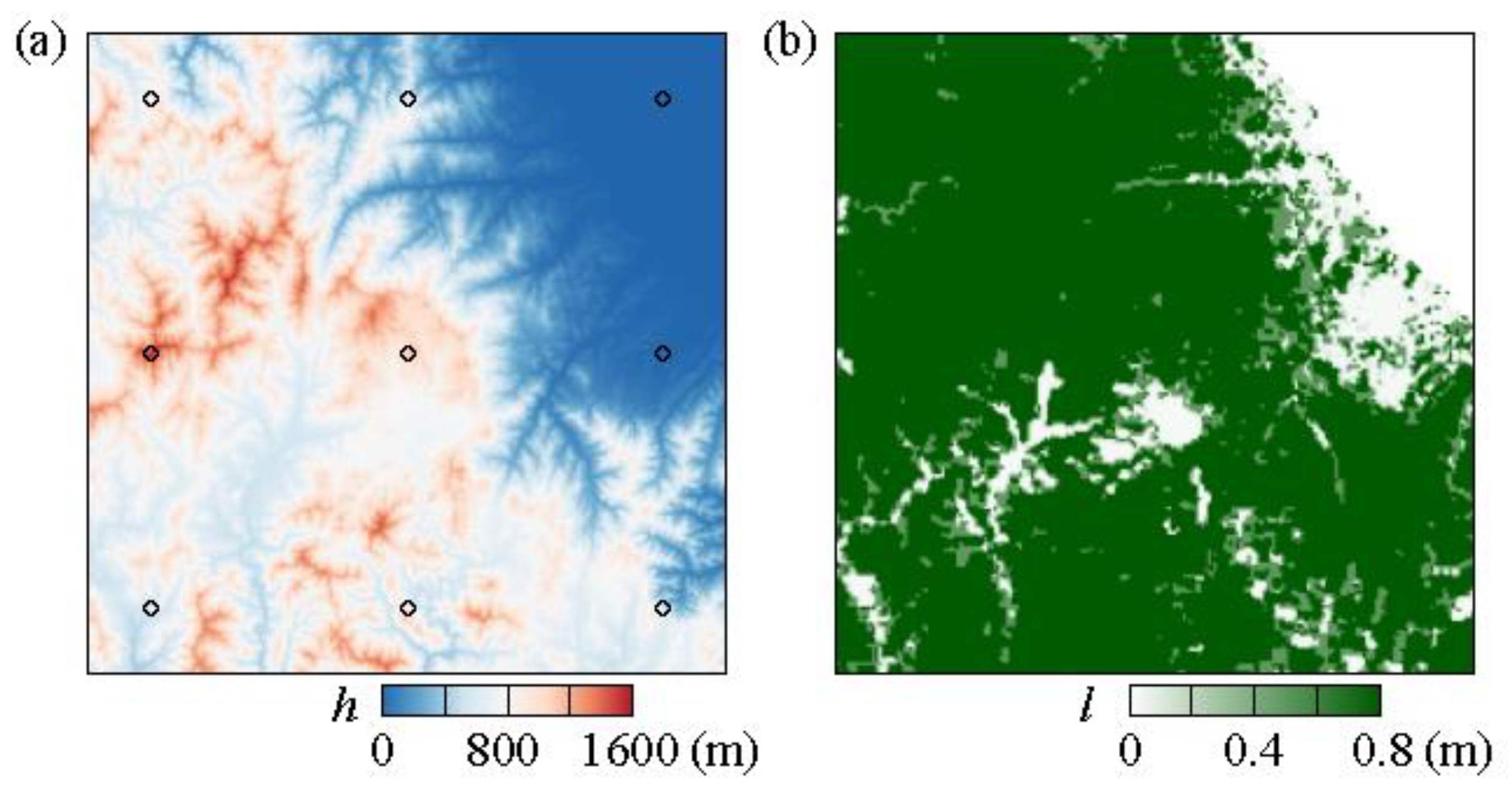
A 50 km × 50 km computational area is established, with the actual measurement location at its center. Figure 3 indicates the extent of this computation area for a quantitative comparison with the real measurement data. This computational domain is presented in terms of UTM zone 52n coordinates. To account for local features and forest surface roughness, a digital elevation model (DEM) and land cover data are required. These data are visually depicted in Figure 4a,b.

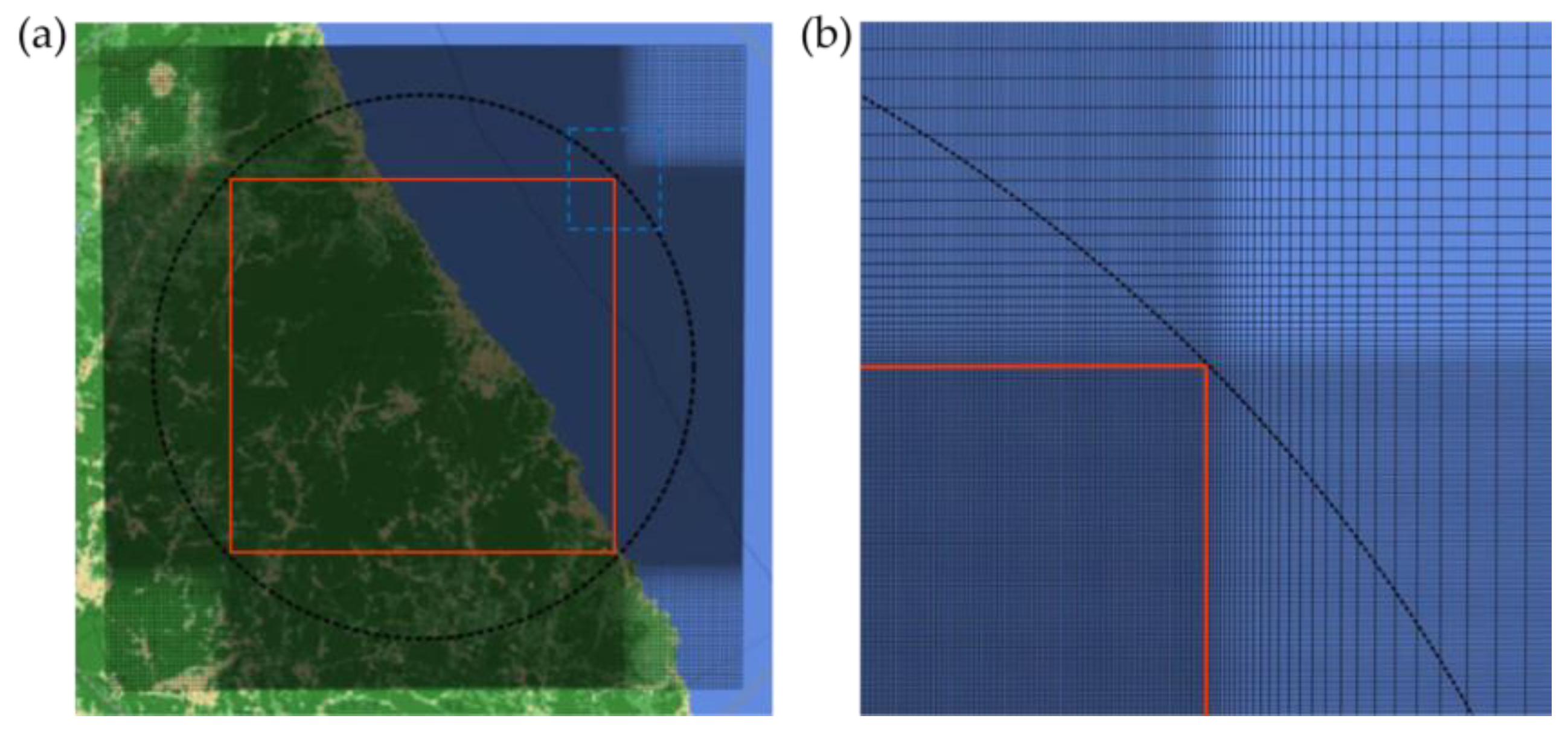
The simulation takes into account the effects of wind blowing from various directions by setting a different angle (Δdir) for each direction. Calculations are carried out at intervals of 15°, 30°, and 45° to ascertain the impact of the difference angle on the calculation result. Figure 5 shows the horizontal grid system in the computational domain as depicted in Figure 3. The thin black solid line denotes the grids in Figure 5a. The thick black dashed line and red solid line correspond to those in Figure 3. Figure 5b shows the magnified view of the horizontal grids in the region denoted by the blue dashed line, where the horizontal grid has a 100 m spatial resolution inside the red solid line, and the remainder of the domain employs relatively more coarse grids to minimize the computational cost. The horizontal grid resolution matches the wind resource map’s resolution. The vertical grid size is smallest near the surface and less dense at higher elevations. To investigate how the minimum vertical grid size (Δz_min) influences the simulation outcomes, comparisons are made using the Δz_min values of 5.0 m, 7.5 m, and 10 m, in Section 3.1.

2.4. Computational Fluid Dynamics

To obtain the directional wind speed-up factor in the CFD simulation, various boundary conditions are applied. The vertical wind profile is used as the inlet boundary condition, the no-slip condition is applied at the bottom, the symmetric boundary condition is set on the side, and the pressure boundary condition is set at the outlet [15]. The symmetric boundary condition ensures that physical quantities and their first derivatives are identical on both sides of the boundary, with no normal flows to the boundary. This boundary condition helps reduce boundary effects by ensuring that the behavior at the boundary mirrors that in a larger domain. The actual physical system extends beyond the boundaries of the current model, which are not of primary interest to the study. Therefore, the effect of an extended domain is mimicked without actually modeling the entire region, by introducing the symmetric boundary condition on the sides of the computational domain.

The CFD simulation is conducted in the 3-dimensional computational domain to obtain wind speed-up factors at various heights. The flow is governed by the incompressible Navier–Stokes equations, which consist of a set of equations for momentum conservation and mass conservation, respectively, expressed as

$$\begin{array}{c}\frac{\partial \left(\rho u_i\right)}{\partial t}=-\frac{\partial \left(\rho u_i{u}_j\right)}{\partial x_j}-\frac{\partial p}{\partial x_j}+\frac{\partial }{\partial x_j}\left[\mu \left(\frac{\partial u_i}{\partial x_j}+\frac{\partial u_j}{\partial x_i}\right)\right]+F_V,\\ \frac{\partial \rho u_i}{\partial x_i}=0,\end{array}$$

(1)

where ρ denotes the fluid density, u_i is the flow velocity in the i-th direction, t is the time, x is the spatial coordinate, μ is the fluid viscosity, and F_v is the volumetric force. Upon separating the instantaneous flow velocity into its time-averaged and velocity fluctuation components and then applying a time average, the Reynolds Averaged Navier–Stokes (RANS) equation can be derived as,

$$\begin{array}{c}-\frac{\partial \left(\rho \overline{u_i}\overline{u_j}\right)}{\partial x_j}-\frac{\partial \overline{P}}{\partial x_j}+\frac{\partial }{\partial x_j}\left[\mu \left(\frac{\partial {\overline{u}}_i}{\partial x_j}+\frac{\partial {\overline{u}}_j}{\partial x_i}\right)-\rho \overline{{u_i}^{\prime }{u_j}^{\prime }}\right]+F_i=0,\\ \frac{\partial \rho \overline{u_i}}{\partial x_i}=0,\end{array}$$

(2)

where the superscript bar indicates the time-averaged quantities, and u_i’ is the velocity fluctuating component in the i-th direction, and $\rho \overline{{u_i}^{\prime }{u_j}^{\prime }}$ is the turbulent shear stress. A false time step relaxation method is used to iteratively approach a steady-state solution by introducing a ‘false time step’, which is set to 500 in the present study. The transition from the initial state to the steady state is gradually achieved by a relaxation factor of 0.3. This allows the solution to evolve slowly towards the steady state.

To close Equation (2), the Boussinesq assumption is employed, wherein the turbulent shear stress is assumed to be proportional to the gradient of the mean velocity. The corresponding model for eddy viscosity is then expressed as,

$$-\rho \overline{{u_i}^{\prime }{u_j}^{\prime }}=v_T\left(\frac{\partial \overline{u_i}}{\partial x_j}+\frac{\partial \overline{u_j}}{\partial x_i}\right)-\frac{2}{3}k{\delta }_{ij}.$$

(3)

The turbulent eddy viscosity (ν_T) is determined utilizing Prandtl’s one-equation model, which is known for its high convergence. The turbulent eddy viscosity is defined as,

$${\nu }_T=\sqrt{k}{L}_T, k=\frac{1}{2}\overline{{u^{\prime }}_i{u^{\prime }}_i}, L_T=\sqrt{2}{S}_{m}l,$$

(4)

$$U_j\frac{\partial k}{\partial x_j}=P_k-ϵ+\frac{\partial }{\partial x_j}\left[\left(\frac{{\nu }_T}{{\sigma }_k}\right)\frac{\delta k}{\delta x_j}\right],with\left\{\begin{array}{c}ϵ=C_{\mu }\frac{{\nu }_T}{L_T^2}k\\ P_k={\nu }_T\left(\frac{\partial \overline{u_i}}{\partial x_j}+\frac{\partial \overline{u_j}}{\partial x_i}\right)\frac{\partial \overline{u_j}}{\partial x_j}\end{array}\right. ,$$

(5)

where k indicates turbulent kinetic energy, L_T is turbulence length scale, S_m is dimensionless stability function, l is mixing length, P_k denotes the turbulent production term, ϵ represents the turbulent dissipation rate, and C_μ is determined based on the thermal stability [14].

The Prandtl one-equation model is employed in the current turbulence model to enhance convergence. In this study, we primarily conduct the sensitivity tests on grid resolution, the activation length of the forest model, and wind direction discretization for the production of an energy resource map within a relatively narrow region, measuring 50 km by 50 km. Our primary future goal, stemming from this study, is to create a nationwide wind energy resource map while considering the sensitivity of these parameters. To achieve this future goal, the computational cost is a crucial factor that needs to be considered. Therefore, the Prandtl’s one-equation model is adopted to ensure high convergence.

The presence of complex topography in the computational domain affects the wind speed profile [5], which can be accommodated by introducing a momentum sink term on the right-hand side of the governing Equation (1).

$$F_V=-\rho C_{D}U\left|U\right|$$

(6)

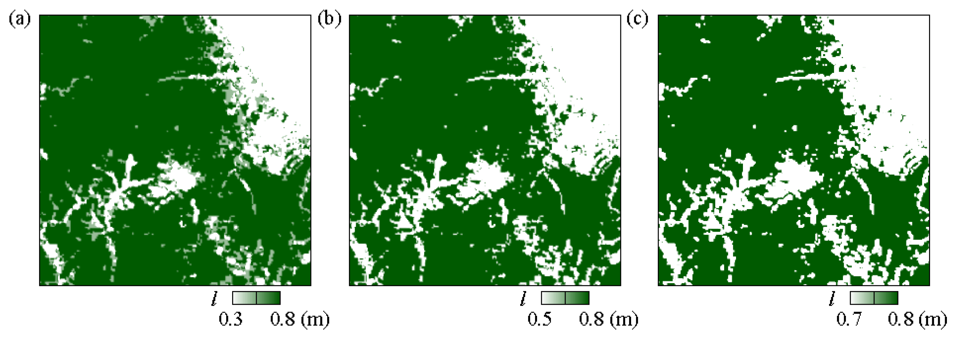
The forest model is triggered when the surface roughness of the corresponding area exceeds a certain reference length (l₀) for activating the forest model. The effect of this reference length on the simulation outcome is studied by conducting simulations with l₀ set to 0.1 m, 0.3 m, and 0.5 m, respectively (as demonstrated in Section 4.3). Figure 6 illustrates the areas of activation for each l₀ value, indicating that the regions where the model is activated shrink as l₀ increases.

The convergence rate is calculated based on the root-mean-square (RMS) values. The equation for the convergence rate is as follows:

$$CR \left(\%\right)=(1-\frac{RMS\left(i\right)}{RMS\left(1\right)})/C\times {10}^4$$

(7)

where CR is the convergence rate, RMS(i) is the residuals of RMS at the iteration of i, and C is the constant value set to 99.5 in the present simulation. The minimum threshold for the convergence rate is 95%, and the maximum number of iterations for the CFD simulation is 25.

The wind speed factor within the computational domain is derived from the CFD simulation, and this value is then used in the process of synthesizing NWP-CFD. This wind speed factor represents the ratio between the actual speed and the speed at an altitude of 10 m in a wide, flat area.

2.5. NWP-CFD Synthesis and Annual Energy Production

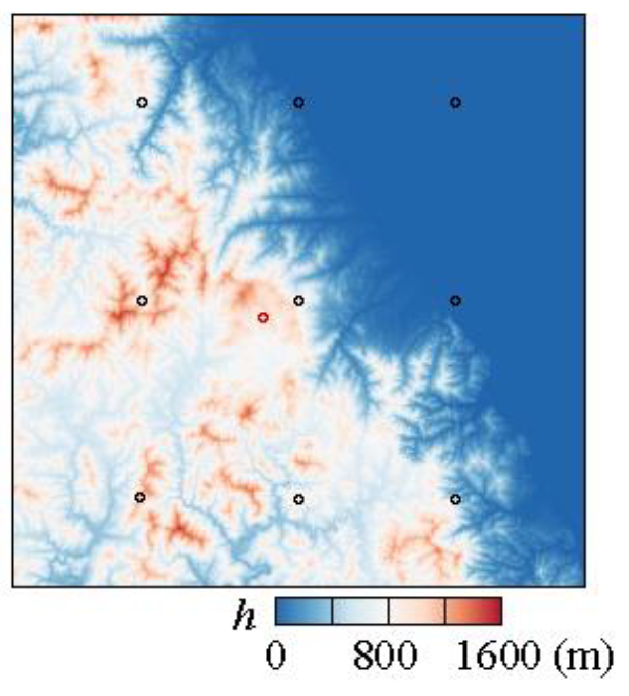
In the CFD procedure outlined in Section 2.4, simulations are conducted in a 3-dimensional computational domain. This results in directional wind speed-up factors at various heights. The synthesis with NWP data is then performed at the height of our interest, specifically 80 m, thereby producing a 2-dimensional wind resource map. The circular symbols in Figure 4a represent the locations of the nine NWP data points utilized in the synthesis process. Each meteorological data point is located at intervals of 20 km.

We use the wind speed data at the height of 320 m to avoid the effects of complex geographical topography on the data. Kim et al. [12] also suggested that the wind speed at 320 m could be appropriate for applying wind speed data that are not distorted by topological effects. On the other hand, for wind speed, there are wind shear effects due to the Coriolis effect, which changes the wind direction with height. Thus, we use the wind direction data at the height of 80 m, similar to that suggested in the previous study [12].

The Weibull scale and shape factors A and k, visualized in Figure 7a,b, with a spatial resolution of 100 m, are derived by integrating the NWP-based meteorological data with the wind speed factor obtained from the CFD simulation [12,15]. From the dataset, it is possible to find those parameters numerically by using optimization algorithms. According to [16], there are three methods of estimating the parameters of the Weibull wind speed distribution: the maximum likelihood method, modified maximum likelihood method, and graphical method. In the present simulation, the maximum likelihood method for the element points is adopted to produce the Weibull parameters as below:

$$k={\left(\frac{{\sum }_{i=1}^n{V}_i^k\ln \left(V_i\right)}{{\sum }_{i=1}^n{V}_i^k}-\frac{{\sum }_{i=1}^n\ln \left(V_i\right)}{n}\right)}^{-1},$$

(8)

$$A={\left(\frac{1}{n}{\sum }_{i=1}^n{V}_i^k\right)}^{\frac{1}{k}},$$

(9)

where n is the number of observations and V_i is the wind speed measured at the interval i [17]. The annual average wind speed and the annual wind speed probability density function are determined by these Weibull coefficients A and k [16].

$$F\left(V\right)=\frac{k}{A}{\left(\frac{V}{A}\right)}^{k-1}\mathrm{e}\mathrm{x}\mathrm{p}\left[-{\left(\frac{V}{A}\right)}^k\right],$$

(10)

$$V_{avg}=A\cdot \Gamma \left(1+\frac{1}{k}\right),$$

(11)

where the velocity is defined as V(m/s), and F(V) is the probability when the wind speed is V during the year. V_avg means the annual average wind speed, and Г() is the gamma function. The annual energy production is derived using the annual wind speed probability density function and the performance curve P(V) of the 3.45 MW turbine [18], and AEP is calculated at 0.5 m/s intervals for wind speeds ranging from 0 to 25 m/s. Figure 8 visualizes the annual average wind speed and annual energy production obtained from the computational domain.

$$AEP=\sum P\left(V\right)\times F\left(V\right)\times 24\times 365,$$

(12)

3. Results of the Convergence Test

3.1. Grid Resolution (Δz_min) Convergence Test

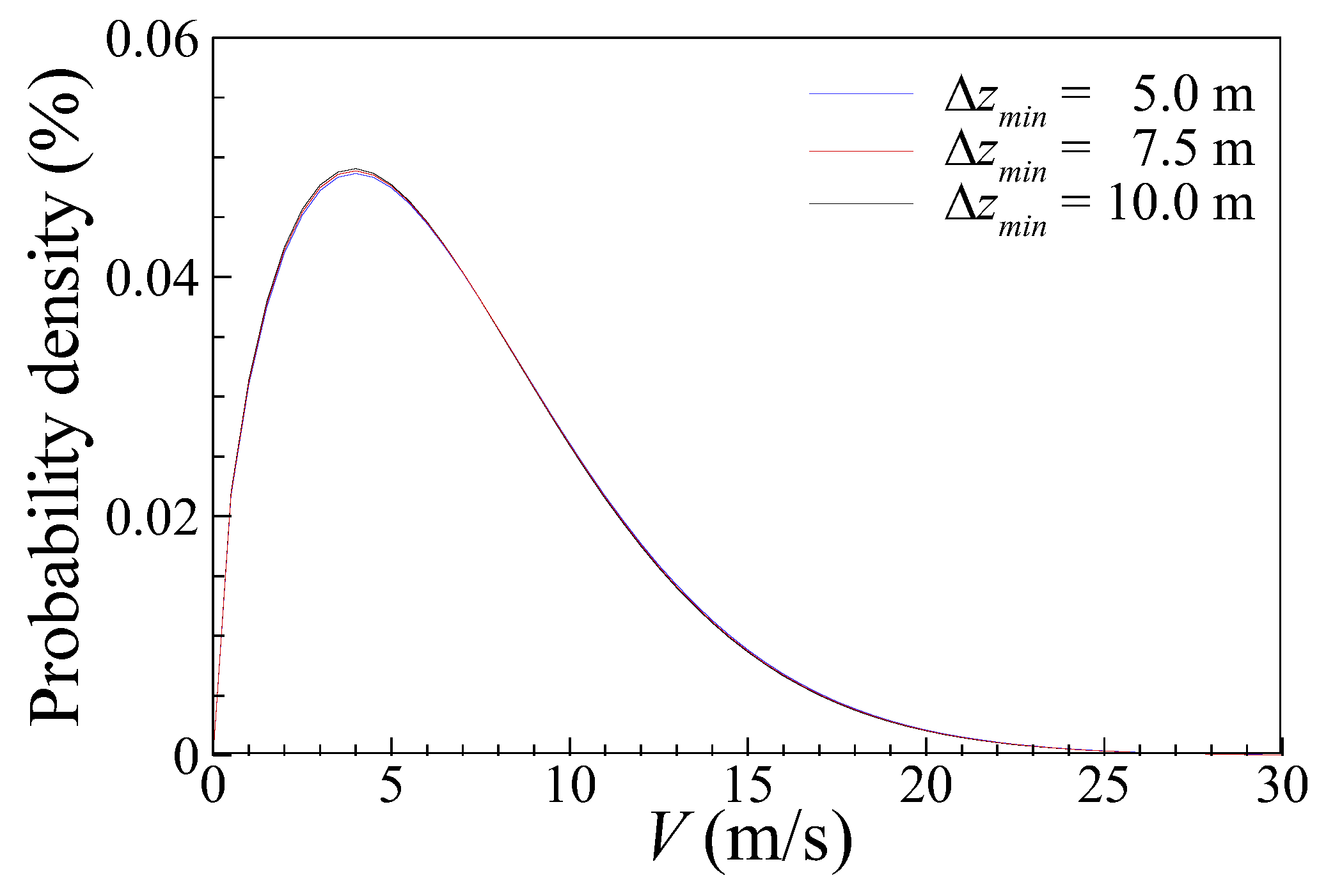
Figure 9 presents wind speed maps for each value of Δz_min, while Figure 10 depicts the wind speed probability density function extracted from the central area (measurement region) of the computational domain. As Δz_min decreases, there is a subtle increase observed in the annual average wind speed and the AEP, with differences in each case being less than 1.5%. In order to reduce computational expenses, the CFD process utilizes a non-uniform grid for the vertical grid, where the size of the grid enlarges with increasing distance from the ground. Δz_min determines the grid size in the vertical direction. A smaller Δz_min allows for a more accurate representation of the velocity distribution close to the ground. Quantitative and qualitative comparisons of the effects of Δz_min, as shown in

Table 1. Annual average wind speed and annual energy production for different minimum vertical grid sizes (Δz_min) obtained using the NWP-CFD method at the measuring points shown in Figure 9.

Δzmin (m)	Vavg (m/s)	AEP (MW)
5	6.959	10,572.829
7.5	6.928	10,504.428
10	6.902	10,446.890

and Figure 10, reveal that the impact of Δz_min is minimal within a range of 10 m. This suggests that a Δz_min of 10 m is a suitable setting from a computational cost perspective.

3.2. Convergence Test of the Wind Direction Resolution (Δdir)

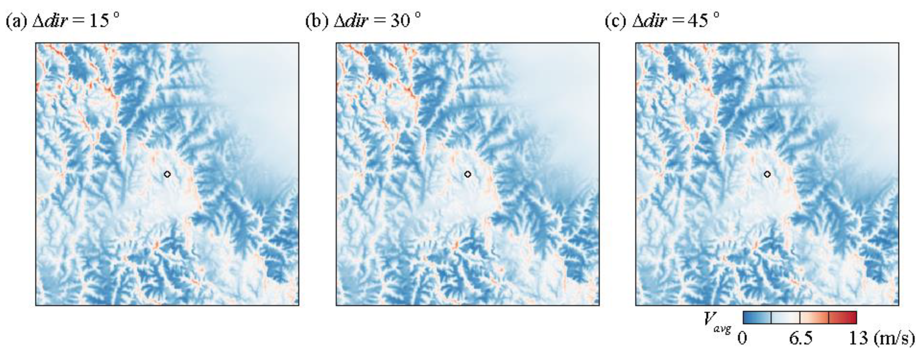
Figure 11 presents the wind speed maps generated by adjusting Δdir for each direction. As Δdir decreases, both the annual average wind speed and AEP tend to reduce. Figure 12 demonstrates the probability density function of the wind speed derived from the central zone (measurement area) of the computational domain. According to

Table 2. Annual average wind speed and annual energy production for different Δdir obtained by the NWP-CFD method at the position which is denoted by the circular symbol in Figure 10.

Δdir (o)	Vavg (m/s)	AEP (MW)
15	6.889	10,423.650
30	6.902	10,446.890
45	6.976	10,597.309

, when Δdir is set at 45°, there is approximately a 1.6% discrepancy in AEP compared to when Δdir is set at 30°. However, the difference in AEP between Δdir at 30° and 15° is less than 0.3%, showing that the impact of Δdir on the simulation result is negligible within the 30° range. This finding suggests that setting Δdir to 30° is adequate when considering the computational cost.

3.3. Influence of l₀ Regularization on Computational Result

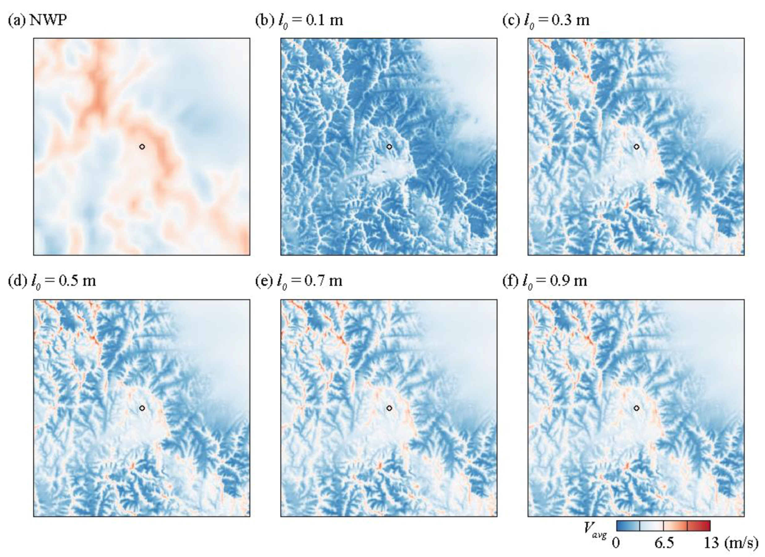
As depicted in Figure 13 and

Table 3. Annual average wind speed and annual energy production for each method and l₀ at the position which is presented by the circular symbol in Figure 13.

l0 (m)	Vavg (m/s)	AEP (MW)
0.1	5.188	6041.079
0.2	6.302	9056.832
0.3	6.696	10,000.072
0.4	6.833	10,298.702
0.5	6.902	10,446.890
0.6	6.988	10,630.660
0.7	7.082	10,826.366
0.8	7.063	10,787.763
0.9	7.039	10,738.914

, as the parameter l₀ decreases, the forest model is activated over a broader area, which in turn results in a decline in both the annual average wind speed and annual energy production (AEP). The wind speeds calculated for each value of l₀ are visualized in Figure 13. Contrasting Δz_min and Δdir, where the differences between the wind speed map and the probability density function are minimal, a substantial difference can be observed with varying l₀.

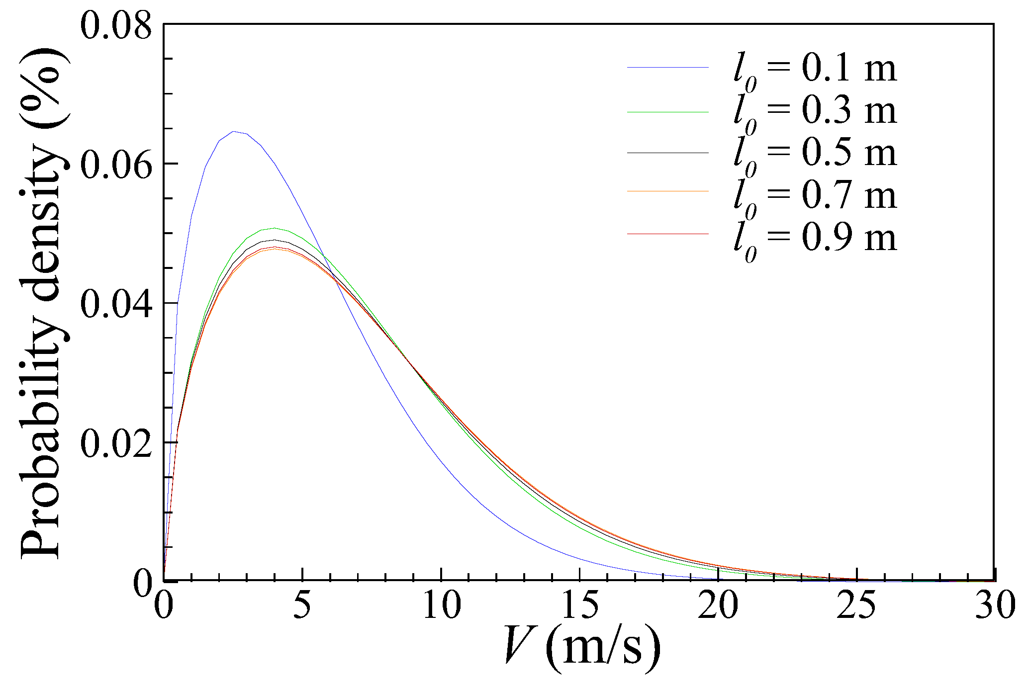
Figure 14 presents the annual wind speed probability distributions for each method and l₀ value in the measurement region. It is apparent that the probability density function is affected by the value of l₀ changes. As such, meticulous calibration of l₀ appears to be crucial to ensure the accuracy of wind speed predictions and the corresponding annual energy production (AEP) estimates. The underestimation of wind speed, particularly in regions with high wind speeds, when l₀ is set to 0.1 m, suggests that the forest model may be too active in these areas, thereby affecting the simulation’s capacity to represent the wind dynamics in these regions accurately. Conversely, when l₀ is set to 0.2 m or higher, the forest model is activated across a narrower area. This emphasizes the influence of surface roughness, as represented by l₀, on the wind distribution and, consequently, on the performance of the wind resource prediction. When l₀ is higher than 0.3, the probability density function shows reduced sensitivity to the activation length.

4. Quantitative Evaluation Using the NWP-MCP-CFD Method

4.1. Measured Meteorological Data

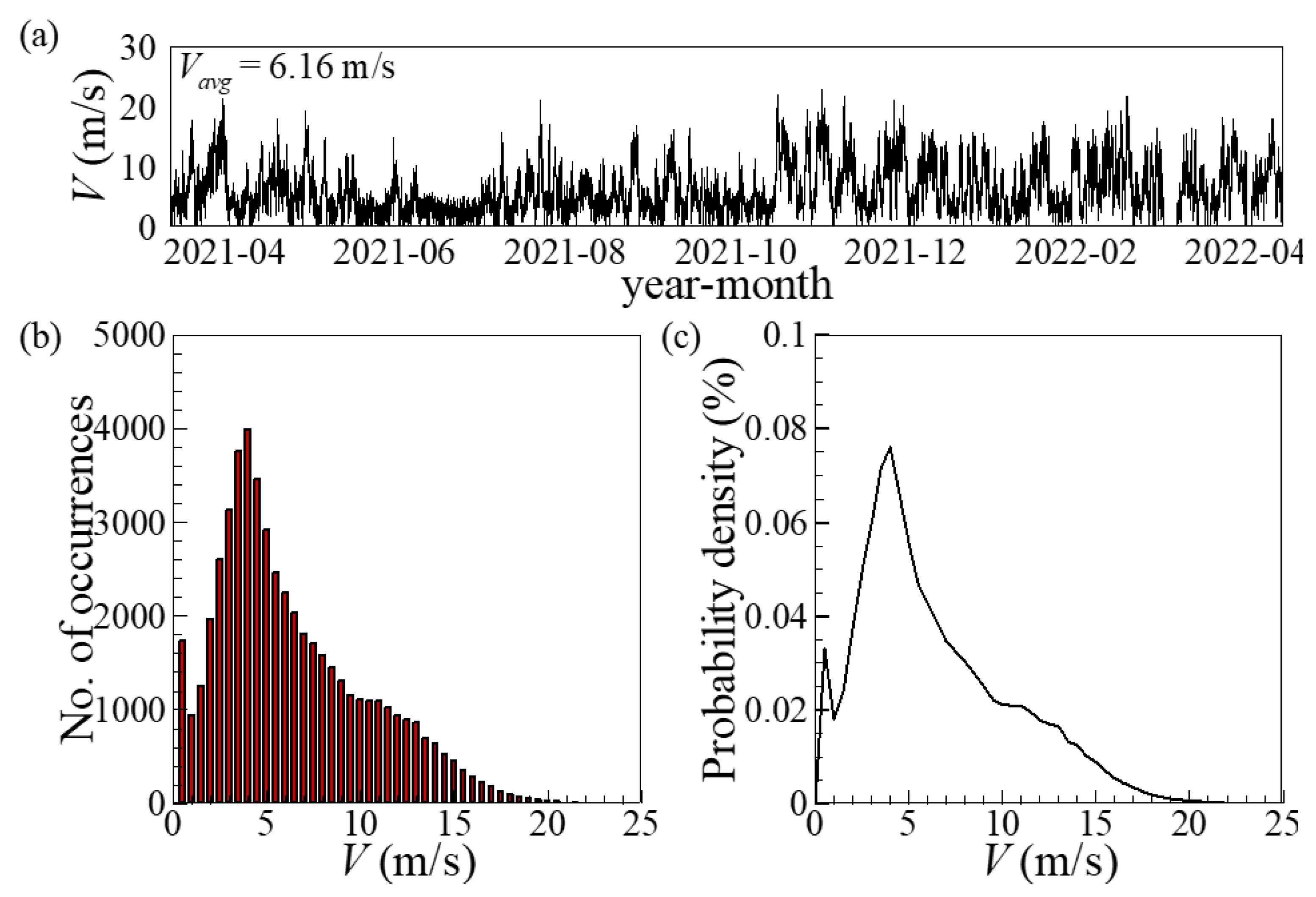
Meteorological data for quantitative evaluation were measured in Pyeongchang, Gangwon, in 2021 (latitude—27.73, longitude—128.67). The wind velocity measurement altitude is 80 m, and the temporal resolution is 10 min. Figure 15 shows the annual wind speed distribution and density function of the measured data, showing an average wind speed of 6.16 m/s, corresponding to the annual energy production (AEP) of 9344 MW.

4.2. ERA5 Meteorological Data

To compare the meteorological data based on the NWP method produced in 2010 with the observational data acquired in 2021, we employ the measure correlate predict (MCP) method. The MCP method is utilized to adjust short-term meteorological data to long-term meteorological data [19,20], and a detailed explanation of this method can be found in Section 4.3. The long-term meteorological data used in the MCP method are ERA5 produced by the European Center for Medium-Range Weather Forecasts (ECMWF), which have a higher resolution compared to the existing reanalysis data [21,22,23]. Figure 16 visualizes the wind speed at an altitude of 100 m of the ERA5 data of the location (black dot located at the center of Figure 17, latitude—37.75, longitude—128.75) closest to the measurement location (red dot in Figure 16), and its temporal resolution is 1 h.

4.3. Measure Correlate Predict (MCP) Method

For the correction of short-term meteorological data, long-term reanalysis data collected near the measurement location are employed. The relationship between these two datasets is analyzed, as depicted in Figure 18a, to predict the meteorological conditions beyond the measurement timeframe, as shown in Figure 18b. Figure 18c displays a magnified view of the dashed red box region (denoted by A) in Figure 17, presenting the reconstructed NWP data based on ERA5 data, corresponding to the same temporal frame as the measured data in 2021. We incorporate the reconstructed NWP data (NWP-MCP data) into the CFD simulation (NWP-MCP-CFD) and conduct a quantitative evaluation of l0 by comparing it with the measured data. To produce NWP-MCP data, the four MCP methods are used in the present study by utilizing the Windographer v4.2.21 software.

Linear Least Squares (LLS), Total Least Squares (TLS), Variance Ratio (VR), and Matrix Time Series (MTS).

The LLS algorithm associates short-term data with long-term data using a linear least squares process. This algorithm aims to find a linear relationship equation that minimizes the sum of squared errors between the two datasets. The linear relationship equation is determined within the range shown in Figure 18a, and based on that equation, the short-term data are calibrated.

The TLS algorithm, also known as orthogonal least squares, is similar to the LLS algorithm in that it finds a linear equation that minimizes the sum of squared errors. However, the key difference lies in how the error is defined. In the LLS algorithm, the error is defined as the vertical distance between each point and the linear equation. In contrast, the TLS algorithm defines the error as the shortest distance between variables and the linear equation.

The VR algorithm is designed to represent the relationship between two datasets using a linear model in the form of y = ax + b [24]. The algorithm determines the parameters of the linear model by setting them in such a way that the variance of the predicted data matches the variance of the short-term meteorological data.

The MTS algorithm, an enhanced form of the traditional Matrix method, forecasts weather by acknowledging the random nature of the relationship between two datasets [25]. The meteorological predictions obtained from the MTS method provide a more accurate depiction of the meteorological distribution compared to those derived from the linear MCP algorithm. According to a comparison study by Hyun et al. [26] on data from four Korean locations, the Matrix method generated estimates that closely resembled actual measurements.

Figure 19 presents the wind speed probability density function derived from conducting an NWP-MCP analysis using the four methods mentioned above. The measured data are indicated by a circular symbol. The MTS method, represented by the blue line, appears to closely follow the trend of the measured data in the wind speed range of 0–13 m/s, but it diverges from this trend at higher speeds. Conversely, the LLS method, shown in green, deviates somewhat from the measured data in the low-speed region yet aligns more accurately at speeds above approximately 12 m/s. In comparison, the other three methods exhibit relatively poor performance in predicting the actual measured data at speeds over 12 m/s, particularly when compared to the LLS method. However, as noted earlier, since the effects of geographic characteristics such as land elevation and surface roughness are not considered in the wind data produced using NWP or NWP-MCP, the predictive performance cannot be solely judged based on the results depicted in Figure 19. Therefore, to better predict the measured data, the coupled NWP-MCP-CFD method is employed, taking into account these geographical characteristics.

4.4. Quantitative Evaluation of NWP-MCP-CFD Coupled Method

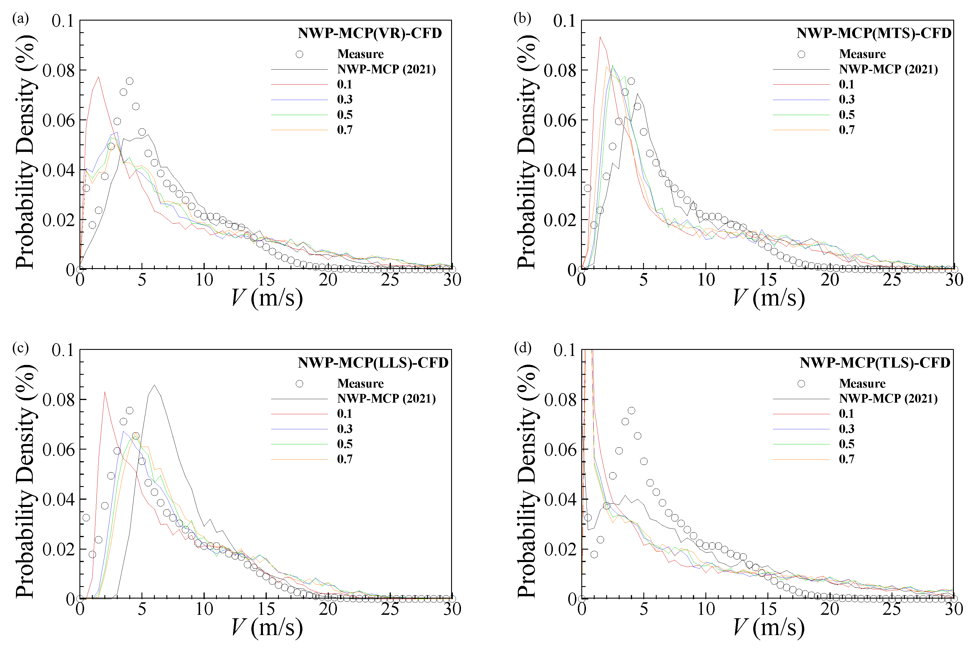
Figure 20 displays the wind speed probability density function obtained using the NWP-MCP-CFD method for different l₀ values, aiming to evaluate their performance by comparing them with the actual measured data (indicated by a circular symbol). Figure 20a–d present the results of employing the four different MCP methods. The NWP-MCP data are represented by the black solid line, while the NWP-MCP-CFD results with different l₀ values are depicted by colored lines. After integrating NWP-MCP data into the CFD simulation, the wind speed exhibits a generally decreasing trend, accounting for surface elevation and its roughness. Consequently, the probability density function slightly shifts to the left in Figure 20. Qualitatively comparing these results to the measured data, the VR and TLS methods demonstrate poorer performance compared to the MTS and LLS methods. The NWP-MCP data using the MTS method, in particular, show a trend similar to the measured data around the wind speed region of ~12 m/s, as seen in Figure 19. However, this trend diverges from the measured data after being incorporated into the CFD simulation in Figure 20b due to the consideration of geographical characteristics. On the other hand, the CFD simulation using the NWP-MCP data from the LLS method shows relatively good agreement across a wide range of wind speeds in Figure 20c. When l₀ is 0.1 (denoted by the red line), the predicted probability density distribution deviates from the measured data in the wind speed range of approximately 3 m/s to 10 m/s, with a corresponding R² value of about 0.76 in

Table 4. R-square values of the results from the NWP-MCP-CFD method as compared to the real measured data in 2021.

MCP Method	${\mathit{l}}_0$	VR	MTS	LLS	TLS
R2 (NWP-MCP-CFD)	0.1	0.512012191	0.478613892	0.764439075	0.172561868
	0.3	0.807865206	0.700670966	0.872962351	0.215983043
	0.5	0.848751756	0.734510185	0.818943799	0.220863726
	0.7	0.869351275	0.632518286	0.771429777	0.219811708

. As the activation length l₀ increases to 0.3, the distribution shifts to the right, and the optimal R² value reaches approximately 0.87. The NWP-MCP method, when using the LLS approach, deviates from the measured data in the low wind speed region of approximately 0 to 12 m/s, as discussed in Figure 19. However, it demonstrates optimal estimation performance after being incorporated into the CFD simulation, taking into account geographical characteristics. Here, the R² value corresponds to 0.87 at an activation length of 0.3. This implies that the LLS method effectively reconstructs NWP data for a specific period, making it suitable for application in the NWP-MCP-CFD coupled method.

Table 5. Computational time for the CFD simulation and the synthesis procedures using the Intel^®® Xeon^®® E5-2687W.

Simulation	${\mathit{l}}_0$	CFD	Synthesis
Computational Time	0.1	181 h 30 min	89 h 30 min
	0.3	154 h 57 min	91 h 24 min
	0.5	181 h 5 min	89 h 24 min
	0.7	188 h 57 min	97 h 21 min

shows the computational time for the CFD simulation and the synthesis procedures using the Intel^®® Xeon^®® E5-2687W. The averaged computational time for the CFD and synthesis procedures are about 176 h and 92 h, respectively.

5. Conclusions

This study presents a comprehensive comparison and analysis of KIER-WindMap data, NWP-CFD data, and corrected measurement data. Additionally, it provides an optimization of input parameters for the NWP-CFD method, an aspect that was underexplored in previous research. The study has culminated in several crucial conclusions:

• Our simulations, informed by parameters obtained from previous studies, show an approximate 8.5% deviation from the corrected measurement data. This suggests that although the NWP-CFD approach is more reliable for wind resource predictions in complex terrains like Korea compared to the standalone NWP method, further parameter optimization is necessary to enhance prediction accuracy.
• In the NWP-CFD downscaling method, Δz_min, Δdir, and l₀ emerge as three key influencing factors. Our analysis suggests that the effects of Δz_min and Δdir on the simulation outcomes are relatively minimal once their values reach a stabilized region. Thus, within this optimal range, changes in Δz_min and Δdir do not significantly impact the simulation results.
• On the other hand, the l₀ factor exerts a significant influence on the forest model activation area and the ensuing simulation results. Adjusting l₀ according to the specific land characteristics is found to be essential for more accurate wind resource prediction, emphasizing the importance of fine-tuning model parameters based on local conditions. The sensitivity of the wind distribution to the activation length decreases when the activation length exceeds 0.3.
• The meteorological data, derived from applying the NWP-MCP using the MST method, demonstrate good estimation performance compared to the measured data before considering geographical characteristics. Upon incorporating these data into the CFD simulation, the highest R2 value, approximately 0.87, is observed in the NWP-MCP (LLS)-NWP method. This suggests that the LLS method could be an effective option for projecting short-term NWP data onto long-term meteorological data prior to employing the NWP-MCP-CFD coupled method.

The insights derived from this study underscore the importance of thoughtful parameter selection and refinement in wind resource prediction models. Further work should focus on the development and application of robust methodologies for parameter adjustment in specific local conditions, thus enhancing the precision of wind resource predictions.

References

1. Zou, C.; Zhao, Q.; Zhang, G.; Xiong, B. Energy revolution: From a fossil energy era to a new energy era. Nat. Gas Ind. B 2016, 3, 1–11. [Google Scholar] [CrossRef]
2. BP. BP Statistical Review of World Energy; BP: London, UK, 2015; Available online: http://large.stanford.edu/courses/2015/ph240/zerkalov2/docs/bp2015.pdf (accessed on 1 June 2023).
3. Sadorsky, P. Wind energy for sustainable development: Driving factors and future outlook. J. Clean. Prod. 2021, 289, 125779. [Google Scholar] [CrossRef]
4. BP. BP Statistical Review of World Energy; BP: London, UK, 2019; Available online: https://www.bp.com/content/dam/bp/business-sites/en/global/corporate/pdfs/energy-economics/statistical-review/bp-stats-review-2019-full-report.pdf (accessed on 1 June 2023).
5. Kim, C.S. New & Renewable Energy Statistics 2020, 2021st ed.; Korea Energy Agency: Ulsan, Republic of Korea, 2021. [Google Scholar]
6. Shikha, S.; Bhatti, T.; Kothari, D. A review of wind-resource-assessment technology. J. Energy Eng. 2006, 132, 8–14. [Google Scholar]
7. Gharaati, M.; Xiao, S.; Wei, N.; Martinez-Tossas, L.A.; Dabiri, J.O.; Yang, D. Large-eddy simulation of helical- and straight-bladed vertical-axis wind turbines in boundary layer turbulence. J. Renew. Sustain. Energy 2022, 14, 053301. [Google Scholar] [CrossRef]
8. Al-Yahyai, S.; Charabi, Y.; Gastli, A. Review of the use of numerical weather prediction (NWP) models for wind energy assessment. Renew. Sustain. Energy Rev. 2010, 14, 3192–3198. [Google Scholar] [CrossRef]
9. Done, J.; Davis, C.A.; Weisman, M. The next generation of NWP: Explicit forecasts of convection using the Weather Research and Forecasting (WRF) model. Atmos. Sci. Lett. 2004, 5, 110–117. [Google Scholar] [CrossRef]
10. Bang, C.H.; Lee, J.W.; Hong, S.Y. Predictability experiments of fog and visibility in local airports over Korea using the WRF model. J. Korean Soc. Atmos. Environ. 2008, 24, 92–101. [Google Scholar]
11. Byun, U.Y.; Hong, S.Y.; Shin, H.; Lee, J.W.; Song, J.I.; Hahm, S.J.; Kim, J.K.; Kim, H.W.; Kim, J.S. WRF-based short-range forecast system of the Korea Air Force: Verification of prediction skill in 2009 summer. Atmosphere 2011, 21, 197–208. [Google Scholar]
12. Kim, H.G.; Lee, H.W. Wind Resource Assessment of Baekado by NWP-CFD Downscaling. Korean Soc. New Renew. Energy 2019, 15, 117. [Google Scholar]
13. Che, Y.; Salazar, A.A.; Peng, S.; Zheng, J.; Chen, Y.; Yuan, L. A multi-scale model for day-ahead wind speed forecasting: A case study of the Houhoku wind farm, Japan. Sustain. Energy Technol. Assess. 2022, 52, 101995. [Google Scholar] [CrossRef]
14. Durán, P.; Cathérine, M.; Pau, C. A new meso-microscale coupled modelling framework for wind resource assessment: A validation study. Renew. Energy 2020, 160, 538–554. [Google Scholar] [CrossRef]
15. Kim, J.; Hwang, S.J.; Kim, J.Y.; Park, S.G.; Kim, H.G. High-Resolution Mapping of Onshore Wind Resource Using NWP-CFD Downscaling. J. Wind Eng. Inst. Korea 2022, 26, 3–8. [Google Scholar] [CrossRef]
16. Seguro, J.V.; Lambert, T.W. Modern estimation of the parameters of the Weibull wind speed distribution for wind energy analysis. J. Wind Eng. Ind. Aerodyn. 2000, 85, 75–84. [Google Scholar] [CrossRef]
17. Paulo, A.C.R.; Ricardo, C.S.; Carla, F.A.; Maria, E.V.S. Comparison of seven numerical methods for determining Weibull parameters for wind energy generation in the northeast region of Brazil. Appl. Energy 2012, 89, 395–400. [Google Scholar]
18. Kim, M.J.; Song, Y.; Peak, I. Development of an In-house Code to Predict Annual Energy Production and Economic Analysis of Wind Farms Using CFD Results. J. Wind Energy 2020, 11, 23–30. [Google Scholar]
19. Polo, J.; Wilbert, S.; Ruiz-Arias, J.A.; Meyer, R.; Gueymard, C.; Suri, M.; Martin, L.; Mieslinger, T.; Blanc, P.; Grant, I.; et al. Preliminary survey on site-adaptation techniques for satellite-derived and reanalysis solar radiation datasets. Sol. Energy 2016, 132, 25–37. [Google Scholar] [CrossRef]
20. Carta, J.A.; Velázquez, S.; Cabrera, P. A review of measure-correlate-predict (MCP) methods used to estimate long-term wind characteristics at a target site. Renew. Sustain. Energy Rev. 2013, 27, 362–400. [Google Scholar] [CrossRef]
21. Hersbach, H.; Bell, B.; Berrisford, P.; Hirahara, S.; Horányi, A.; Muñoz-Sabater, J.; Nicolas, J.; Peubey, C.; Radu, R.; Schepers, D.; et al. The ERA5 global reanalysis. Q. J. R. Meteorol. Soc. 2020, 146, 1999–2049. [Google Scholar] [CrossRef]
22. Kim, J.Y.; Hwang, S.J.; Kim, H.G.; Park, C.Y.; Jeong, J.Y. Site Adaptation of the Reanalysis Data ERA5 on the Power Prediction of Wind Farms. J. Korean Sol. Energy Soc. 2022, 42, 79–91. [Google Scholar] [CrossRef]
23. Gualtieri, G. Reliability of era5 reanalysis data for wind resource assessment: A comparison against tall towers. Energies 2021, 14, 4169. [Google Scholar] [CrossRef]
24. Rogers, A.L.; Rogers, J.W.; Manwell, J.F. Comparison of the performance of four measure–correlate–predict algorithms. J. Wind Eng. Ind. Aerodyn. 2005, 93, 243–264. [Google Scholar] [CrossRef]
25. Lambert, T.; Grue, A. The matrix time series method for MCP. In Proceedings of the WINDPOWER 2012 Conference, Atlanta, GA, USA, 3–6 June 2012. [Google Scholar]
26. Hyun, S.G.; Jang, M.S.; Ko, S.H. Variability Characteristics Analysis of the Long-term Wind and Wind Energy Using the MCP Method. J. Korean Sol. Energy Soc. 2013, 33, 1–8. [Google Scholar] [CrossRef]
Figure 1. Flowchart of the NWP-CFD coupled method to downscale mesoscale wind data. (a) Directional CFD simulation by using a DEM and SRTM data. (b) Results of directional wind speed-up factor by performing the CFD simulation. (c) Mesoscale data obtained from WRF simulation. (d) Synthesis results (Weibull coefficients A and k) by combining the directional wind speed-up factor with the mesoscale wind data. (e) Wind turbine power curve. (f) Annual energy production based on the synthesis results and the turbine power curve.
Energies 17 00648 g001
Figure 2. (a) Time history of annual wind speed, (b) annual wind speed distribution, and (c) annual wind speed probability density function based on the meteorological data by NWP method in 2010. The coordinates of the location under study are (37.73, 128.69) for latitude and longitude, respectively.
Energies 17 00648 g002
Figure 3. The computational domain, represented by a red box measuring 50 km × 50 km, is centered around the measurement area used for CFD simulation in the UTM zone 52 n coordinates.
Energies 17 00648 g003
Figure 4. For the CFD simulation, two data sources are used: (a) digital elevation model (DEM)—these are the Shuttle Radar Topography Mission (SRTM) data created by the National Geographic Information Institute, offering a resolution of 90 m; (b) surface roughness—these data come from the land cover dataset provided by the Ministry of Environment of Korea. The NWP data are used at the positions denoted by the circular symbols in (a).
Energies 17 00648 g004
Figure 5. (a) Horizontal grid generation for the CFD simulation. The grids are denoted by thin black solid line. The thick black dashed line and the red solid line correspond to those in Figure 3. The horizontal grid resolution inside the red solid line is 100 m. (b) Magnified view of (a) in the region denoted by blue dashed line.
Energies 17 00648 g005
Figure 6. Visualization of the activation area according to the forest model activation reference length (l0). (a) l0 = 0.3 m, (b) l0 = 0.5 m, and (c) l0 = 0.7 m.
Energies 17 00648 g006
Figure 7. (a) Weibull coefficient A and (b) Weibull coefficient k as a result of NWP-CFD synthesis process.
Energies 17 00648 g007
Figure 8. (a) Annual average wind speed and (b) annual energy production for Δzmin = 10.0 m, Δdir = 30°, l0 = 0.5 m.
Energies 17 00648 g008
Figure 9. Annual average wind speed map derived from NWP-CFD method at (a) Δzmin = 5.0 m; (b) Δzmin = 7.5 m; (c) Δzmin = 10.0 m. The data obtained by the NWP-CFD coupled method at the position denoted by the circular symbol are compared with the real measurement data in Section 4.4.
Energies 17 00648 g009
Figure 10. The wind speed probability density function, computed for each value of Δzmin at the position denoted by the circular symbol in Figure 8.
Energies 17 00648 g010
Figure 11. Annual average wind speed map derived from NWP-CFD method at (a) Δdir = 15°; (b) Δdir = 30°; (c) Δdir = 45°. The data obtained by the NWP-CFD coupled method at the position denoted by the circular symbol are compared with the real measurement data in Section 4.4.
Energies 17 00648 g011
Figure 12. Wind speed probability density function derived by calculating each Δdir at the position which is denoted by the circular symbol in Figure 10.
Energies 17 00648 g012
Figure 13. Annual average wind speed map derived from (a) NWP method and (bf) NWP-CFD method. The reference length for activating the forest model is given by (b) l0 = 0.1 m; (c) l0 = 0.3 m; (d) l0 = 0.5 m; (e) l0 = 0.7 m; (f) l0 = 0.9 m. The data obtained by the NWP-CFD coupled method at the position denoted by the circular symbol are compared with the real measurement data in Section 4.4.
Energies 17 00648 g013
Figure 14. Wind speed probability density function derived by calculation of each method and l0 at the measuring points shown in Figure 13.
Energies 17 00648 g014
Figure 15. (a) Time history of annual wind speed, (b) annual wind speed distribution, and (c) annual wind speed probability density function based on the meteorological data measured in the Pyeongchang region of Gangwon-do in 2021. The coordinates of the location under study are (37.7299, 128.6724) for latitude and longitude, respectively.
Energies 17 00648 g015
Figure 16. Time history of annual wind speed from 1979 to 2022 on ERA5 meteorological data. The coordinates of the location under study are (37.7500, 128.7500) for latitude and longitude, respectively.
Energies 17 00648 g016
Figure 17. Locations of meteorological data. The locations of ERA5 and NWP-based meteorological data used for strategic evaluation are indicated by black circular symbols, while the locations of actual measured data are represented by red circular symbol.
Energies 17 00648 g017
Figure 18. (a) Relationship between annual wind speed time series data of NWP meteorological data (black line) and ERA5 meteorological data (red line); (b) annual wind speed time series data of meteorological data derived by MCP method based on the correlation between the two meteorological data (blue line). Box A is clearly shown in (c).
Energies 17 00648 g018
Figure 19. Wind speed probability density function derived by conducting an NWP-MCP using the four MCP methods. The measured data are located at the position denoted by the red dot, while NWP-MCP data are at the center of the black dots in Figure 17.
Energies 17 00648 g019
Figure 20. Wind speed probability density function obtained from the measured data and the NWP-MCP-CFD methods for different activation lengths of the forest model l0. The MCP methods are (a) VR, (b) MTS, (c) LLS, and (d) TLS.
Energies 17 00648 g020