Key Performance Indicators for Decision Support in Building Retrofit Planning: An Italian Case Study

Abstract

To achieve climate and energy goals in the building sector, the current pace of renovating existing structures must double, overcoming prevailing barriers. Key Performance Indicators play a pivotal role in science-based decision making, emphasizing both direct and indirect benefits of building retrofits. The authors aim to contribute to proper metric identification for multi-perspective building performance assessment and formulate a methodology supporting energy planning decisions. They introduce the Global Cost per Emission Savings (GCES), an aggregated indicator encompassing both public (CO₂ emissions) and private (global cost) perspectives of diverse retrofit technologies for building HVAC systems. Applied to the Italian residential building stock via the Reference Building approach, the methodology is tested using condensing gas boilers, biomass boilers, and electric heat pumps, revealing diverse environmental and economic performances. Addressing the establishment of effective decision-support tools for policymakers, the paper explores the potential impact of various policies on the favorability of technologies. Different policy scenarios are delineated to analyze how distinct approaches may influence the attractiveness of technologies. Notably, in the baseline scenario, biomass boilers hold an advantage over heat pumps according to the GCES index. However, scenarios involving technology-specific incentives or a greenhouse gases emission tax failed to alter the technological ranking, leaving heat pumps financially uncompetitive. In contrast, the TXPM scenario positions heat pumps as the most financially appealing option, penalizing biomass boilers for high particulate matter emissions.

1. Introduction

To boost the energy transition process and move towards a climate-neutral European Union (EU), mid-term (2030) and long-term (2050) objectives were set at the European level. Mid-term goals up to 2030, regulated by the “Fit for 55” package, include a 55% cut in greenhouse gas (GHG) emissions, compared to the 1990 levels, and a 40% share of renewable energy in the EU energy mix [1]. Within this context, the role of the building sector is widely recognized, due to its energy and environmental impacts, and its untapped potential for savings has been emphasized in different studies [2,3]. Not by chance, the European Roadmap to 2050 places significant emphasis on this sector, aiming for a 90% reduction in emissions by 2050 compared to the 1990 levels [4]. Achieving this ambitious goal requires a substantial acceleration of the renovation process [5], as focusing solely on new buildings would be overly simplistic and inadequate, particularly in the European context. The European Commission has estimated that, at the current rates of construction and demolition, approximately 70% of the buildings that will be in use in 2050 are already standing [2], and 75% of the European building stock is currently energy inefficient [6], highlighting that renovation will represent a key challenge in the following decades.

From this background, it emerges how the energy transition of the building sector is asking for an unprecedented effort to policymakers, stakeholders, and individuals, and must be accompanied by approaches that are able to support them in making rational decisions. In this framework, the use of Key Performance Indicators (KPIs) is particularly common, being identified as the most suitable approach for combining “energy efficiency improvement and policy evaluation [7]”. KPIs are effectively used for assessing building performances, as well as for supporting the development of energy policies for driving the sector, using them as decision-making tools [8]. Indeed, their definition allows us to set and monitor medium- and long-term objectives, as well as to translate measured data into “usable knowledge”, to be easily understandable by different users and also non-experts, in the different stages of the life of a building.

In the literature, renovation projects and strategies are commonly evaluated with a multi-dimensional standpoint. According to Kylili et al. [9], prior research commonly organizes KPIs into eight overarching categories, further subdivided into specific sub-categories. These classes encompass economic, environmental, social, technological, time-related, quality-related, disputes-related, and project-administration-related KPIs, particularly when assessing the sustainability of a renovation project [9]. Indeed, it is widely recognized that the definition of the most suitable retrofit options for buildings is usually a multi-objective optimization problem [10], where different criteria must be taken into account. They can be financial criteria, quantified whether adopting a life-cycle approach [11,12,13,14,15,16] or not, dealing only with investment costs [17,18]. Various financial indicators are used, including the Life Cycle Cost [11,13], the Net Present Value [12,16], the simple Payback period [14], and the Global Cost [19,20]. Selected KPIs in assessing retrofit options can be energy-related, such as energy consumption [18], building load [17], or energy savings [14,21], or environmentally related, like CO₂eq emissions [13,18] or environmental impacts evaluated via Life Cycle Assessments [22,23]. Finally, other criteria to control can be related to thermal comfort via the maximization of, for example, the Predictive Mean Vote [21] as a metric. In the works just mentioned, the criteria are sometimes considered alone or in combination with other KPIs, adopting a specific standpoint for the evaluation, which is typically one of an investor/decision maker. Indeed, as stressed by Jafari et al. [10], this type of decision maker can affect the selection of objective functions in assessing retrofit options.

Despite the efforts of setting multiple-objective functions in the assessment found in previous studies, the authors believe that a step forward would be the identification of KPIs able to combine conflicting viewpoints. KPIs have to be not only multi-domain but also multi-perspective in order to be used to assess alternative policies. This is particularly relevant in face of the need to keep together contrasting standpoints and to increase awareness about the non-financial benefits related to building renovation, motivating users in adopting more low-carbon retrofit measures. Indeed, it is important for policy discussion to prioritize renovation measures representing the best compromise between costs and benefits, including those going beyond the purely financial convenience [24], which is still the main motivation driving investors’ choices.

To achieve this goal, policymakers should formulate effective policy measures capable of narrowing the persisting gap between “green and profitable investments.” This involves steering the market towards the adoption of low-carbon solutions by appropriately adjusting their costs for consumers to accurately reflect their superior environmental performance [25].

Paper Positioning

In light of the above, this paper wants to contribute to the identification of proper metrics for assessing building performances from multiple perspectives. The newly developed KPIs take into account the varied interests of different stakeholders involved in the renovation process. In the paper, the authors have also introduced a methodology to facilitate decision-making processes within the building sector and to disseminate information about prevalent technological alternatives. To move towards an effective energy planning for the renovation of the building stock, the paper highlights the cruciality of having a picture of the possible alternative technological solutions for building retrofit (focusing on the replacement of thermal generators) with clear information about their performances. Moreover, the authors intend to propose decision-making tools (either graphical or analytical) in support of policymakers, to assess the effect that some policy measures affecting the private sphere (e.g., price mechanisms, environmental taxes, and incentive mechanisms) could have on the reciprocal competitiveness of the technologies under investigation.

The novelty of the proposed indicator lies in its nature as an aggregated metric, enabling the assessment of both economic (private) and environmental (public) perspectives through a single value. It represents the trade-off between these two dimensions, unlike other methods such as multi-criteria analysis, which requires multiple indicators, diverse criteria, and input from experts in different sectors to identify the optimal solution [26]. Through the newly developed metric, the authors’ aim is to combine the two variables (cost and GHG emission) into a unified indicator, deviating from the conventional practice of relying on a single variable [17,18,19,20,21,22,23]. The objective is not to determine the optimal technology but rather to formulate an aggregated indicator that facilitates the comparison of multiple aspects within a single value. This approach aids in comprehending how outcomes may vary when considering two variables, typically with opposing objectives. Consequently, this indicator proves valuable to decision makers, not for the selection of the best technology, but for assessing the relative positioning of multiple technologies. This empowers decision makers to formulate appropriate policies that enhance the competitiveness of one technology over another.

The paper is structured as follows: Section 2 describes the methodology and the evaluation workflow. Then, in Section 3, the methodology is exemplified by its application to the case study of the Italian residential building stock, while Section 4 summarizes the main outcomes. Finally, in Section 5, conclusions about replicability, strengths, and weaknesses of the methodology are provided, together with a description of the challenges related to the specific application and of future developments on the research.

2. Materials and Methods

In this paper, the authors propose a methodological framework to be used as a decision-support tool for decision makers in building energy planning. The methodology here presented is deployed with the scope of comparing a set of alternative technologies for building retrofit from a multi-perspective standpoint, by identifying specific KPIs for assessing their financial and environmental performance trade-offs. Indeed, aiming to combine the possible conflicting interests of private and public stakeholders in case of technological competitiveness, KPIs are used to reflect the conflict between the private benefits arising from the selection of the most financially attractive solutions and the public risks associated to private decisions, in case the most financially convenient solution is at the same time the most environmentally risky. To this purpose, to couple financial and environmental aspects, an aggregate KPI, named “Global Cost per Emissions Savings” (GCES), is defined. It aims to provide decision makers with an instrument for assessing the effects that specific policies could have on the future favourability of the analyzed technologies.

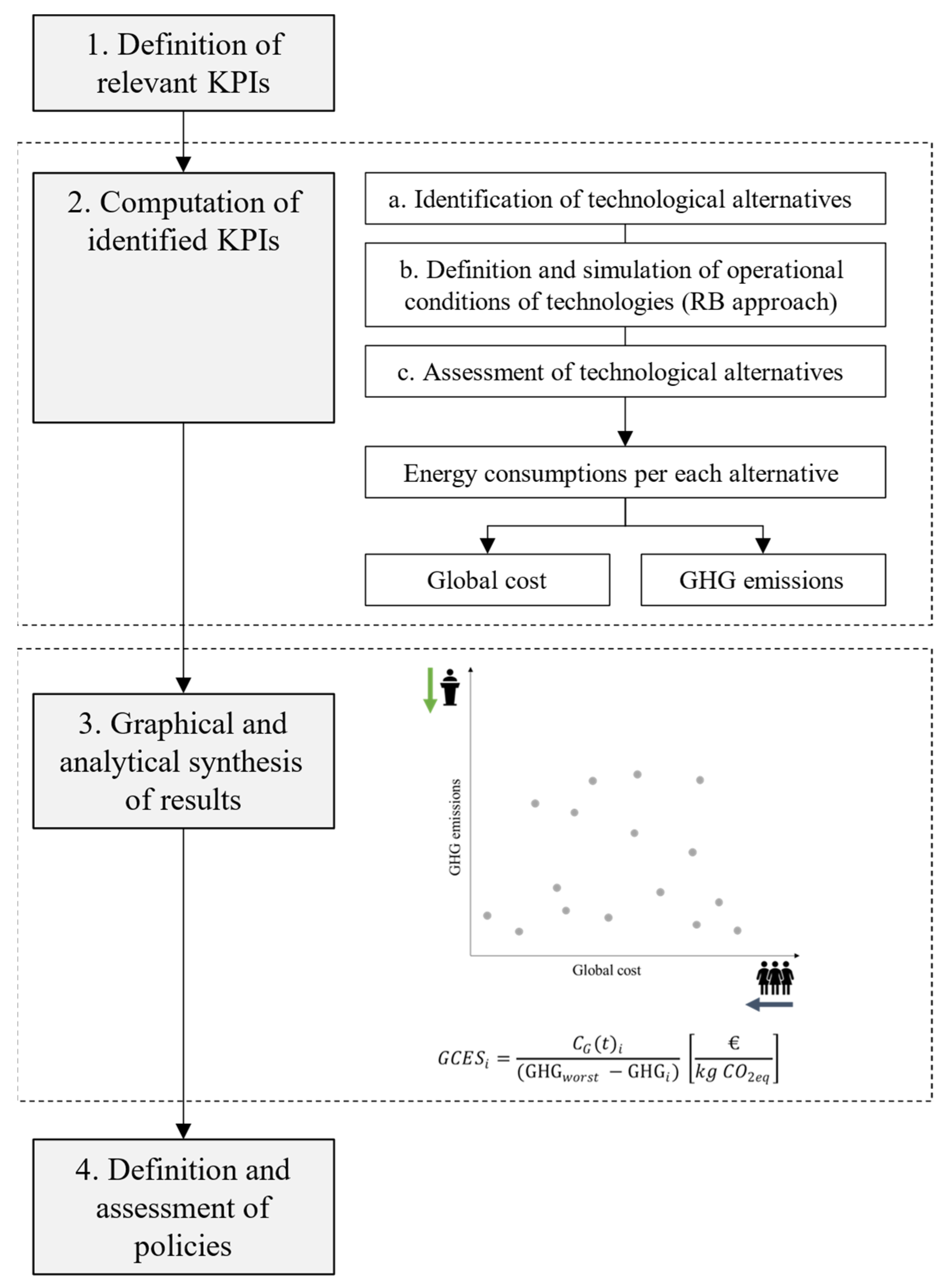
The overall methodology, depicted in Figure 1, is divided into the following steps:

i.

Definition of relevant KPIs: the KPIs are identified to measure financial and environmental performances of a set of generation technologies employed in the building sector;

ii.

Computation of the identified KPIs: the KPIs are computed by making use of the Reference Building (RB) approach;

iii.

Graphical and analytical synthesis of results: KPIs are graphically represented and combined by defining an aggregate indicator (i.e., GCES);

iv.

Definition and assessment of policies: policy measures are defined and assessed in terms of their impacts on the previously introduced GCES indicator.

The methodological steps are further detailed in the following subsections.

2.1. Definition of Relevant KPIs

An effective policy design starts from the knowledge and definition of specific metrics and indicators [27]. Between such indicators, KPIs are defined as indexes aiming to measure the performance of a project, a process, a component, etc., and to monitor its evolution. Thus, their definition needs to be strictly related to the objectives that the analysts want to reach and the aspects they want to control. In the context of this research, KPIs must describe the objectives of the stakeholders involved in the planning of building energy retrofit. In particular, the main perspective of the analysis is the one of the policymakers who, in setting energy policies for buildings, want to have a clear picture of the possibilities and performances of different technologies. On the other side, private investors play a role in technologies spreading, as main owners of buildings. Moreover, by choosing some metrics which can capture possible influencing factors for the next future spreading of the technological alternatives, it is possible to provide an up-to-date snapshot in support of the decision-making process.

With this purpose, two KPIs were selected to measure the performances of the technologies:

• Global cost per square meter [EUR/m²];
• GHG emissions per square meter [kgCO₂eq/m²].

The selected KPIs allow us to represent, respectively, the private and public side drivers in the choice of new technologies to be deployed in building retrofitting. Indeed, as reported in [28], from a private perspective, financial convenience is the main influencing parameter in the process of selecting a new technology to be installed; for this reason, the global cost is designated as an indicator of the financial performance of a particular technology. Global cost is a parameter usually used to compare different alternatives in retrofit interventions. As introduced in the 2010 Energy Performance of Buildings Directive (EPBD) Recast [29], its calculation takes into consideration the initial investment cost of building components and the annual maintenance and operational costs (i.e., mainly energy costs), with the latter discounted at the present value for the entire useful life of the building itself [30]. The same formula can be applied to a single component. By consolidating all expenses incurred by the building owner or occupant, the indicator can assess the financial viability of a technology using a life-cycle approach, serving as a representative measure for making investment decisions [28]. Conversely, GHG emissions are recognized as a potential driver from the perspective of policymakers. It is assumed that, in steering the transition of the building sector toward a low-carbon society, decision makers will formulate appropriate policy measures to incentivize the market’s shift towards adopting low-carbon solutions. The goal is to make these solutions more financially appealing to private entities [28]. Thus, the two identified indicators comprehensively address both private- and public-side objectives when evaluating various technological options for buildings. They enable the capture of factors influencing decision making, ensuring that the results provide a relevant snapshot that remains applicable over the near future.

2.2. Computation of the Identified KPIs

The adoption of a particular technology in buildings guarantees diverse financial and environmental performances, in terms of the above-introduced KPIs. To compute the KPIs, firstly, it is necessary to identify the alternatives to be assessed. To do this, following a market study, the most diffused technologies can be selected, collecting information about their efficiencies and costs for their purchase and maintenance. Also, their typical lifespan (i.e., time after which their replacement is required) needs to be known.

Then, it is fundamental to assess the context in which these technologies would operate, which also influences their financial performance in terms of operational costs (i.e., energy costs). Specifically, the energy needs that these solutions should cover must be estimated. To reduce the computational burden for a large-scale analysis and to better describe the possible boundary conditions of the technology’s operation, the RB approach can be introduced. The RB identifies a real or statistically determined typical building which can be considered representative of a portion of the building stock [31]. Once RBs are developed (i.e., identified and characterized in terms of geometry, thermo-physical properties, periods of construction, and climates), they can be modelled using professional software, and energy needs are calculated based on steady-state or dynamic simulations. Knowing systems efficiencies, an assessment of energy performance for the alternative technologies is conducted via the computation of the annual energy consumption for each technological alternative. More in detail, energy needs are determined via the energy simulations of the RBs, while energy consumption is computed based on the generation, distribution, and emission efficiencies of the alternative technologies. With this approach, the set of technological solutions is applied to the different RBs, consequently leading to diverse energy consumptions. These consumptions are further influenced by the specific characteristics of the RBs themselves. From the resultant final energy consumptions related to the different technologies, global costs and GHG emissions are calculated for each alternative according to the following equations (Equations (1) and (2)).

$$C_G\left(t\right)=C_I+\sum _j[\sum _{i=1}^t\left(C_{a,i}\left(j\right)·R_d\left(i\right)\right)-V_{f,t}\left(j\right)] \left[€\right]$$

(1)

According to EN 15459-1:2017 [30], where $C_I$ corresponds to the initial investment cost [EUR], $C_{a,i}\left(j\right)$ represents the annual costs [EUR/year] (including operation and maintenance) of year i for component j, $R_d\left(i\right)$ the discount formula [-] for year i, and $V_{f,t}\left(j\right)$ is the final value [EUR] of the component j at the end of the calculation period t.

$$GHG=\sum _z{c}_z·E{F}_{GHG,z} \left[\frac{\mathrm{k}{\mathrm{g}}_{\mathrm{C}{\mathrm{O}}_2\mathrm{e}\mathrm{q}}}{\mathrm{y}\mathrm{e}\mathrm{a}\mathrm{r}}\right]$$

(2)

where $c_z$ corresponds to the building final consumption per energy carrier z [kWh/year] and $E{F}_{GHG,z}$ represents the emission factor per energy carrier z [kg_CO2eq/kWh].

Furthermore, given that the emphasis is on a specific technological component, denoted as j, the calculation period t of the $C_G\left(t\right)$ is proportionally aligned with the useful life of the technology, with its final value excluded from the computation.

Thanks to the representativeness of the outcomes of the RB energy models, the results in terms of technologies’ energy performances can be considered as descriptive of a vast portion of the building stock.

2.3. Graphical and Analytical Systemization of the Results

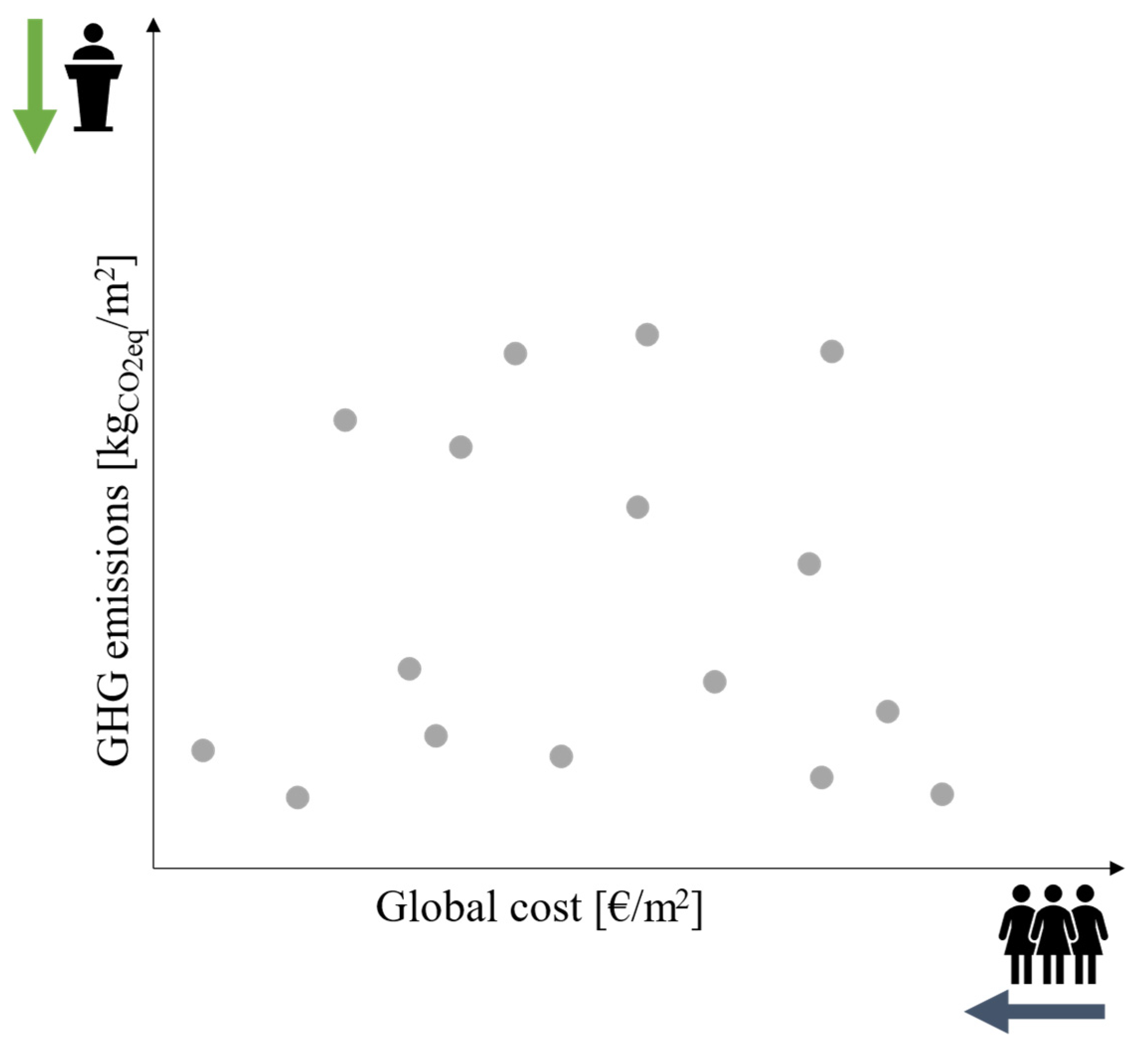
At this point, each technology for each RB is characterized by its unique financial and environmental performance. Moreover, each potential retrofit technology can be compared with the other possible choices for the same operational context (i.e., for the same RB) or under different operational conditions (i.e., if the same technology is adopted in different RBs). To facilitate a visual understanding of the reciprocal behavior of the technologies, the results are synthesized in a graphical tool, as reported in Figure 2.

This graphical representation serves as a policy tool for decision makers, offering a means to assess the interplay of selected technological solutions within the x-y space. It enables a comparative analysis from both financial (private) and environmental (public) perspectives. This graphical tool is particularly interesting for policymakers, allowing them to easily identify the potential risk associated with the adoption of a technology with the worst environmental performance. The representation allows the decision maker to visualize the solutions with the lowest global cost (x-axis), reasonably preferred by private investors, and those with the lowest GHG emissions (y-axis), preferred by public stakeholders, in the view of guaranteeing the achievement of the European goals. It is noteworthy that usually the best solution for the private investor often differs from that of public stakeholders. Going into detail, dots located in the top-right part of the graph represent the worst solutions, characterized by high life-cycle costs and emissions. Conversely, solutions in the bottom-left quadrant are the best, guaranteeing low emissions with minimal financial effort.

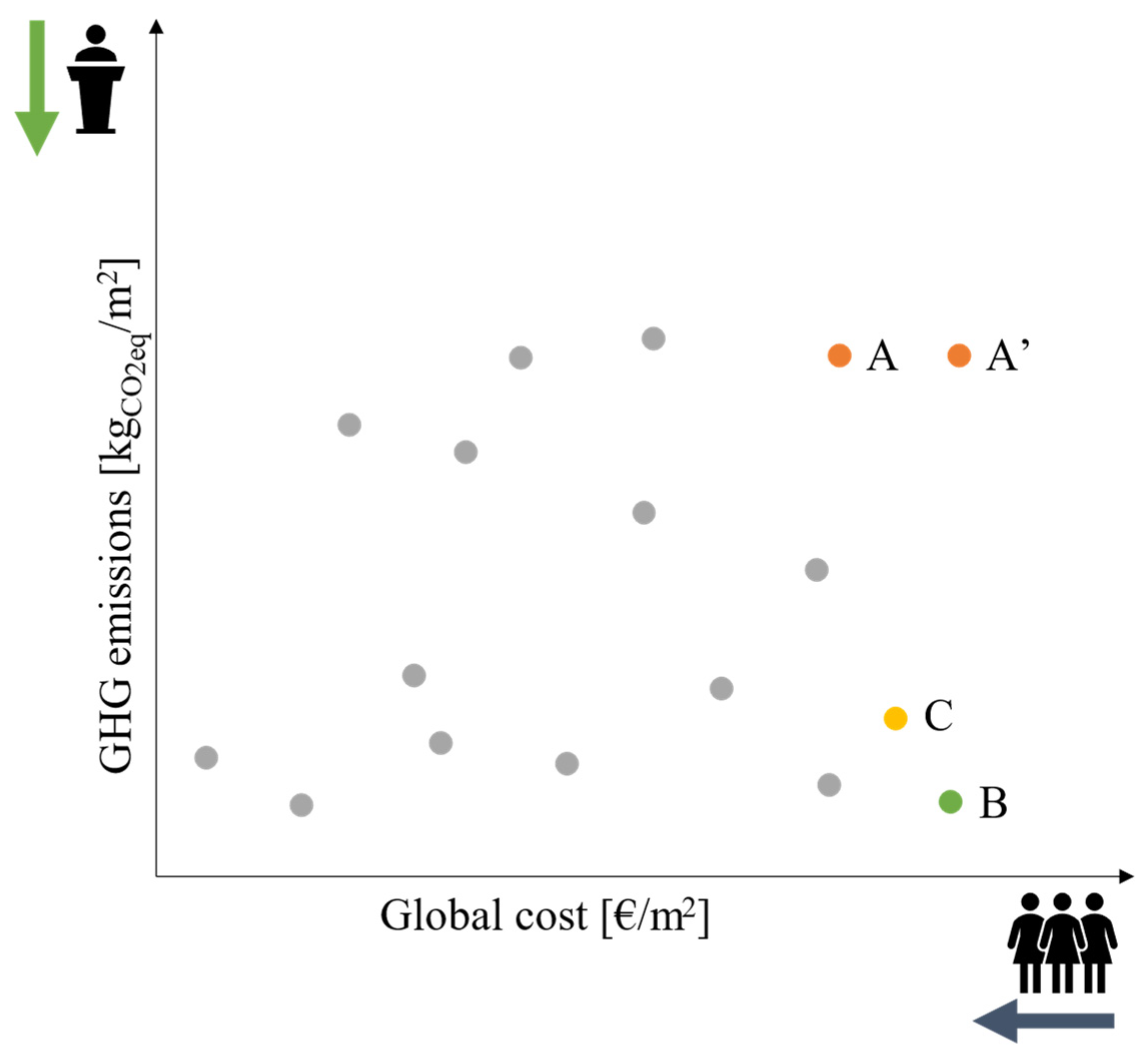
The positioning of the technological solutions is dependent on the RB in which the technology can be installed. For this reason, it becomes crucial to delve into a detailed analysis at the RB scale, facilitating a comparison of alternatives that could potentially replace the existing systems within the same RB. Figure 3 reports an exemplification of two cases in which three technologies (dots A, B, and C in one case; dots A’, B, and C in the other) can be suitable for the retrofit of a specific RB.

In both cases, the graphical tool shows that the represented alternatives are characterized by similar financial performances (i.e., the $C_G\left(t\right)$ index is comparable for the solutions), while their environmental impacts are clearly different (i.e., GHG emissions significantly differ between the alternatives). Indeed, if comparing the first triplet of alternatives (dots A, B, and C), dot A, which represents the most convenient solution from a financial standpoint, is at the same time the worst solution in terms of GHG emissions, while dots B and C are both characterized by lower emissions with respect to A (B has a slightly better environmental performance with respect to C, but against a higher global cost).

Assuming that a private stakeholder would most likely choose based on financial convenience (dot A), this condition represents the highest risk for the policymaker, since it represents the situation in which a private investor would select the solution more environmentally impactful than any other potential alternative at disposal. Differently, in case the least performing solution in terms of GHG emissions is not the most convenient solution from a financial point of view, there is not such a risk. This is the case of A’ in case the solutions for a single RB are represented by dots A’, B, and C (see Figure 3). Therefore, if in this latter case the policymaker would not perceive any risk in the adoption of the most financially attractive solution by the investor (dot C in Figure 3), conversely, in the first case (A, B, and C triplet), she/he would act to push towards more environmentally friendly solutions with proper policy measures.

To tackle this, the GCES aggregate indicator is defined. Specifically, when there is the risk of adoption of the most impactful solution (being financially attractive) from privates (as in the A, B, and C example), GCES is computed for each more environmentally friendly alternative with respect to it, coupling financial and environmental performances at once to study how much the other solutions cost compared to the benefits they guarantee with their adoption in the place of the most impacting option. The indicator is defined as the ratio between the global cost of a competing solution and the GHG emissions that this solution can save with respect to the worst environmentally performing and most financially attractive one, as in Equation (3):

$$GCE{S}_i=\frac{{C_G\left(t\right)}_i}{({GHG}_{worst}-{GHG}_i)} \left[\frac{\mathrm{€}}{\mathrm{k}{\mathrm{g}}_{\mathrm{C}{\mathrm{O}}_2\mathrm{e}\mathrm{q}}}\right]$$

(3)

where ${C_G\left(t\right)}_i$ represents the global cost [EUR] of the i solution among the set of better environmentally performing ones, ${GHG}_{worst}$ represents the emissions of the worst environmentally performing solution, and ${GHG}_i$ represents the emissions of i solution (both expressed in [$\mathrm{k}{\mathrm{g}}_{\mathrm{C}{\mathrm{O}}_2\mathrm{e}\mathrm{q}}$]).

In relation to Figure 3, and according to this vision, considering the first example of technologies potentially applied to a specific RB (dots A, B, and C), dot A would be selected as the worst performing in terms of GHG emissions; thus, it is identified as the benchmark for the assessment of the emissions savings guaranteed by the adoption of the other alternative solutions. The GCES would be then calculated for solutions B (Equation (4)) and C (Equation (5)), dividing their global costs by the emission savings that their adoption could guarantee with respect to a potential adoption of the solution A.

$$GCE{S}_B=\frac{{C_G\left(t\right)}_B}{({GHG}_A-{GHG}_B)} \left[\frac{\mathrm{€}}{\mathrm{k}{\mathrm{g}}_{\mathrm{C}{\mathrm{O}}_2\mathrm{e}\mathrm{q}}}\right]$$

(4)

$$GCE{S}_C=\frac{{C_G\left(t\right)}_C}{({GHG}_A-{GHG}_C)} \left[\frac{\mathrm{€}}{\mathrm{k}{\mathrm{g}}_{\mathrm{C}{\mathrm{O}}_2\mathrm{e}\mathrm{q}}}\right]$$

(5)

In the case of a specific RB, the solution with the lowest global cost is among the most environmentally friendly solutions (as it happens with dots A’, B, and C), where GCES is not computed, and A’ is already excluded for its higher global cost compared to the alternatives.

2.4. Definition and Assessment of Policies

The numerator of GCES, representing global cost, is indicative of investor preferences, whereas the denominator (avoided emissions) reflects the interests of policymakers. Hence, a lower numerator in GCES increases the likelihood of the alternative solution being chosen by the investor. Conversely, a higher denominator makes the solution more favorable to policymakers. Therefore, a low GCES indicator signifies a high likelihood for a technology to gain favor for widespread adoption in the near future, gathering support from both stakeholders. With regard to Figure 3, the indicators computed according to Equations (4) and (5) disclose knowledge about how much technologies B and C cost in relation to the benefit that their adoption would guarantee in terms of emissions savings, if they are chosen by the investor in place of solution A. To make it happen, the policymaker has to translate the environmental benefits in financial terms for the private investor. Therefore, he/she should put in place proper financial measures to make environmentally friendly technologies more likely to be chosen by privates, lowering the GCES indicator of these solutions.

To investigate this issue, based on the graphical decision-support tool, the policymaker can visualize the technologies with the most appealing environmental and financial performances in the baseline situation (i.e., with no new policies in place) and compute GCES. Then, several policy scenarios can be investigated, to understand how these can affect the positioning of the solutions in the graph. In order to achieve this, the policymaker can modify various elements such as market regulation mechanisms or pricing models to evaluate their impact on the baseline GCES aggregate indicator. This assessment is conducted in terms of the percentage variation in GCES for each environmentally friendly solution, prompted by a specific policy scenario. In particular, the analysis aims to explore to what extent the scenarios can have an impact on the global costs associated to each technological alternative. This allows us to forecast how different policies could affect the GCES values, which in turn represent the likelihood of technologies diffusion.

3. Case Study: Italy

The methodology presented in Section 2 was tested on the Italian context to support the decision-making process of retrofit interventions on buildings. The study examined the potential impact of various policies on the likelihood of retrofit technologies’ adoption, considering both the existing situation and alternative policy scenarios. In detail, the focus was on the space heating service, in terms of generation technologies to be adopted for the building retrofit. The reasons behind this application are derived from the statistical data on the energy and environmental impacts of this service [32].

With the aim of providing a policymaker decision-support tool for a mid-term timespan, the computations of the main KPIs were performed for 2030, to provide a forecast of a business-as-usual scenario and of different policy strategies. Specifically, based on a review of the most diffused retrofit options for winter air conditioning in Italy, attention was devoted to three main technological alternatives: condensing gas boiler, biomass boiler, and electric heat pump. Based on the data regarding the main interventions incentivized via the Ecobonus mechanism [33], in 2018, these three technologies represented around 90% of total Ecobonus interventions for winter air conditioning, with condensing gas boilers and heat pumps representing the most diffused ones (67% and 22%, respectively). To characterize the selected alternatives, for each technology, the generation efficiencies were assumed, considering the requirements for the Italian incentive mechanism of Conto Termico 2.0 (i.e., the financial contribute provided in 1, 2, or 5 annual rates for envelope or systems interventions on buildings). In detail, an efficiency of 0.96 was chosen for the gas solution, 0.88–0.89 for the biomass one, and 3.80–4.10 as the COP for electric heat pumps [34].

To compute the energy consumptions, the RB approach was adopted. To develop RBs, the “Typology Approach for Building Stock Energy Assessment” (TABULA) project was taken as an example. It is a European project aimed to develop national building typologies representing the residential building stock of the participating countries [31]. In this application, starting from the TABULA database [35], the RBs were developed and characterized in terms of geometry and envelope properties.

To identify RBs, an initial analysis of the current state of the Italian residential stock was performed, classifying it based on the construction periods and its main typological classes. Indeed, the stock was divided into single-family houses (SFHs) and multi-family houses (MFHs), with the latter being buildings with two or more apartments. SFHs and MFHs were further classified in nine construction periods assumed from the last Italian census [36], as depicted in Figure 4. Grouping the construction periods from ISTAT, three macro-classes were selected, namely “before 1980”, “between 1981 and 2000”, and “after 2001”, connected with the different energy requirements in force in the respective periods. Based on the distribution of SFHs and MFHs in the different construction periods, it was possible to identify the most populated ones within the three defined macro-classes. For each identified construction period, the most relevant RB within the TABULA database was selected as representative of that macro-class for the Italian residential building stock, identifying a total of six RBs (see asterisks in Figure 4).

The six RBs were assumed in terms of geometry and efficiencies of the emission and distribution sub-systems, while they were further characterized in terms of thermal properties. Indeed, due to the lack of data, the RBs defined by the TABULA project are mainly based on data from the Middle Climate zone E (2101 < Heating Degree Days (HDD) < 3000), and more specifically, on the Piedmont region [37]. To tackle the differences in terms of thermal properties of the buildings in the different locations across Italy, TABULA original U-values were adjusted in accordance with [38]. In the referenced report, comprehensive information is presented regarding prevalent building constructions and their corresponding thermal transmittances across different eras and construction types. From the ISTAT database [36], data detailing the quantity of buildings corresponding to each building type and construction period within various climatic zones were extracted. By combining the information from both reports, average Italian U-values were computed via a weighted process, according to the frequency distribution of the main construction elements found in SFHs and MFHs for each period across the entire country (see

Table 1. Average Italian U-values of the main construction typologies of the RBs. Elaborated from [36,38].

Construction Typology	U-Value [W/m2K]
	Before 1980	1981–2000	After 2001
Floor	1.48	1.34	0.85
Ceiling	1.61	1.19	0.71
External vertical walls	1.28	1.05	0.73
External glazed surfaces	3.74	3.54	3.20

).

Finally, based on the ISTAT classification [36], the six RBs were further diversified to evaluate the effects of climate conditions on buildings’ energy needs, considering five geographical zones (North–West, North–East, Center, South, and Islands). Globally, the Italian building stock was assumed to be represented by 30 RBs (six RBs across five zones).

Once fully characterized, the resulting RBs were modelled via quasi steady-state simulations, using MasterClima 11300 software v. 2.27. The climate conditions of Turin, Venice, Rome, Bari, and Palermo were used and, from the simulations, energy needs for space heating were obtained. Then, according to the technical characteristics of the technologies to be assessed (i.e., generation efficiencies), energy consumptions were computed, assuming the efficiencies of the other subsystems (distribution and emission) constant (defined in accordance with TABULA [35]). For each RB, starting from the computation of the energy consumptions, global costs, and GHG emissions were assessed per each technology, according to Equations (1) and (2), assuming the techno-economic parameters reported in

Table 2. Techno-financial parameters of the technological options for space heating system interventions [34].

Technology	Typical Lifetime	Investment Cost [EUR/kW] *	Annual Maintenance Cost [%]
Condensing gas boiler	20 years	100–137	1.5
Biomass boiler	20 years	460–570	2
Electric heat pump	20 years	580–644	3

* Investment cost is maintained as constant during the timespan and is equal to current market values.

. Specifically, investment costs were derived from a review of main price lists in Italy, while annual maintenance costs were assumed as percentage values of the initial investment costs, as defined by Annex A of EN 15459-1:2017 [30]. Emission factors were extracted from [39,40].

To be consistent with the choice of the 2030 timespan, prices of domestic energy commodities (i.e., natural gas, biomass, and electricity) and electricity emission factors (dependent on the power mix) were varied based on IEA projections [3]. Specifically, for the energy prices, IEA growth rates were applied to 2015 price statistics for gas, biomass, and electricity (chosen as the reference year in accordance with [34]). Both electricity and gas prices were dependent on consumption bands. A particular attention was devoted to the electricity price, varying according to tariff schemes. Indeed, it is important to consider that, in 2015, a voluntary tariff experimentation for heat pumps was underway, aiming to render heat pumps more competitive on the market [41]. The experimentation, valid only for autonomous systems using a heat pump as the sole heating system, considered the adoption of a non-progressive tariff for electricity (i.e., not dependent on actual consumption and equal to 0.170 EUR/kWh), in substitution of the existing variable one. The convenience of the tariff was strictly related to the annual electricity consumption of the buildings; the greater the consumptions, the more convenient the tariff was. Indeed, for consumption higher than 1800 kWh/year, the tariff was 0.244 EUR/kWh, while for lower consumption, it was 0.123 EUR/kWh. Hence, for all the representative buildings (RBs) equipped with autonomous heating systems, the model employed for global cost calculation automatically opted for tariff experimentation only if it proved to be more cost effective than the regular pricing scheme. What was reported so far allowed us to depict a baseline scenario, providing a snapshot of the financial and environmental performances of the selected technologies in 2030. According to this scenario, it becomes possible to pinpoint the least environmentally friendly solution and calculate the $GCES$ index for each alternative within every RB.

The calculated $GCES$ indicators are strongly dependent on the defined boundary conditions (incentive mechanisms, taxes, contract formulation, etc.). Therefore, different elements in terms of market regulation mechanisms and pricing models were investigated to explore their impact on the global costs associated to each technological alternative, and thus, to study how different policies could affect the $GCES$ values. In total, six policy scenarios were identified and compared with the baseline. Three scenarios aimed to include, into the global cost formulation, the incentive mechanisms, already present in the Italian context in 2015, but not accounted in the traditional global cost calculation. Specifically, two measures were considered: Ecobonus (i.e., 10-years-based tax rebate for buildings’ retrofit computed as percentage of the investment cost) and Conto Termico 2.0. In detail, the ECO policy scenario considered the adoption of the Ecobonus for the three technologies, as envisioned by Italian regulation, while the CT policy scenario considered the adoption of the Conto Termico 2.0 only for electric heat pumps and biomass generators, with gas technologies excluded from this mechanism. To make heat pumps more competitive in terms of global cost, with respect to traditional technologies, the INC scenario considered the adoption of the actual incentive mechanisms (Ecobonus or Conto Termico 2.0, according to which is more advantageous for the different applications) only for electric heat pumps.

Another analysis (the TF scenario) was carried out in relation to energy price formulations. Aligned with the current regulations, which have recently eliminated the progressive nature of electricity prices, the envisioned scenario uses a uniform variable electricity price. This price is set as equal to the lowest rate applicable to residential consumers, regardless of the type of heating system (autonomous or centralized) [41].

Finally, the introduction of environmental taxes was studied, intending to translate environmental costs into financial burdens for private investors. Attention was paid to taxation of both GHG (in terms of CO₂eq) and PM emissions, thus dealing also with the issue of local air pollution, which represents a crucial concern especially in urban areas, where the concentration of pollutants is drastically increasing. Due to the severe consequences that these harmful pollutants can have on health, local governments should promote adequate policies and precautions to prevent serious consequences on people’s health and the environment. In the building sector, fuel combustion for heating purposes represents the major source of air pollutants’ emissions. In line with this, two additional scenarios were developed:

• Scenario TXC, which considered the adoption of a taxation on the CO₂eq emissions produced using space heating systems;
• Scenario TXPM, which assumed the adoption of a taxation on the PM10 emissions produced using space heating systems.

The values derived from [42] were differentiated for SFHs and MFHs according to the estimation of their percentage consumptions over the stock [37].

The cited policy scenarios and their main assumptions are summarized in

Table 3. Policy scenarios and main assumptions.

Scenario	Incentives	Environmental Costs	Price Modulation
BASE	None	None	Non-progressive tariff for autonomous heat pumps according to real convenience
ECO	Ecobonus	None	Non-progressive tariff for autonomous heat pumps according to real convenience
CT	Conto Termico 2.0	None	Non-progressive tariff for autonomous heat pumps according to real convenience
INC	Ecobonus or Conto Termico 2.0	None	Non-progressive tariff for autonomous heat pumps according to real convenience
TF	None	None	Non-progressive tariff for all systems
TXC	None	CO2eq taxation for space heating systems	Non-progressive tariff for autonomous heat pumps according to real convenience
TXPM	None	PM10 taxation for space heating systems	Non-progressive tariff for autonomous heat pumps according to real convenience

, where the voices in italics represent the assumptions characteristic of each alternative policy scenario.

4. Results and Discussion

This section presents the outcomes of the application of the methodology for the comparison of a set of existing technologies suitable for the retrofit of space heating generation systems in the Italian case study. The results aim to guide and support decision makers in evaluating the current state of technologies performances and in formulating appropriate strategies and policy measures to potentially drive individuals’ choices towards low-carbon solutions. According to the methodological steps, this section is structured as follows: Section 4.1 analyzes the graphical decision-support tool developed to make the decision maker aware of the environmental and financial performances of each identified technology. Then, Section 4.2 reports the $GCES$ percentage variations in each technology, with respect to the baseline, considering the six alternative policy scenarios (reflected in the boundary conditions of the calculation), concerning different incentive measures, market regulation mechanisms, or pricing models (Table 3). Furthermore, a comparison of the $GCES$ between the two more eco-friendly technologies is presented in Section 4.3, expressed as $\mathrm{\Delta }GCES$. This additional perspective offers insight, allowing the decision maker to visually apprehend the alterations in the competitive dynamics among the technologies induced by each alternative policy scenario.

4.1. Graphical and Analytical Systemization of the Results

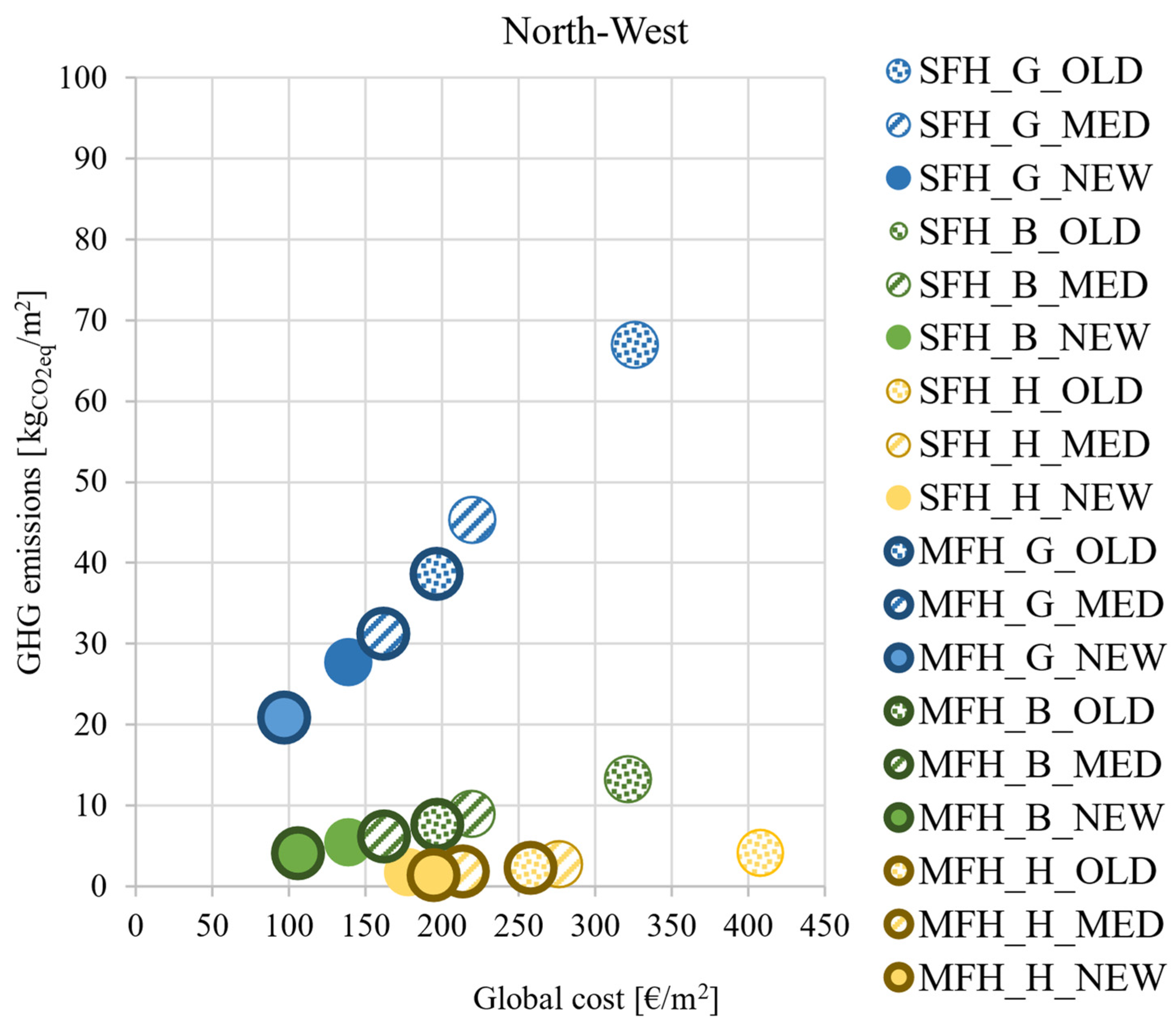
The graphical decision-support tool, presented in the scatterplot of Figure 5, is intended to allow the decision maker to have an overall snapshot of the financial and environmental performances of the technological solutions that can be used in case of retrofit interventions of the thermal generator on different RBs in the same geographical area. Indeed, a general overview of the positioning of the technologies in the graph allows a policymaker to be aware of the operational conditions of the RBs in their area of interest/competence, to potentially identify priorities of intervention on the stock, and to better tailor future policy strategies and interventions on the local stock conditions. Furthermore, attention must be paid to the technologies potentially applicable to the same RB (each characterized by specific features in terms of geometry, thermal properties, typology, construction period, and climate). In this paper, as previously explained, three thermal generation technologies were defined as potential alternatives in the case of retrofit: condensing gas boiler, biomass boiler, and electric heat pump. For exemplification purposes, Figure 5 shows the results for the North–West of Italy. Specifically, each “triplet” of technological solutions is represented in Figure 5 for the six RBs in North–West (for a total of 18 dots), each identified by the same filling and edge of the dots. In detail, the filling represents the construction period, while the edge is used to differentiate SFHs and MFHs; specifically, dots with no edge represent the SFHs, while the ones with the solid edge are the MFHs. Finally, the colour is used to indicate the possible retrofit solution (i.e., blue for gas, green for biomass, and yellow for heat pump).

Analyzing the two KPIs separately, it comes out that, for each RB, the condensing gas boiler (blue dots) is the solution with the worst environmental performance, compared to the other two competing technologies. From the financial standpoint, instead, it appears that the solution with the lowest global cost (among the ones potentially considered for the specific RB retrofit) does not always coincide with the most environmentally risky. Depending on the RB, biomass boiler and condensing gas boiler are highly competitive, while heat pump is always characterized by the highest global cost, due to its higher investment and operational costs.

As explained in Section 2.2, only for the RBs in which the solution with the worst environmental performance (i.e., condensing gas boiler) coincides with the most financially attractive for the investors, the GCES aggregate indicator is calculated, according to Equation (3). The aim is to evaluate how much the other solutions (biomass boiler and electric heat pump) cost in relation to the benefit that their adoption would guarantee in terms of GHG emissions’ savings with respect to the gas solution, which nowadays is the most widely deployed in the residential sector [32,38]. Looking at Figure 5, this situation in the North–West area occurs for all MFHs and for the SFHs built after 2001 (of which potential retrofits are identified by SFH_H_NEW, SFH_G_NEW, and SFH_B_NEW in the graph). The results can differ depending on the geographical area, which influences the operational conditions of the retrofit solutions, and thus, their reciprocal behavior.

The GCES is computed for alternative solutions, exhibiting superior environmental performance compared to the condensing gas boiler. Among these, the most advantageous solutions are those marked by the lowest aggregate indicators, signifying technologies that offer substantial GHG emissions savings relative to the most financially competitive alternative. Regarding the outcomes of the GCES calculation for the baseline scenario (hereinafter referred to as BASE), it is evident that, across all RBs where GCES is computed, the biomass boiler consistently presents the lowest aggregate indicator (see

Table 4. GCES values for SFHs [EUR/kgCO₂eq].

		North–West	North–East	Center	South	Islands
Before 1980	Biomass boiler		5.98		6.93	7.36
	Heat pump		6.50		7.57	8.17
1981–2000	Biomass boiler		6.08		7.14	7.70
	Heat pump		6.57		7.73	8.45
After 2001	Biomass boiler	6.25	6.33	7.39	7.66	8.43
	Heat pump	6.85	6.96	8.24	8.55	8.58

and

Table 5. GCES values for MFHs [EUR/kgCO₂eq].

		North–West	North–East	Center	South	Islands
Before 1980	Biomass boiler	6.36	6.43		7.83	8.61
	Heat pump	7.10	7.24		7.97	9.33
1981–2000	Biomass boiler	6.46	6.51		8.06	9.19
	Heat pump	7.26	7.39		8.35	10.27
After 2001	Biomass boiler	6.31	6.39	7.63	8.09	11.02
	Heat pump	9.95	10.10	11.97	12.64	13.11

). This suggests that the biomass boiler technology appears to yield the most favourable GCES in comparison to the gas alternative. In the tables, the empty cells represent situations in which GCES was not computed.

4.2. Evaluation of the Effect of Different Financial Policies

To increase the competitiveness of a technology in terms of GCES, the aim is to minimize the aggregate indicator by lowering the numerator (global cost), with the denominator being fixed by buildings operations and systems efficiencies. Therefore, as said in Section 3, six policy scenarios were proposed, to explore the effect of different market regulation mechanisms and pricing models on the aggregate indicator.

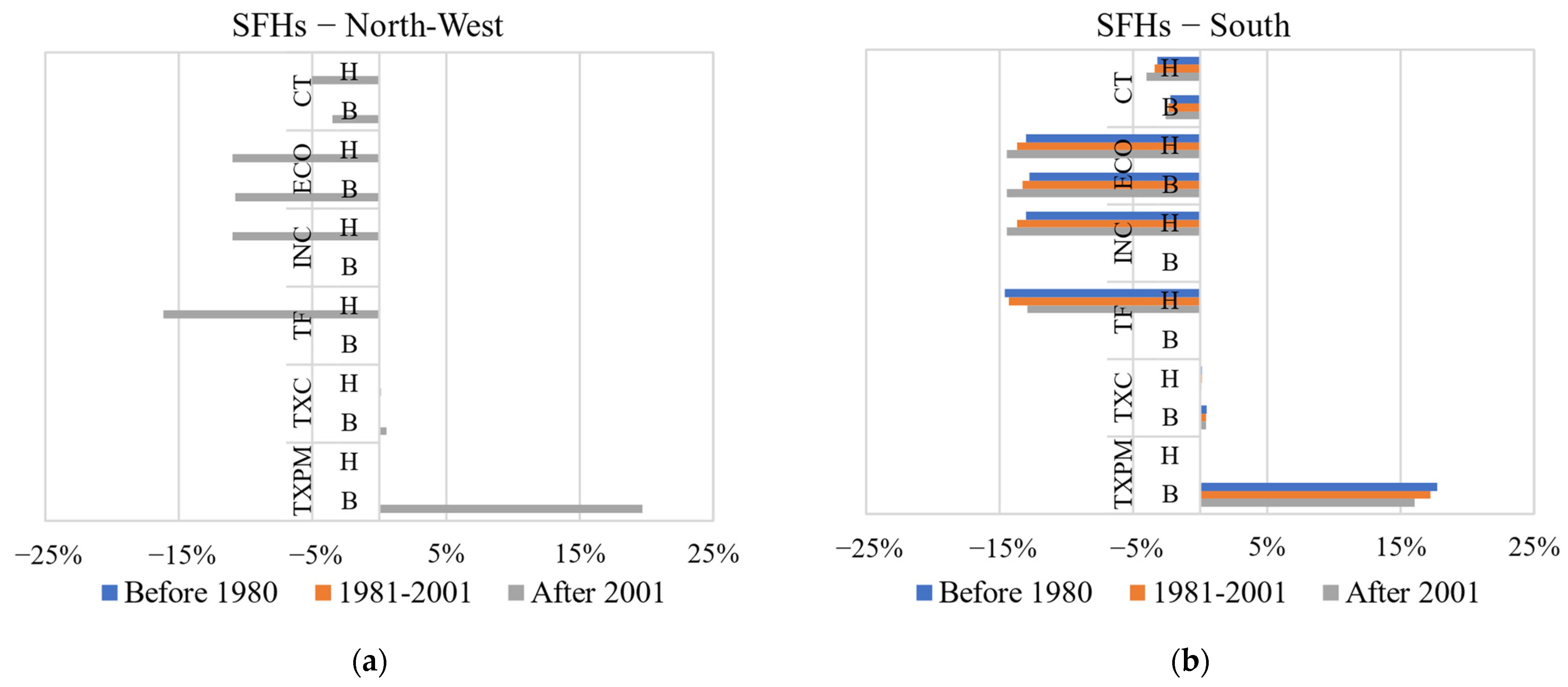
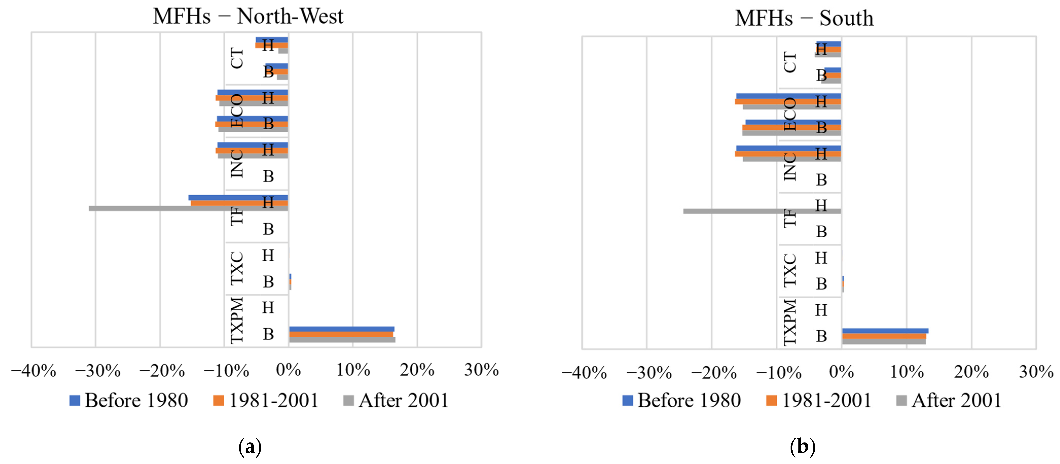
In this regard, a first analysis aimed to evaluate the percentage variation that each policy measure causes on the GCES of the two environmentally friendly solutions (when computed), with respect to the BASE scenario. The following figures (Figure 6 and Figure 7) summarize the results of this evaluation. Specifically, a negative value means that the applied policy lowers the GCES by decreasing the global cost of the considered technologies. The results are presented for SFHs and MFHs located in North–West and South, in order to exemplify how the reciprocal behavior of the solutions can be dependent on the location.

As expected, the only positive variations are experienced in the TXPM and TXC scenarios, since they induce an overall increase in the global costs of the considered technologies by applying specific taxations on the PM and CO₂eq emissions. If, on the one hand, the TXC scenario has a low impact on the GCES, with the CO₂eq emissions being small for both technologies, on the other hand, the TXPM scenario presents a greater percentage variation for the biomass boiler, since this technology is the largest PM emitter among the considered ones. Indeed, taking SFHs in the Southern area as an example (Figure 6b), the TXC scenario provokes a maximum positive GCES percentage variation of +0.48% for the biomass boiler and +0.11% for the heat pump, while the TXPM scenario leads to a maximum variation in the aggregate indicator as equal to +17.74% and +0.04%, concerning the biomass and the electric solutions, respectively. It is trivial that these scenarios are not making biomass and heat pumps technologies more financially appealing in absolute terms. However, their reciprocal performance changes, as will be commented on later.

Focusing on the other scenarios, by definition, TF only affects the global cost of the heat pump solution. Considering the SFHs, the percentage variation in GCES for the TF scenario is always negative, as can be seen in Figure 6a,b for North–West and South, respectively, meaning that the policy is able to induce a reduction in the overall heat pump global cost. Indeed, the simulated annual SFHs consumptions are always greater than 1800 kWh/y (this consideration is valid for all the considered geographical zones, with the sole exception of SFHs built after 2001 and located in the Islands area). Therefore, in the BASE scenario, the model for the calculation of the global cost independently selects the most convenient electricity tariff, which is the voluntary tariff experimentation, which in turn is higher than the non-progressive tariff proposed in the TF scenario. Coming to MFHs, the results for the TF scenario are more dependent on the location. In the reported graphical examples, it is possible to note that a reasoning similar to that of SFHs can be made for the MFHs in North–West (Figure 7a), for all the RBs built before 2001 (the same result is observable for North–East). On the contrary, the same MFHs located in South (Figure 7b) present consumptions lower than 1800 kWh/y and, therefore, the TF scenario has no influence on the GCES results, since the considered electricity tariff in the TF scenario is identical to that already considered in the BASE scenario. The same trend reported in Figure 7b can be noticed for the Center and Islands geographical areas. Finally, a separate deepening is required for the MFHs built after 2001, which represent exceptions for both presented geographical areas. This RB is the sole among the considered ones with a centralized heating system and, in case of heat pump adoption, has high electricity consumptions (>1800 kWh/y), where it cannot access the heat pump experimental tariff in the BASE scenario, paying for the highest energy price. For this reason, as shown in Figure 7, for this RB, either in North–West or South, the TF scenario presents the highest negative GCES percentage variation with respect to the BASE for the electric heat pump, meaning that this policy scenario is capable of inducing a huge decrease in the heat pump global cost, thanks to the strong reduction in the energy cost. In detail, for the MFHs located in the South of Italy, the TF scenario leads to a GCES percentage variation of −24.41%, while in North–West, the variation in the aggregate indicator reaches −31.02%.

ECO and CT scenarios concern the introduction of incentive mechanisms into the global cost formulations, considering separately the application of Ecobonus and Conto Termico 2.0 on both biomass boiler and heat pump. Since no incentives were considered in the BASE scenario, both ECO and CT scenarios result in negative percentage variations in the aggregate indicators. Detailing the comparison between the two instruments, it appears that the Ecobonus scheme provides a higher decrement of the global cost than Conto Termico 2.0 for both technologies, for both SFHs and MFHs. Deepening this aspect, the ECO scenario provokes a variation that is at least twice the variation in the CT scenario; in fact, in the reported example of the South case study, for all SFHs and for MFHs, the percentage variation in the ECO scenario for biomass boiler is almost five times the value resulting from the CT scenario, and at least 3.5 times when considering the heat pump technology. Moreover, it is possible to note from the figures that the ECO scenario leads to similar percentage values for biomass boilers and heat pumps, while the CT one slightly advantages the heat pump over the biomass boiler. Finally, the INC scenario considers the adoption of the most convenient incentive mechanism (among Conto Termico 2.0 and Ecobonus) only for the electric heat pump, thus contributing to GCES variations with respect to the BASE scenario only for heat pumps. As for ECO and CT scenarios, the effect of the INC scenario can only be a reduction in the global cost of the heat pump solution, thus producing a negative percentage GCES variation for this solution.

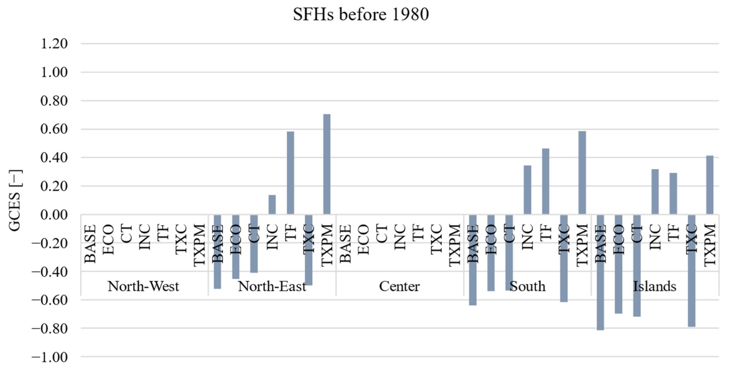
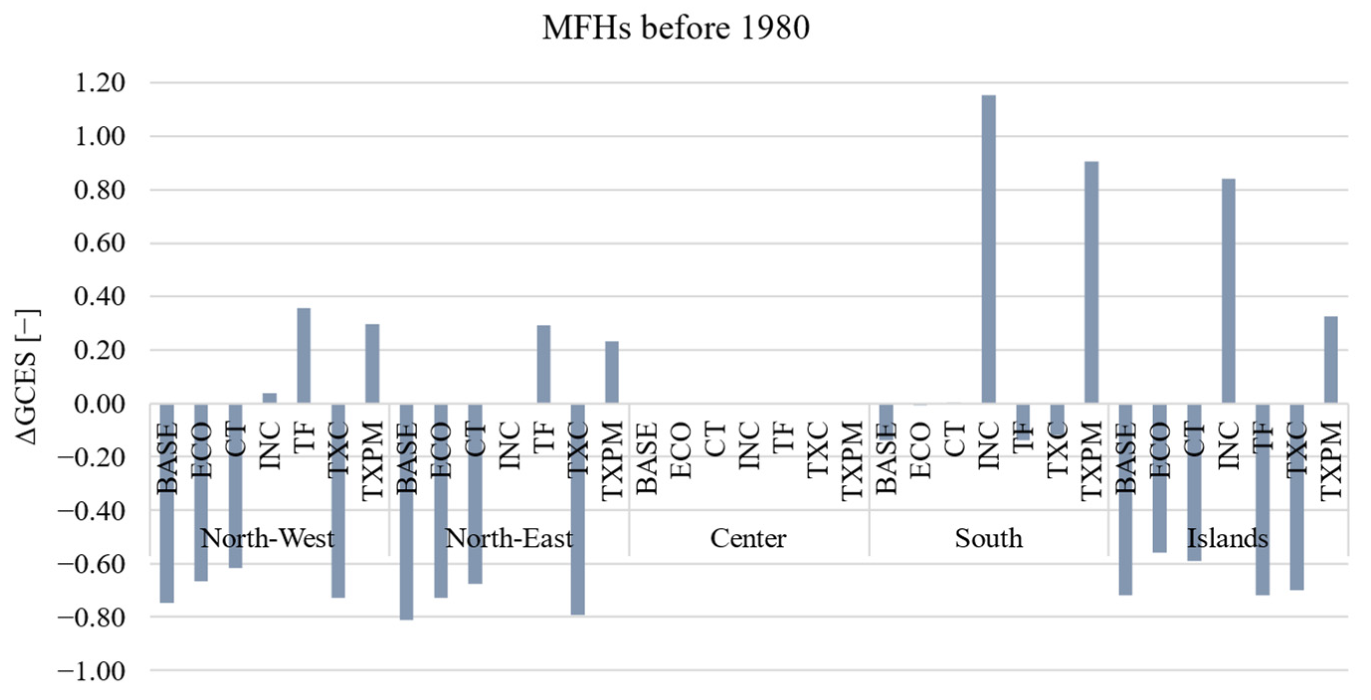
4.3. Computation of ΔGCES

After the analysis of the effects that each policy scenario has on the GCES of the single technology, it is interesting to provide information on the relative competition between the different technological solutions. In this application, for the cases in which GCES is computed, the “green” technologies in competition with the condensing gas boiler are only two, thus allowing for the calculation of the ΔGCES index, which is defined as the difference between the GCES indicators of the biomass boiler (${GCES}_B$) and of the heat pump (${GCES}_H$), for the same RB, as shown in Equation (6).

$$\mathrm{\Delta }GCES={GCES}_B-{GCES}_H$$

(6)

By definition, a positive value of the $\mathrm{\Delta }GCES$ represents a greater advantage in choosing heat pump as a retrofit technology over biomass, while a negative value means that the biomass boiler leads to major benefits. As mentioned earlier, this step facilitates the creation of a graphical representation illustrating the mutual competition between the biomass boiler and electric heat pump. This visualization aids policymakers in easily comprehending how the implementation of a specific policy might influence the market, steering it towards one technology over the other. As an exemplification of the results, Figure 8 and Figure 9 depict the outcomes of the $\mathrm{\Delta }GCES$ values’ computation (for the cases in which GCES calculation was performed) for SFHs and MFHs built before 1980.

At first glance, it can be noticed that, accordingly to the GCES outcomes, the BASE scenario is characterized by negative $\mathrm{\Delta }GCES$ values, since the biomass boiler appears to be the most competitive retrofit solution in all the RBs for which GCES was computed. Figure 8 and Figure 9 allow for visualizing which of the policy scenarios are able to guarantee the greatest variations in the competition between the two technologies, with respect to the initial situation represented by the BASE condition.

Firstly, it is possible to note that ECO and CT scenarios present $\mathrm{\Delta }GCES$ values close to the BASE ones. This is because the two policies provide incentives in a comparable way to the two technologies. Thus, even though the incentives affect the GCES of each technology, the proportion between the variation in the aggregate indicators is similar for biomass boiler and heat pump for the same RB, resulting in a little variation in the delta between them, thus still advantaging biomass.

Despite the fact that they do not contribute to lowering the GCES index for heat pumps and biomass generators, scenario TXC and TXPM can affect their relative competitiveness. However, looking at the figures, it can be observed that the TXC scenario also presents almost no variation in the $\mathrm{\Delta }GCES$ with respect to the BASE case, since both technologies emit low CO₂eq emissions, and thus, this taxation has a small impact on the GCES values. Conversely, a different behavior is linked to the application of the TXPM scenario. The biomass boiler is the major PM emitter compared to the heat pump (approximately an 80:1 ratio between biomass and electricity PM emission factors [39,40]). This issue provokes a great imbalance in terms of aggregate indicators of the two competing technologies, boosting the electric retrofit solution. In this regard, Figure 8 and Figure 9 highlight that the $\mathrm{\Delta }GCES$ of the TXPM scenario, for both SFHs and MFHs and for all the presented geographical zones, changes in sign, becoming positive with respect to the BASE scenario. Therefore, this results in a change in the ranking of the technologies, advantaging heat pumps over biomass generators.

Finally, INC and TF scenarios deal with measures that only affect the heat pump option. In this context, it can be stated that for the RBs with low energy consumptions, the incidence of the cost of energy decreases, and thus, the other components of the global cost (i.e., incentive mechanisms) gain weight. For this reason, for Islands in SFHs and for South and Islands in MFH, where RBs present low annual consumptions, the INC scenario is the one which leads to the greatest positive differences in terms of $\mathrm{\Delta }GCES$ values since it is able to advantage heat pumps over biomass boilers to the greatest extent. On the other hand, when energy consumption is high, the weight of the energy cost on the global cost is greater; therefore, the policy scenario inducing the biggest changes compared to the BASE case is the one that affects the cost of electricity (i.e., TF scenario), as it can be observed for the SFHs in North–East and South, and for the MFHs in North–West and North–East. In addition to the observed trend, it is interesting to focus on the priority changes. Indeed, if for the SFHs, the abolition of the progressive tariff for electricity (as envisaged by the TF scenario) results in a variation in priority between biomass boiler and heat pump with respect to BASE (from negative to positive $\mathrm{\Delta }GCES$ values), different considerations must be drawn for MFHs. In those cases, it emerges that the $\mathrm{\Delta }GCES$ for the TF scenario is positive only for North–West and North–East zones, while for South and Islands, it is possible to observe a preference of biomass boiler ($\mathrm{\Delta }GCES$ values are still negative, as in the BASE scenario). This trend is related to the electricity tariffs. Indeed, in regions where the annual electricity consumption is higher than 1800 kWh/y (as in North–West and North–East), the application of the new non-progressive tariff is convenient and is able to lower the global cost of the heat pump, making the electric technology more convenient (thus resulting in a ${GCES}_H$ lower than the associated ${GCES}_B$), as what happened in the SFHs. Conversely, in case the annual consumptions are lower than 1800 kWh/y (i.e., South and Islands), the considered energy tariff for the global cost calculation is identical in the BASE and TF scenarios, and thus, in these cases, there is not a variation in the ranking between the heat pump and the biomass boiler.

In conclusion, the main implication of this study is that, via the examination of various graphical tools, decision makers can promptly discern which measures have the potential to bring about tangible changes in technology competitiveness. For instance, if the decision maker aims to promote electric technologies for the emission reduction and integration of renewable sources, the focus would be on enhancing the attractiveness of heat pumps. This can be achieved by either reducing the overall cost of the technology itself, such as by influencing energy costs (i.e., the TF Scenario), by promoting incentives (i.e., the INC Scenario), or by increasing the cost of the competing technology, for example, by impacting local emissions taxation (i.e., the TXPM Scenario). Utilizing the findings from this analysis, in addition to identifying the policies that lead to its objective, the policymaker is also able to understand on which types of buildings one intervention may be more effective than another and then quantify its effects.

5. Conclusions

Efforts to meet ambitious targets in the building sector are crucial due to its significant societal and environmental impacts. With an estimated 75% of the European building stock considered energy inefficient, the primary challenge lies in renovating existing buildings to realize environmental and financial benefits. Various approaches, including the use of Key Performance Indicators (KPIs), are employed to evaluate and support building renovation programs. KPIs facilitate the setting and monitoring of medium- and long-term objectives, translating data into actionable insights for policymakers. The development of tailored metrics allows for a comprehensive assessment, addressing both financial and non-financial aspects of building stock renovation.

Keeping this in mind, in the following, it is possible to summarize the key findings of the study:

• Decision-making support tools, in the form of graphical and analytical instruments, were defined to provide a forecast of the effects of a business-as-usual scenario and of alternative policy instruments on the reciprocal convenience of different technologies, focusing on thermal generators for space heating in residential buildings.
• The paper contributes to the definition of proper KPIs to assess the building performances from a multi-dimensional standpoint and to the conceptualization of a methodological framework in support of decision-making process in energy planning for buildings.
• The definition of the new aggregate GCES indicator permitted to stress on the importance of integrating different perspectives into the study of building retrofit options, highlighting how private (financial) and public (environmental) objectives are usually contrasting among them. Low GCES values indicate high likelihood for the technology to see its diffusion, since it represents a good tradeoff between both private and public sides. Based on the definition of the GCES, the analysis of the alternative policy scenarios allowed us to investigate how policymakers should evaluate how different policy schemes or instruments could help in translating the environmental benefits of some technological solutions into financial burdens for investors, thus guiding the adoption of more environmentally friendly solutions. Indeed, the analysis allowed us to explore how potential future policies, in terms of market regulation mechanisms or pricing models, could affect the GCES values, and thus, could influence the likelihood of technologies’ diffusion.
• In the Italian application, it was possible to observe that under the baseline scenario (BASE), biomass boiler was advantageous against heat pump, according to the ΔGCES index. Scenarios ECO, CT, INC (dealing with technology-specific incentives), and TXC (introducing a tax based on GHG emissions) were not able to change the technological ranking, with heat pumps still not being competitive enough in financial terms. With the TXPM scenario, instead, heat pumps turned out to be the most financially appealing alternative, penalizing the high PM emissions caused by biomass boilers. In some areas, the same effect was guaranteed also by the TF scenario (dealing with a change in the tariff schema for electricity), while in others, it was not, underling how important is to have ad-hoc policy measures for specific circumstances.

Future Perspectives

The paper opens the way to future possible research. Despite the encountered difficulties in terms of data availability, the methodology could be potentially extended to different contexts. The application to the Italian case study, in addition to the limitations due to the reduced number of technological alternatives compared, represents a clear exemplification of the developed methodological framework, which can be further deepened. Indeed, future work could be developed for investigating different technological solutions, as well as other end-uses (e.g., space cooling, domestic hot water, etc.). Even though it would be interesting to apply the methodological steps also to the non-residential buildings, the scarcity of appropriate RBs for this building category may make it still difficult to explore. Additionally, the same methodology can also be employed to develop indicators different from the one reported in the application. Depending on the decision maker’s objectives, various perspectives related to the energy, environmental, and/or financial aspects of the building system can be considered (e.g., PM emissions instead of CO₂eq). In this paper, the authors chose to report the GCES indicator because, currently, CO₂ is one of the major drivers in policy decisions.

Finally, the methodological approach introduced in this paper could be implemented as the basis for the development of future scenarios of technological diffusion at national or regional scales, using the indicator of likelihood of technology diffusion as a discriminant for deep national renovation scenarios.