
Subsea Long-Duration Energy Storage for Integration with Offshore Wind Farms


Abstract
1. Introduction
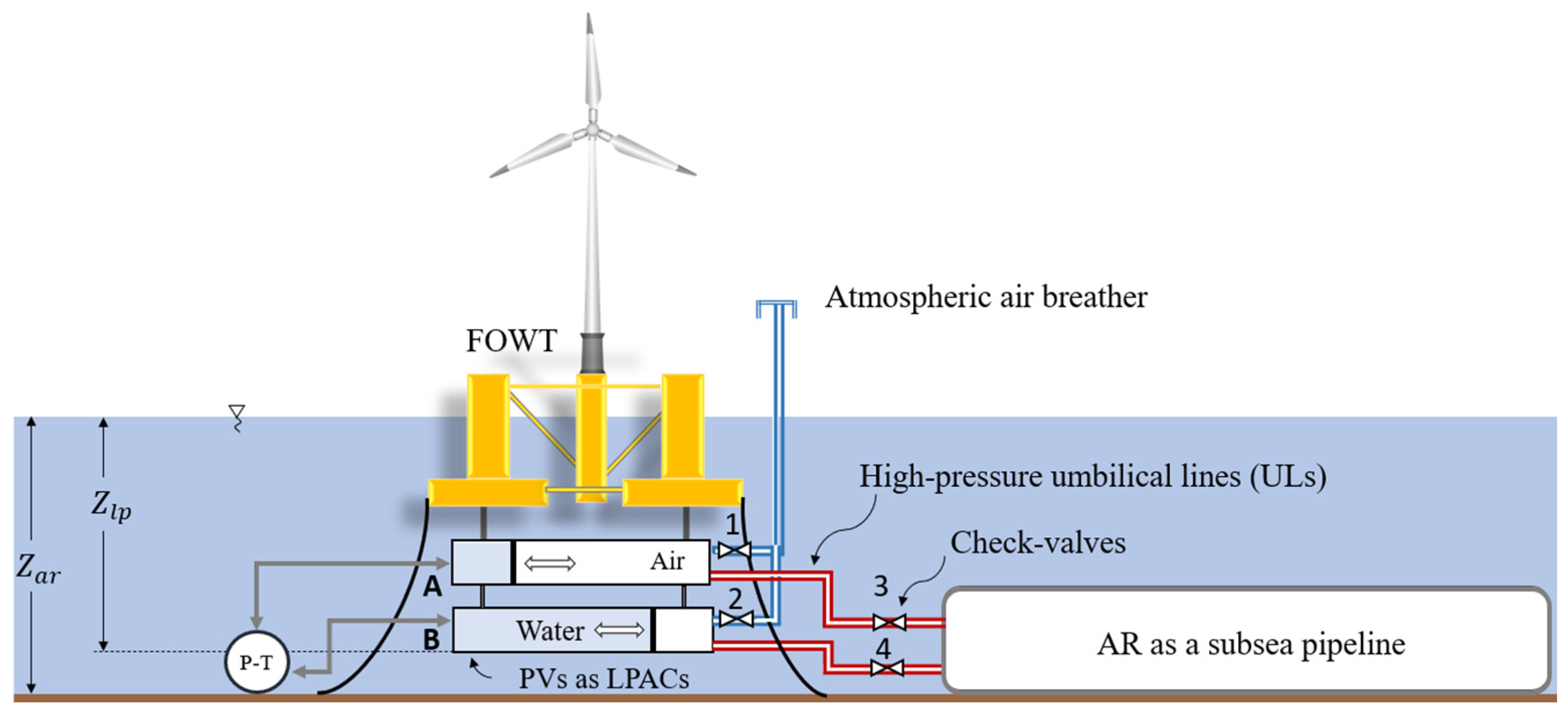
2. Conceptual Model
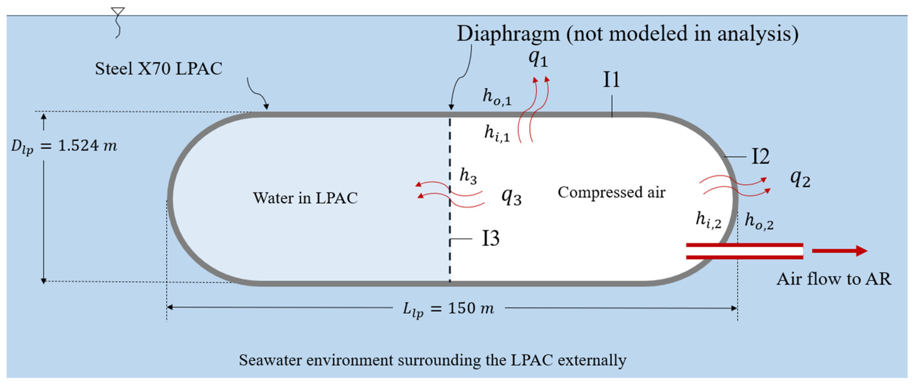
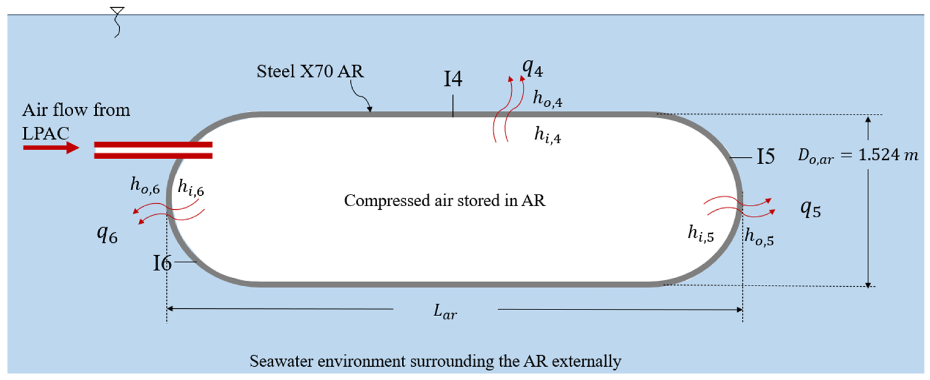
3. Proposed Mathematical Model for Simulating Thermal Performance
3.1. Mass Conservation
3.2. Energy Conservation
3.3. The Bernoulli Equation Along the UL
3.4. Key Performance Indicators (KPIs)
4. Numerical Model
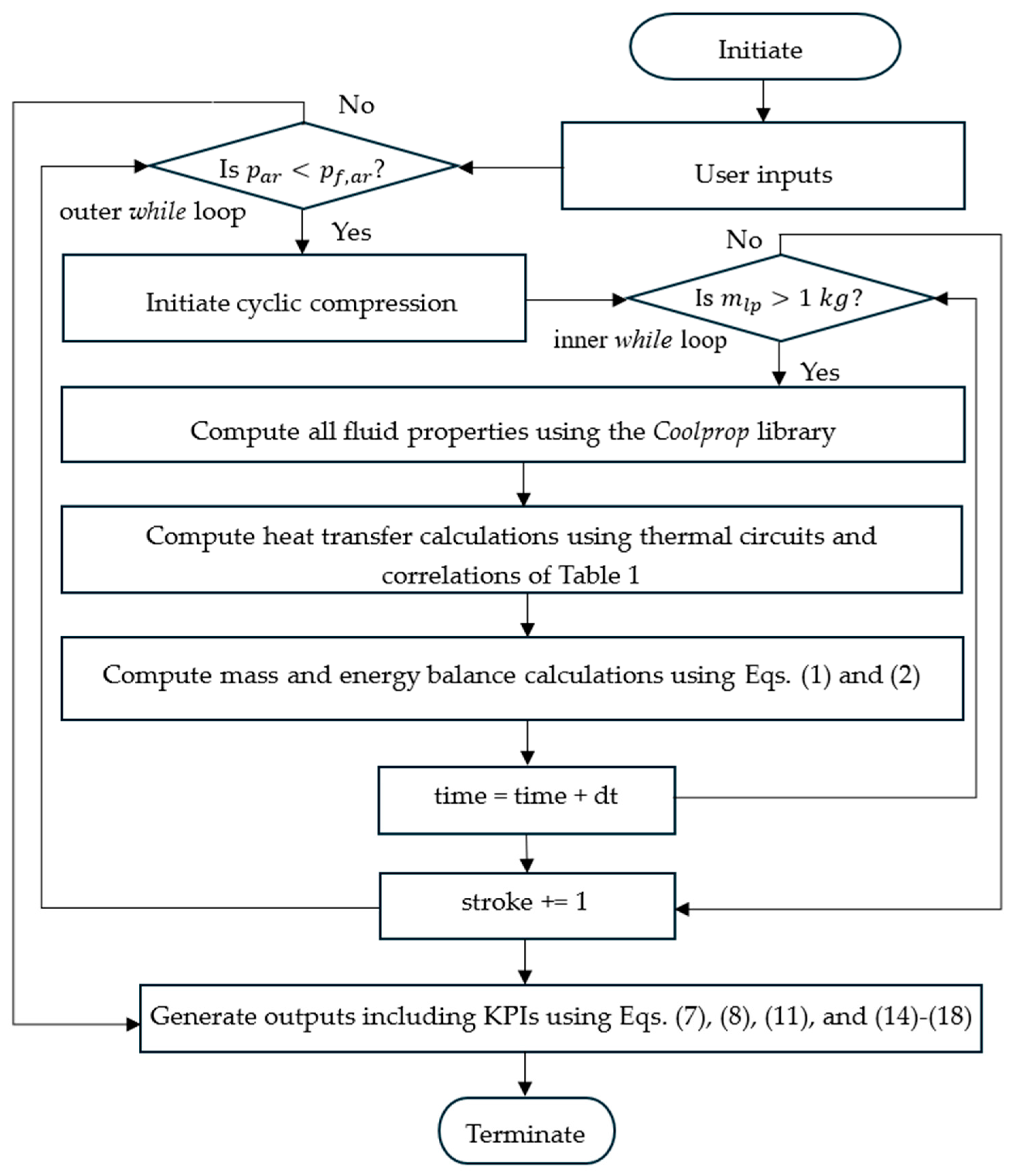
4.1. Program Description
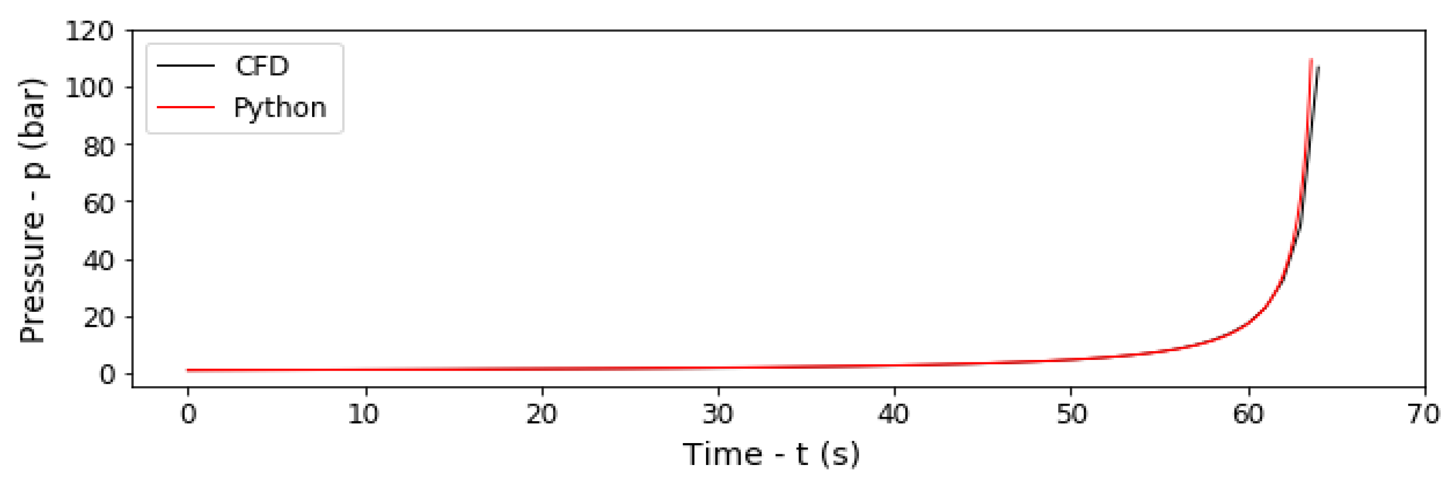
4.2. Program Validation
5. Results
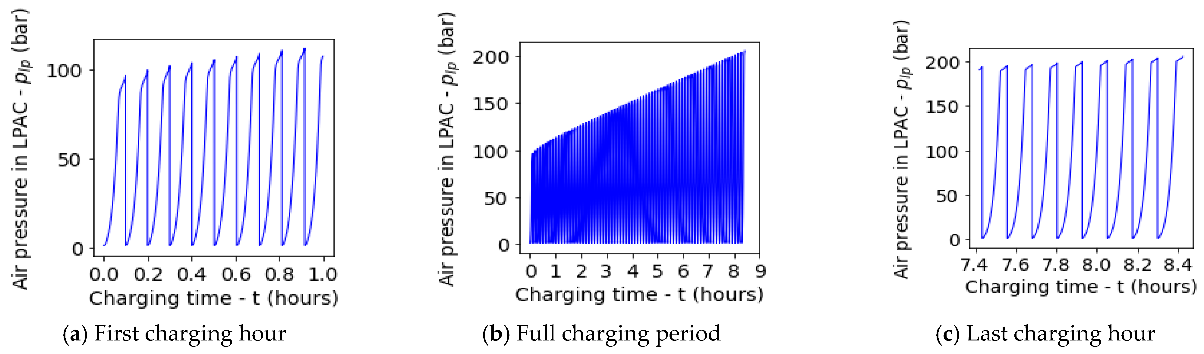
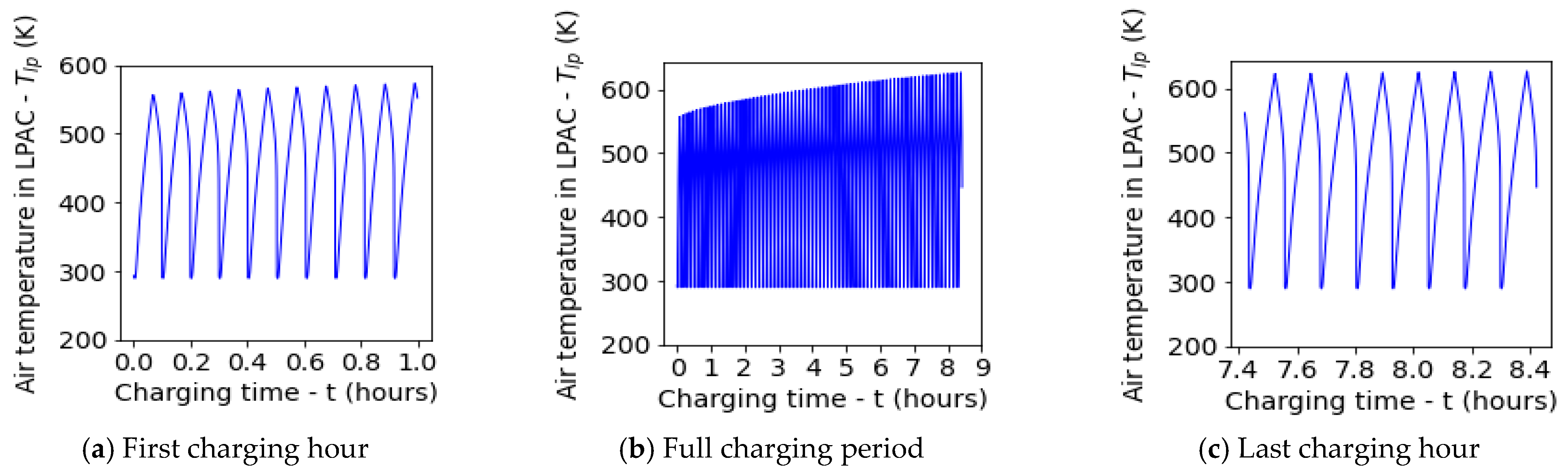
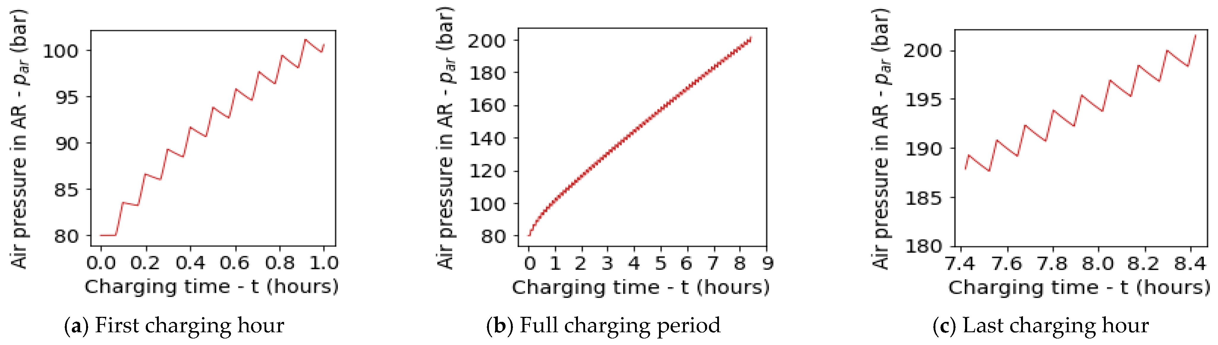
5.1. Default Test Run
5.2. Parametric Study
6. Conclusions
- i.
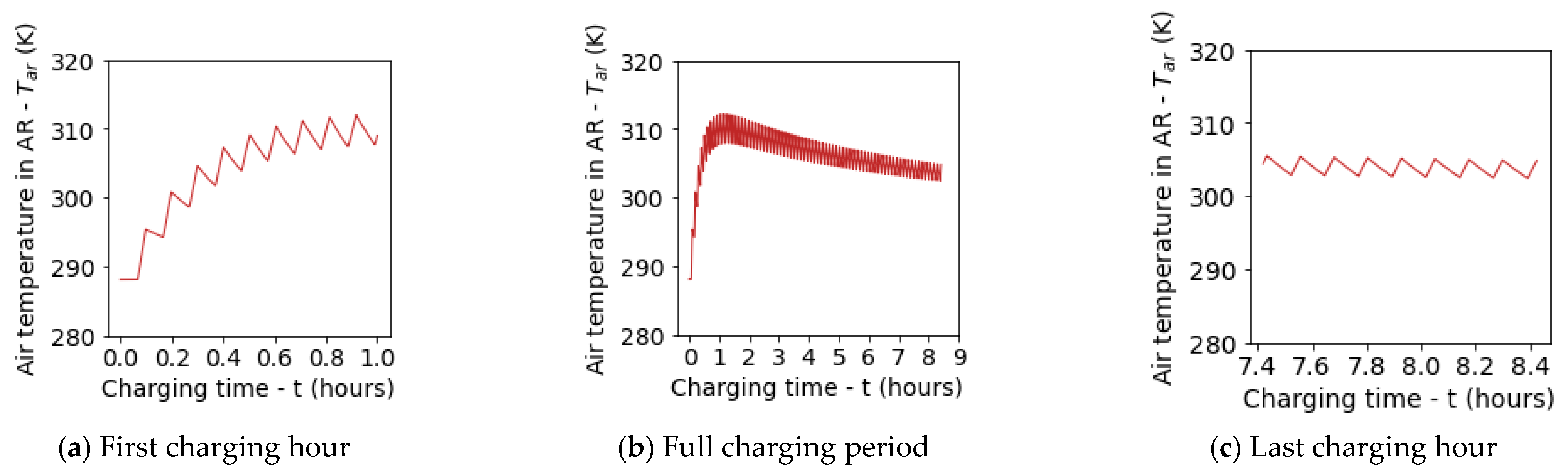
- The LDES system will take over 8 h to charge a 2500 kWh subsea AR to 200 bar peak pressure. This finding is subject to the test conditions including the geometric and operating conditions of the LPACs;
- ii.
- Notwithstanding the use of slender LPACs located subsea, the cyclic compression deviates substantially from the ideal, isothermal conditions. The maximum polytropic index was predicted to reach a value of 1.17, leading to compressed air temperatures in the LPACs that exceed 600 K.
- i.
- ii.
- The augmentation factor for the ESD of an O-HPES system with respect to a C-HPES system falls in the range of 2.00 and 8.10. The actual augmentation value of a given system depends on whether the calculation of the ESD for the O-HPES system accounts for the volume of the AR only or the volume of the AR and LPACs;
- iii.
- The ESD of an O-HPES system was estimated to reach 16.20 kWh/m3 when based on the volume of the AR only. When the volume of the LPACs was also considered, the ESD reached was found to drop to approximately 4–9 kWh/m3, depending on the volumetric capacity of the AR;
- iv.
- When changing the geometry of the AR, a trade-off between the WR and ESCR occurs. That is, if a change in geometry causes the WR to increase, the ESCR decreases, and vice-versa;
- v.
- The variations in WR and ESCR with a change in Lar/Do,ar up to a factor of 20 were found to not exceed 10%;
- vi.
- Lowering the input hydraulic power for a given LPAC geometry is a key aspect to simultaneously improve both the WR and ESCR of the O-HPES system;
- vii.
- Subject to the test conditions considered in this study, a WR higher than 0.80 and an ESCR above 0.95 are technically achievable when the O-HPES is allowed to charge slowly over a period of 30 h (i.e., 1.25 days).
Author Contributions
Funding
Data Availability Statement
Conflicts of Interest
Abbreviations
| AR | Air Receiver |
| CAES | Compressed Air Energy Storage |
| CFD | Computational Fluid Dynamics |
| C-HPES | Closed-cycle Hydro-pneumatic Energy Storage |
| CP | Compression Phase |
| CV(s) | Control Volume(s) |
| ESC | Energy Storage Capacity |
| ESCR | Energy Storage Capacity Ratio |
| ESD | Energy Storage Density |
| ESDR | Energy Storage Density Ratio |
| KPI(s) | Key Performance Indicator(s) |
| LDES | Long-duration Energy Storage |
| LHS | Left-hand Side |
| LP | Liquid piston |
| LPAC(s) | Liquid-piston Air Compressor(s) |
| MSL | Mean Seawater Level |
| FOWT(s) | Floating Offshore Wind Turbine(s) |
| HPES | Hydro-pneumatic Energy Storage |
| HTC(s) | Heat Transfer Coefficient(s) |
| O-HPES | Open-cycle Hydro-pneumatic Energy Storage |
| P-T | Pump-turbine |
| RE | Renewable Energy |
| RHS | Right-hand Side |
| ROPES | Repurposing Offshore Pipelines for Energy Storage |
| RSP | Release and Storage Phase |
| UL | Umbilical Line |
| WR | Work ratio |
References
- Hywind Tampen. Available online: https://www.equinor.com/energy/hywind-tampen (accessed on 12 November 2024).
- Gomes, J.G.; Lin, Y.; Jiang, J.; Yan, N.; Dai, S.; Yang, T. Review of Offshore Wind Projects Status: New Approach of Floating Turbines. In Proceedings of the 5th International Conference on Power and Energy Applications, Guangzhou, China, 18–20 November 2022. [Google Scholar]
- Our Offshore Wind Farms. Ørsted. Available online: https://orsted.com/en/what-we-do/renewable-energy-solutions/offshore-wind (accessed on 12 November 2024).
- Enabling Large-Scale Offshore Energy Storage, FLASC—Renewable Energy Storage. Available online: https://offshoreenergystorage.com/ (accessed on 14 November 2024).
- Odukomaiya, A.; Abu-Heiba, A.; Graham, S.; Momen, A.M. Experimental and Analytical Evaluation of a Hydro-pneumatic Compressed-Air Ground-Level Integrated Diverse Energy Storage (GLIDES) System. Appl. Energy 2018, 221, 75–85. [Google Scholar] [CrossRef]
- Hydrostor. Available online: https://www.hydrostor.ca/ (accessed on 17 November 2024).
- Ess Iron Flow Chemistry, ESS, Inc. Available online: https://essinc.com/iron-flow-chemistry/ (accessed on 17 November 2024).
- Technology, Highview Power. Available online: https://highviewpower.com/technology/ (accessed on 17 November 2024).
- Olympios, A.V.; McTigue, J.D.; Farres-Antunez, P.; Tafone, A.; Romagnoli, A.; Li, Y.; Ding, Y.; Steinmann, W.D.; Wang, L.; Chen, H.; et al. Progress and Prospects of Thermo-mechanical Energy Storage—A Critical Review. Prog. Energy 2021, 3, 022001. [Google Scholar] [CrossRef]
- Chen, H.; Peng, Y.; Wang, Y.; Zhang, J. Thermodynamic Analysis of an Open Type Isothermal Compressed Air Energy Storage System based on Hydraulic pump/turbine and Spray Cooling. Energy Convers. Manag. 2020, 204, 112293. [Google Scholar] [CrossRef]
- Li, C.; Wang, H.; He, X.; Zhang, Y. Experimental and Thermodynamic Investigation on Isothermal Performance of Large-scaled Liquid Piston. Energy 2022, 249, 123731. [Google Scholar] [CrossRef]
- He, X.; Wang, H.; Sun, H.; Huang, Y.; Wang, Z.; Ling, L. Thermodynamic Investigation of Variable-Speed Compression Unit in Near-Isothermal Compressed Air Energy Storage. Energy Storage 2023, 5, e481. [Google Scholar] [CrossRef]
- Pimm, A.J.; Garvey, S.D.; de Jong, M. Design and testing of Energy Bags for underwater compressed air energy storage. Energy 2014, 66, 496–508. [Google Scholar] [CrossRef]
- Wang, Z.; Xiong, W.; Ting, D.S.K.; Carriveau, R.; Wang, Z. Conventional and advanced exergy analyses of an underwater compressed air energy storage system. Appl. Energy 2016, 180, 810–822. [Google Scholar] [CrossRef]
- Dick, C.; Puchta, M.; Bard, J. StEnSea–Results from the pilot test at Lake Constance. J. Energy Storage 2021, 42, 103083. [Google Scholar] [CrossRef]
- Buhagiar, D.; Sant, T.; Farrugia, R.N. Marine Testing of a Small-scale Prototype of the FLASC Offshore Energy Storage System. In Proceedings of the 6th Offshore Energy and Storage Summit, Brest, France, 10–12 July 2019. [Google Scholar]
- Wiley, W.; Bergua, R.; Robertson, A.; Jonkman, J.; Wang, L.; Borg, M.; Fowler, M. Definition of the Stiesdal Offshore TetraSpar Floating Wind System for OC6 Phase IV; Rep. No. NREL/TP-5700-86442; National Renewable Energy Laboratories: Golden, CO, USA, 2023. [Google Scholar]
- Hazim, A.S.; Buhagiar, D.; Gray, A. Repurpose Offshore Pipeline as Energy Storage ROPES: Opening a New Market Segment Offshore. In Proceedings of the Offshore Technology Conference, Houston, TX, USA, 25–26 October 2022. [Google Scholar]
- Whitaker, S. Forced Convection Heat Transfer Correlation for Flow in Pipes, Past Flat Plates, Single Cylinders, Single Spheres, and for Flow in Packed Beds and Tube Bundles. AIChE J. 1972, 18, 361. [Google Scholar] [CrossRef]
- Gnielinski, V. New Equations for Heat and Mass Transfer in Turbulent Pipe and Channel Flow. Int. Chem. Eng. 1976, 16, 359–368. [Google Scholar]
- Haaland, S.E. Simple and Explicit Formulas for the Friction Factor in Turbulent Pipe Flow. J. Fluids Eng. 1983, 105, 89–90. [Google Scholar] [CrossRef]
- Churchill, S.W.; Chu, H.H.S. Correlation Equations for Laminar and Turbulent Free Convection from a Horizontal Cylinder. Int. J. Heat Mass Transf. 1975, 18, 1049–1053. [Google Scholar] [CrossRef]
- Churchill, S.W.; Bernstein, M.A. Correlating Equation for Forced Convection from Gases and Liquids to a Circular Cylinder in Crossflow. J. Heat Transf. 1977, 99, 300–306. [Google Scholar] [CrossRef]
- Lewandoski, W.; Kubski, P.; Khubeiz, J.M.; Bieszk, H.; Wilczewski, T.; Szymański, S. Theoretical and Experimental Study of Natural Convection Heat Transfer from Isothermal hemispheres. Int. J. Heat Mass Transf. 1997, 40, 101–109. [Google Scholar] [CrossRef]
- Ludovisi, D.; Garza, I.A. Natural Convection Heat Transfer in Horizontal Cylindrical Cavities: A Computational Fluid Dynamics (CFD) Investigation. In Proceedings of the ASME 2013 Power Conference, Boston, MA, USA, 29 July–1 August 2013. [Google Scholar]
- Shiina, Y.; Fujimura, K.; Akino, N.; Kunugi, T. Natural Convection Heat Transfer in Hemisphere. JNST 1988, 25, 254–262. [Google Scholar] [CrossRef]
- Incropera, F.P.; Dewitt, D.P.; Bergman, T.L.; Lavine, A.S. Fundamentals of Heat and Mass Transfer, 6th ed.; John Wiley and Sons: Hoboken, NJ, USA, 2007. [Google Scholar]
- Welcome to Python.org, Python. Available online: https://www.python.org/ (accessed on 19 November 2024).
- Ansys Inc. Ansys Fluent. Available online: https://www.ansys.com/products/fluids/ansys-fluent (accessed on 21 November 2024).
- Canada’s Oil and Natural Gas Producers (CAPP). Use of High Density Polyethylene (HDPE) Lined Pipelines; Canada’s Oil and Natural Gas Producers (CAPP): Calgary, AB, Canada, 2022. [Google Scholar]
- Li, L.; Fu, J.; Yao, Y.; Wang, X.; Liu, K.; Han, T.; Han, B. Generation mechanism of lack of fusion in X70 steel welded joint by fully automatic welding under steep slope conditions based on numerical simulation of flow field. JAMT 2023, 126, 4055–4072. [Google Scholar] [CrossRef]
- White, F.M. Fluid Mechanics, 7th ed.; McGraw-Hill: New York, NY, USA, 2009. [Google Scholar]


| Location | Type of Convection | HTC | Correlation/Fixed Value | Source |
|---|---|---|---|---|
| External | Natural | Churchill-Chu [22] | ||
| External | Forced | Churchill-Bernstein [23] | ||
| External | Natural | Lewandoski et al. [24] | ||
| External | Forced | Whitaker [19] | ||
| Internal | Natural | Ludovisi-Garza [25] | ||
| Internal | Forced | Gnielinski [20] | ||
| Internal | Natural | Shiina et al. [26] | ||
| Internal | Forced | 100 W/m2 K | [27] | |
| Internal | Natural/Forced | 200 W/m2 K | [11] |
| Parameter (Unit) | Value |
|---|---|
| Maximum hydraulic power— (kW) | 5.50 |
| Geometric cylindrical length— (m) | 7.55 |
| Outer diameter— (m) | 0.080 |
| Inner diameter— (m) | 0.075 |
| Volumetric capacity— (m3) | 0.033 |
| Initial air pressure— (bar) | 1 |
| Maximum final operating pressure— (bar) | 100 |
| Initial air temperature— (K) | 293.15 |
| Parameter (Unit) | LPACs | AR |
|---|---|---|
| Hydraulic power— (kW) | 420 | N/A |
| Geometric cylindrical length— (m) | 149.44 | 95.04 |
| Outer diameter— (m) | 1.524 | 1.524 |
| Inner diameter— (m) | 1.420 | 1.430 |
| Volumetric capacity— (m3) | 237.69 | 154.53 |
| Internal surface roughness— (m) [30] | 4 × 10⁻⁵ | 4 × 10⁻⁵ |
| Thermal conductivity— (W/ m K) [31] | 64 | 64 |
| Specific heat capacity of steel— (J/kg K) [31] | 480 | 480 |
| Vertical depth below MSL— (m) | 10.50 | 200 |
| Initial air pressure— (bar) | 1 | 80 |
| Maximum final operating pressure— (bar) | 200 | 200 |
| Design pressure— (bar) | 220 | 220 |
| Initial air temperature— (K) | 293.15 | 288.15 |
| Initial external seawater temperature— (K) | 293.15 | 288.15 |
| Initial internal seawater temperature— (K) | 293.15 | N/A |
| Initial steel temperature— (K) | 293.15 | 288.15 |
| Parameter (Unit) | UL |
|---|---|
| Geometric length— (m) | 190 |
| Inner diameter of umbilical— (m) | 0.05 |
| Internal surface roughness— (m) [30] | 4 × 10⁻⁵ |
| Secondary loss coefficient—sudden expansion— (-) [32] | 0.998 |
| Secondary loss coefficient—sudden contraction— (-) [32] | 0.499 |
| Secondary loss coefficient—valves— (-) [32] | 2 |
| Secondary loss coefficient—bends— (-) [32] | 0.3 |
| Number of valves— (-) | 1 |
| Number of bends— (-) | 2 |
| Test Case | Input Power (kW) | Ideal ESC of AR (kWh) | Ideal ESD 1 of System (kWh/m3) | Ideal ESD 2 of System (kWh/m3) | Volumetric Capacity of AR (m3) | Outer Diameter of AR (m) | Length of AR (m) | Length-to-Diameter Ratio of AR (-) |
|---|---|---|---|---|---|---|---|---|
| A (Default) | 420 | 2500 | 16.20 | 3.97 | 154 | 1.52 | 95 | 62.5 |
| B | 420 | 2500 | 16.20 | 3.97 | 154 | 0.76 | 387 | 509.2 |
| C | 420 | 2500 | 16.20 | 3.97 | 154 | 2.03 | 53 | 26.1 |
| D | 105 | 2500 | 16.20 | 3.97 | 154 | 1.52 | 95 | 62.5 |
| E | 420 | 5000 | 16.20 | 6.37 | 309 | 1.52 | 191 | 125.7 |
| F | 420 | 10,000 | 16.20 | 9.14 | 618 | 1.52 | 383 | 252.0 |
| Test Case | Time to Fully Charge the AR (hrs) | Number of LP Strokes (-) | Maximum Polytropic Index (-) | Maximum Air Temperature in LPACs (K) | Work Ratio WR (-) | ESCR or ESCD (-) |
|---|---|---|---|---|---|---|
| A (Default) | 8.4 | 74 | 1.17 | 626.6 | 0.72 | 0.85 |
| B | 8.7 | 77 | 1.17 | 626.3 | 0.69 | 0.90 |
| C | 8.1 | 71 | 1.17 | 626.3 | 0.75 | 0.80 |
| D | 30.8 | 79 | 1.08 | 436.1 | 0.80 | 0.94 |
| E | 17.4 | 153 | 1.17 | 627.0 | 0.70 | 0.89 |
| F | 35.5 | 313 | 1.17 | 627.1 | 0.68 | 0.92 |
Disclaimer/Publisher’s Note: The statements, opinions and data contained in all publications are solely those of the individual author(s) and contributor(s) and not of MDPI and/or the editor(s). MDPI and/or the editor(s) disclaim responsibility for any injury to people or property resulting from any ideas, methods, instructions or products referred to in the content. |
© 2024 by the authors. Licensee MDPI, Basel, Switzerland. This article is an open access article distributed under the terms and conditions of the Creative Commons Attribution (CC BY) license (https://creativecommons.org/licenses/by/4.0/).
Share and Cite
Cutajar, C.; Sant, T.; Aquilina, L.; Buhagiar, D.; Baldacchino, D. Subsea Long-Duration Energy Storage for Integration with Offshore Wind Farms. Energies 2024, 17, 6405. https://doi.org/10.3390/en17246405
Cutajar C, Sant T, Aquilina L, Buhagiar D, Baldacchino D. Subsea Long-Duration Energy Storage for Integration with Offshore Wind Farms. Energies. 2024; 17(24):6405. https://doi.org/10.3390/en17246405
Chicago/Turabian StyleCutajar, Charise, Tonio Sant, Luke Aquilina, Daniel Buhagiar, and Daniel Baldacchino. 2024. "Subsea Long-Duration Energy Storage for Integration with Offshore Wind Farms" Energies 17, no. 24: 6405. https://doi.org/10.3390/en17246405
APA StyleCutajar, C., Sant, T., Aquilina, L., Buhagiar, D., & Baldacchino, D. (2024). Subsea Long-Duration Energy Storage for Integration with Offshore Wind Farms. Energies, 17(24), 6405. https://doi.org/10.3390/en17246405