Quadruple Deep Q-Network-Based Energy Management Strategy for Plug-In Hybrid Electric Vehicles

Abstract

This study proposes the use of a Quadruple Deep Q-Network (QDQN) for optimizing the energy management strategy of Plug-in Hybrid Electric Vehicles (PHEVs). The aim of this research is to improve energy utilization efficiency by employing reinforcement learning techniques, with a focus on reducing energy consumption while maintaining vehicle performance. The methods include training a QDQN model to learn optimal energy management policies based on vehicle operating conditions and comparing the results with those obtained from traditional dynamic programming (DP), Double Deep Q-Network (DDQN), and Deep Q-Network (DQN) approaches. The findings demonstrate that the QDQN-based strategy significantly improves energy utilization, achieving a maximum efficiency increase of 11% compared with DP. Additionally, this study highlights that alternating updates between two Q-networks in DDQN helps avoid local optima, further enhancing performance, especially when greedy strategies tend to fall into suboptimal choices. The conclusions suggest that QDQN is an effective and robust approach for optimizing energy management in PHEVs, offering superior energy efficiency over traditional reinforcement learning methods. This approach provides a promising direction for real-time energy optimization in hybrid and electric vehicles.

1. Introduction

To address the energy crisis and mitigate environmental pollution, electric vehicles (EVs) and hybrid electric vehicles (HEVs) are increasingly recognized as key solutions for achieving sustainable transportation [1]. This article covers energy storage, energy generation systems, various PHEV models, and energy management strategies, with a particular emphasis on the latter [2]. The current energy management strategies can generally be categorized into three types: rule-based, optimization algorithm-based, and learning-based approaches.

Reference [3] initially established a rule-based algorithm and then proposed an enhancement using fuzzy control. The results demonstrate that the fuzzy control strategy could extend the Charge-Depleting (CD) by up to 4.45% and reduce energy loss by as much as 5.99% under certain driving conditions.

A dynamic programming algorithm was used to allocate power based on short-term speed prediction results, and the performance of the hybrid energy storage system was optimized by adjusting the distribution coefficient through a comprehensive strategy of braking force and power allocation. As a result, the energy recovery efficiency improved by approximately 4% [4]. The optimized strategy aimed at developing the optimal control strategy for PHEVs by minimizing the cost function, with DP being the primary method, resulting in an efficiency increase of about 35% [5].

A novel energy management algorithm based on DP and neural networks (NNs) is proposed, which analyzes three types of driving cycles (highway, urban, and congested urban) and simulates six typical driving cycles. Compared with traditional CD and Charge-Sustaining (CS) algorithms, this approach demonstrates superior performance [6]. The global optimization strategy identifies the optimal operating point by minimizing the cost function representing fuel consumption or emissions while meeting the driver’s traction demand, maintaining the battery’s state of charge, and optimizing the efficiency, fuel consumption, and emissions of the drive system [7]. A new Adaptive Equivalent Consumption Minimization Strategy (A-ECMS) based on the Dragonfly Algorithm (DA) is studied for Plug-in Hybrid Fuel Cell Electric Vehicles (4WD PFCEVs), achieving superior energy-saving performance compared with rule-based and ECMS strategies, with an energy-saving improvement of 2.01% [8]. Through comparison with training datasets, it is found that training with real-world historical speed data results in higher prediction accuracy than using typical standard driving cycles. The proposed method is compared with Pontryagin’s Minimum Principle (PMP), Model Predictive Control (MPC), and CD-CS methods, demonstrating its effectiveness and practicality [9]. A new chaotic genetic algorithm is proposed, which improves the integration of chaotic mapping and the genetic algorithm, enhancing the exploration capability of the genetic algorithm and effectively overcoming the issue of local convergence. The optimized fuel economy is improved by 5.15%, and CO emissions are reduced by 6.39% [10]. An MPC energy management strategy (EMS) based on optimal Depth of Discharge (DOD) is proposed, considering the impact of battery aging on the EMS. PMP and the shooting method are used to determine the optimal DOD for extending battery life. Compared with the MPC without considering battery aging, the total cost is reduced by 1.65%, 1.29%, and 1.38%, respectively [11]. A PMP-algorithm-based approach is proposed to coordinate the hybrid energy storage system composed of lithium batteries and supercapacitors with the internal combustion engine (ICE) for collaborative operation [12]. These optimization algorithms require prior access to the global driving cycle speed and calculate the globally optimal actions accordingly.

MPC and PMP are difficult to apply in practical scenarios due to computational power limitations. The following section discusses the current research status of learning-based algorithms. The improved Deep Q-Network (DQN)-based EMS (IEMS) simulation results on the China Typical Urban Driving Cycle (CTUDC) show that, compared with the original DQN-based EMS (OEMS), IEMS improves fuel economy by approximately 3%, and by 8.4% compared with the DP-based EMS [13]. A Double Deep Q-Network (DDQN) algorithm has been implemented, which is a model-free reinforcement learning method that can deliver near-optimal performance without the need for specific route calibration [14]. A DDRL-based framework was established, and through offline training and online testing, the proposed DRL and DDRL-based EMS reduce fuel consumption by 0.55% and 2.33%, respectively, compared with the deterministic dynamic programming (DDP)-based EMS [15]. A DDQN-based scheme is proposed to optimize energy efficiency (EE) by solving two sub-problems: remote radio heads (RRH) selection and transmission power minimization. Compared with the DQN-based algorithm and baseline solutions, DDQN demonstrates better energy-saving performance [16].

As research on reinforcement learning (RL) theory deepens, an increasing number of deep reinforcement learning algorithms are being applied to energy management strategies. The Lagrangian relaxation technique is used to transform constrained optimization problems into unconstrained ones, and a dual-critic structure is employed to avoid overestimation bias in value function estimation. Cloud-based learning and vehicle-to-everything (V2X) communication are used to update policy parameters and alleviate the computational burden of online control [17]. RL has become an effective method for developing model-free real-time energy management strategies [18]. Self-learning EMS based on curiosity-driven Asynchronous Advantage Actor-Critic (A3C) ensures at least 92% and 88% optimal fuel efficiency compared with DP and is comparable with the MPC2 (with optimal SOC reference) EMS [19]. A real-time energy management strategy is constructed by combining Markov chain (MC)-based onboard learning algorithms with the fast Q-learning (FQL) algorithm [20]. A new model-free predictive energy management method based on RL is proposed, enabling online optimization of energy management control strategies throughout the vehicle’s lifecycle, achieving an average energy saving of 10.68% [21]. A DDQL-based energy management strategy is proposed, which prevents overly optimistic policy value estimates during training and demonstrates significant advantages in iteration convergence rate and optimization performance compared with traditional deep Q-learning (DQL) [22]. A fast Q-learning algorithm is developed to improve computation speed, and an efficient online update framework is built, reducing fuel consumption by 4.6% compared with fixed strategies, approaching the DP strategy [23]. The A3C method is employed to solve the energy management problem [24]. Simulation results show that three DRL-based control strategies, DQN, A3C, and Proximal Policy Optimization (PPO), can achieve near-optimal fuel economy and outstanding computational efficiency when compared with DP as the optimal benchmark [25]. The performance of A3C-based and PPO-based controllers is compared with the benchmark DP, and for the first time, Markov chain modeling (MCM) is incorporated into the asynchronous update of global A3C to rapidly generate a large number of potential future driving cycles [26]. However, A3C requires thread allocation based on the number of CPU cores, and PPO introduces additional constraints, both of which impose higher hardware requirements during the computation process. Due to the advantages of QDQN in Q-value convergence speed and stable estimation, QDQN is selected as the EMS in this study.

This paper focuses on applying a Quadruple Deep Q-Network for energy management. Unlike the previously discussed Double Deep Q-Network algorithm, which does not alternate the Q-values between the two networks and is prone to overestimation, the proposed method addresses this issue. The structure of this paper is organized as follows: Section 2 presents the vehicle model; Section 3 discusses the forward neural network and deep reinforcement learning algorithms; Section 4 explains the algorithm for Quadruple Deep Q-Network learning; Section 5 covers the validation and discussion; and Section 6 concludes the paper.

2. PHEV Model Description and Problem Formulation

2.1. Powertrain and Parameters

As shown in Figure 1, PHEV consists of an engine, two drive motors (TM1 and TM2) located on the front and rear axles, a generator (GM1), and a power battery. The engine is coupled to the front motor (TM1) through a clutch and gear transmission mechanism to provide power. The vehicle’s control system is composed of several units, including a Motor Control Unit (MCU) for managing the electric motors, an Engine Control Unit (ECU) for controlling the engine, a Battery Management System (BMS) for overseeing the battery’s operation, and a Hybrid Control Unit (HCU), which integrates and manages the overall powertrain coordination. These components work together to optimize energy flow between the engine, electric motors, battery, and generator, ensuring efficient energy usage, performance, and emissions reduction.

Under normal conditions, when the battery SOC is above 0.3, the engine is turned off, and the vehicle operates in pure electric mode. If the battery SOC drops to around 0.2 and the driver demands higher power, the engine and the generator are turned on to both ensure the driving function and recharge the battery. This approach allows for maximum utilization of electrical energy while enabling the engine to operate in its high-efficiency range, effectively reducing energy consumption. Additionally, during deceleration, energy can be recovered through the drive motor.

The driving force can be expressed as:

$${\mathrm{F}}_{\mathrm{t}}={\mathrm{F}}_{\mathrm{roll}}+{\mathrm{F}}_{\mathrm{air}}+{\mathrm{F}}_{\mathrm{hill}}$$

(1)

$${\mathrm{F}}_{\mathrm{roll}}={\mathrm{f}}_{\mathrm{r}}\mathrm{mg}$$

(2)

$${\mathrm{F}}_{\mathrm{air}}={\displaystyle \frac{1}{2}}\rho {\mathrm{C}}_{\mathrm{D}}{\mathrm{A}}_{\mathrm{f}}{\mathrm{v}}^2$$

(3)

$${\mathrm{F}}_{\mathrm{hill}}=\mathrm{mgi}$$

(4)

In Equations (1)–(4), ${\mathrm{F}}_{\mathrm{t}}$ represents the driving force, and v is the vehicle speed. ${\mathrm{F}}_{\mathrm{roll}}$ is the rolling resistance, ${\mathrm{F}}_{\mathrm{air}}$ is the air resistance,${\mathrm{F}}_{\mathrm{hill}}$ is the grade resistance, ${\mathrm{f}}_{\mathrm{r}}$,$\rho$, ${\mathrm{C}}_{\mathrm{D}}$, ${\mathrm{A}}_{\mathrm{f}}$, M are parameters mentioned in

Table 1. Main component parameters of PHEV.

Parameters	Values
Calculated Mass M	2600 kg
Coefficient of rolling resistance ${\mathrm{f}}_{\mathrm{r}}$	0.02
Air density ${\rho }_{\mathrm{d}}$	1.225 kg/${\mathrm{m}}^3$
Frontal area ${\mathrm{A}}_{\mathrm{f}}$	2 ${\mathrm{m}}^2$
Air drag coefficient ${\mathrm{C}}_{\mathrm{D}}$	0.5
Battery capacity ${\mathrm{Q}}_{\mathrm{b}}$	16.9 Ah
Battery Voltage range V	240~403 V

, g is the gravitational acceleration (9.81 m/s²), i is the slope percentage.

2.2. Engine Model

The engine map, as illustrated in Figure 2, provides a detailed representation of the engine’s performance characteristics, including its specific fuel consumption rate.

2.3. Motor Model

The torque-speed characteristics of the three motors are depicted in Figure 3. Notably, the front motor exhibits a higher power output capability, while the rear motor is activated only when necessary.

2.4. Battery Model

In this article, an equivalent circuit model in Figure 4 is adopted to calculate SOC. U_oc represents the open-circuit voltage, and R_b represents the equivalent internal resistance. Uc is the battery terminal voltage. The output/recovery power of battery P_b can be expressed as Equation (5):

$${\mathrm{P}}_{\mathrm{b}}={\mathrm{I}}_{\mathrm{b}}·{\mathrm{U}}_{\mathrm{c}}$$

(5)

The current ${\mathrm{I}}_{\mathrm{b}}$ can be expressed by Equation (6), as follows [27]:

$${\mathrm{I}}_{\mathrm{b}}=-{\displaystyle \frac{{\mathrm{U}}_{\mathrm{oc}}-\sqrt{{{\mathrm{U}}_{\mathrm{oc}}}^2-4{\mathrm{R}}_{\mathrm{b}}·{\mathrm{P}}_{\mathrm{b}}}}{2{\mathrm{R}}_{\mathrm{b}}}}$$

(6)

2.5. Road Condition

The selected driving cycle is illustrated in Figure 5. In the initial phase, the vehicle speed reaches up to 120 km/h. During the mid-phase, the speed stabilizes at 90 km/h, and after 1500 s, it fluctuates cyclically between approximately 0 and 40 km/h.

3. Deep Q-Network Learning

3.1. Energy Management Problem

The energy management problem can be mathematically described as follows: the input state consists of three key variables, including SOC, vehicle speed, and acceleration. The control action represents the engine’s output power, and when the engine’s output power is zero, the required power is supplied by the electric motor. The reward is defined as the negative sum of fuel consumption and electrical energy consumption, encouraging energy-efficient operation, as shown in Equation (7).

$$\left\{\begin{array}{c}\mathrm{state}=\{\mathrm{SOC}, \mathrm{vehicle} \mathrm{speed}, \mathrm{acceleration}\}\\ \mathrm{action}=\{\mathrm{engine} \mathrm{power}\}\\ \mathrm{reward}=-\{\alpha \lceil \mathrm{fuel}(\mathrm{t})\rceil +\beta [\mathrm{SOC}\mathrm{end}-\mathrm{SOC}\mathrm{init}\left]2\right\}\end{array}\right.$$

(7)

$$\left\{\begin{array}{c}yt=r(st,at)+\gamma Q’(st+1,a\ast (st+1\left|ϴ\right))\\ L\left(ϴ\right)=E\left[\right(Q(st,at|ϴ)-yt)2]\end{array}\right.$$

(8)

As shown in Equation (8), the agent and the environment interact continually; the agent selects actions a*(s_t+1|ϴ), and the responding environment rewards r(s_t,a_t) to these actions and presents new states s_t+1 to the agent.

3.2. Deep Q-Network Design

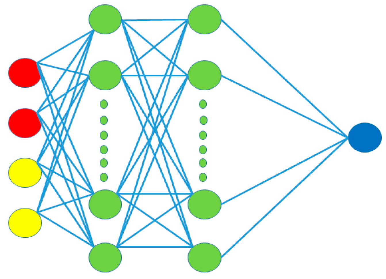
In DQN, if the state space is represented as a set of feature values (e.g., speed, acceleration, etc.), the network typically employs a fully connected architecture, also known as a feedforward neural network, which is shown in Figure 6. This network consists of an input layer, hidden layers, and an output layer, with each neuron in a layer fully connected to the neurons in the subsequent layer.

The neural network architecture used in this study consists of four layers, implemented as follows:

The input layer applies a linear transformation to the state vector s using a weight matrix W1 of shape [s,200] and a bias vector b1 of shape [1,200], followed by a ReLU activation function. The output of this layer is denoted as layer1.

The second hidden layer consists of 100 neurons. It receives the output from the first layer and applies a linear transformation with weight matrix W2 of shape [200,100], and bias vector b2 of shape [1,100], followed by a ReLU activation.

The third hidden layer, consisting of 50 neurons, receives the output from the second layer. A linear transformation is applied using weight matrix W3 of shape [100,50] and bias vector b3 of shape [1,50], followed by a ReLU activation.

The output layer computes the final Q-value estimation. A linear transformation is applied to the output from the third layer using weight matrix W4 of shape [50,1] and bias vector b4 of shape [1,1].

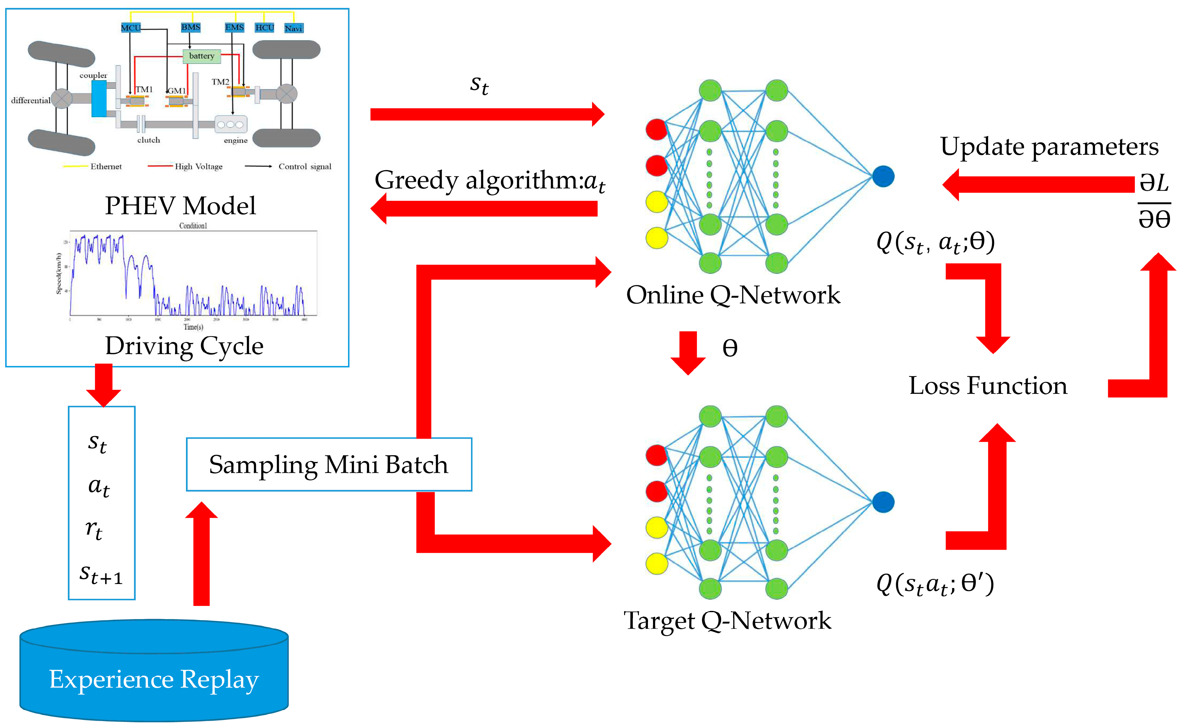
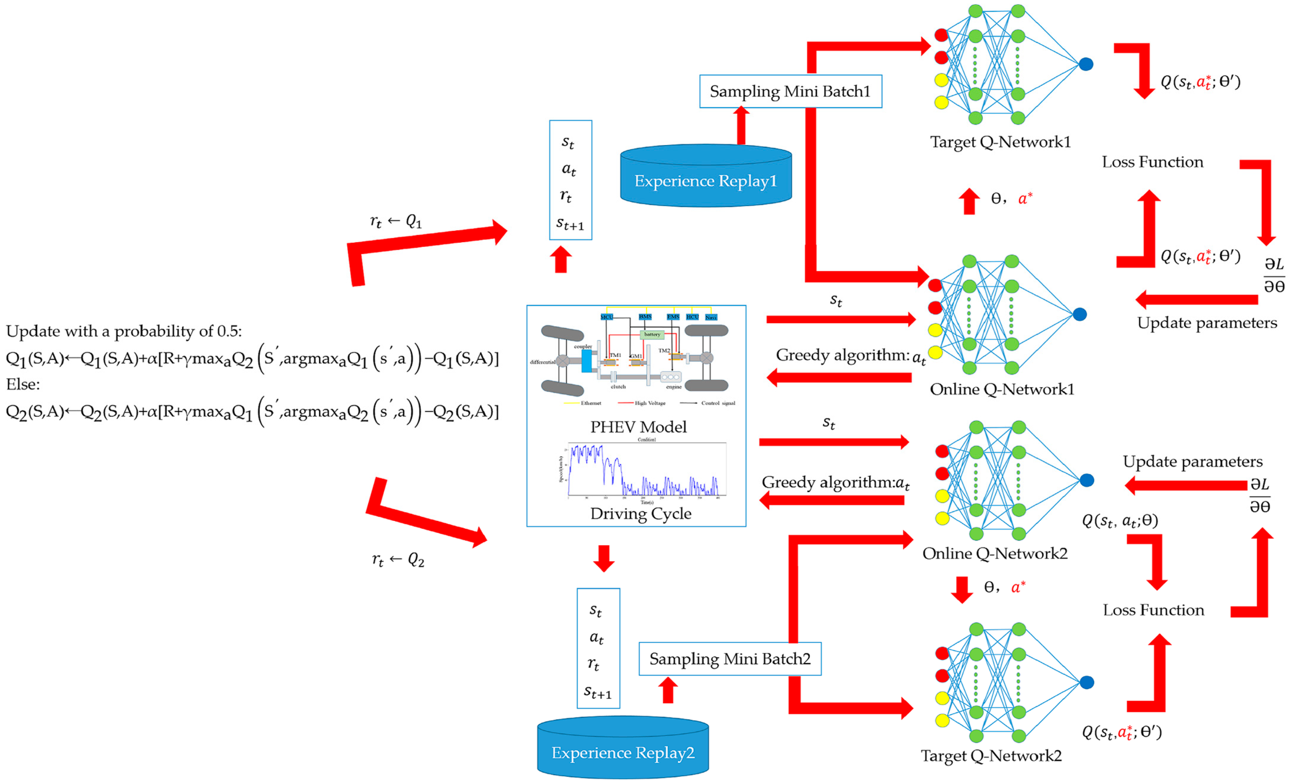
In this approach, two Q-networks are employed. As shown in Figure 7, the first network, the Online Q-Network, interacts with the environment by taking the state vector (v, a, SOC) as input and producing the optimal action a_t based on the Q-value ranking. The second network, the Target Q-Network, calculates the target Q-value for the given state vector input. Additionally, an Experience Replay buffer is utilized to store previously collected data, which are then sampled and fed into both Q-networks to optimize their parameters.

In reinforcement learning, the agent’s sequential decision-making process often results in highly correlated data, which can destabilize convergence, particularly when using complex function approximators like neural networks. Experience Replay addresses this by randomly sampling past experiences to produce training data that are more independent and identically distributed, thus reducing the temporal correlation’s impact on the learning process. By balancing sampling from the buffer, Experience Replay reduces sensitivity to random or extreme values, smoothing the training process and minimizing the variance in network updates. A loss function is designed to optimize the Q-network parameters by minimizing the RMS error between the two Q-values.

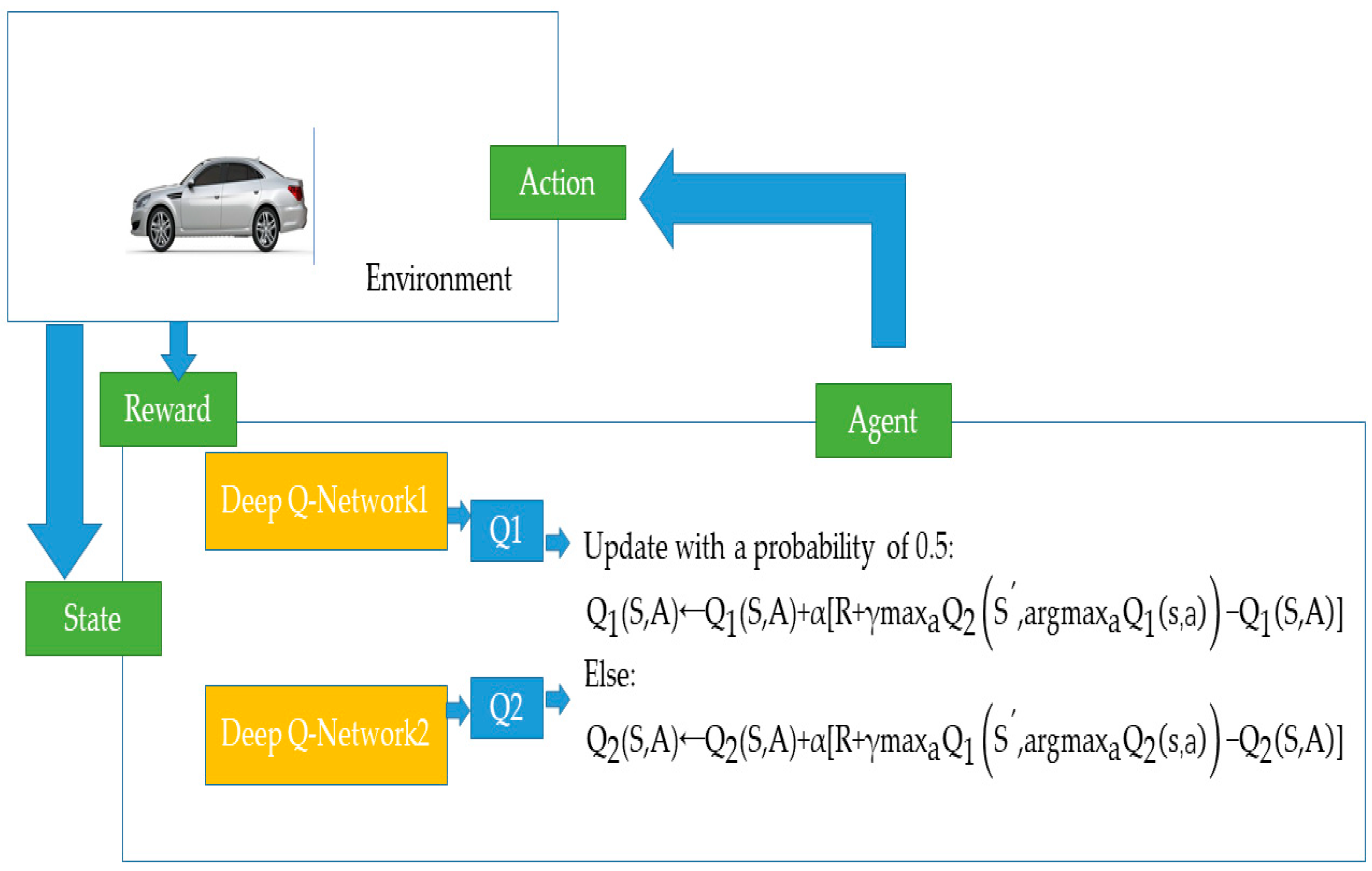
3.3. Double Deep Q-Network

Based on the description in Sutton’s book [28], control algorithms built upon goal-maximizing policies, such as Q-learning, rely on a greedy policy with respect to the current action-value. In this algorithm, the target policy implicitly uses the maximum estimated value as a proxy for the actual maximum, leading to maximization bias. Specifically, for a single state s, the true value q(s,a) for each action a is zero, but its estimate Q(s,a) is uncertain and distributed around zero. Consequently, while the true maximum value is zero, the estimated maximum is positive, introducing a maximization bias.

In the scenario of vehicle energy management, a similar problem arises. Here, uncertainties in vehicle speed, acceleration, and SOC lead to unpredictable states, and uncertainties in the applied actions (engine and motor torque) contribute to maximization bias. This bias results in inaccurate Q-value estimation, which prolongs the computation time required to identify the optimal action. To mitigate this issue, we propose using identical samples to both determine the maximizing action and estimate its value. This approach involves partitioning the vehicle’s operating data into two sets, which are used to independently estimate two separate Q-values, denoted as Q1(a) and Q2(a) for $\mathrm{a}\in \mathrm{A}$, both of which approximate the true value q(a).

The roles of Q1 and Q2 can be reversed in subsequent iterations: Q2 can identify the action, while Q1 estimates the value. This step process allows for alternated updates between Q1 and Q2, with each producing optimal actions, a technique termed the Double Deep Q-Network (DDQN) in Figure 8.

Update with a probability of 0.5:

$${\mathrm{Q}}_1(\mathrm{S},\mathrm{A})\leftarrow {\mathrm{Q}}_1(\mathrm{S},\mathrm{A})+\alpha [\mathrm{R}+\gamma {\max }_{\mathrm{a}}{\mathrm{Q}}_2\left({\mathrm{S}}^{\prime },\arg {\max }_{\mathrm{a}}{\mathrm{Q}}_1\left(\mathrm{s},\mathrm{a}\right)\right)-{\mathrm{Q}}_1\left(\mathrm{S},\mathrm{A}\right)]$$

(9)

Else:

$${\mathrm{Q}}_2(\mathrm{S},\mathrm{A})\leftarrow {\mathrm{Q}}_2(\mathrm{S},\mathrm{A})+\alpha [\mathrm{R}+\gamma {\max }_{\mathrm{a}}{\mathrm{Q}}_1\left({\mathrm{S}}^{\prime },\arg {\max }_{\mathrm{a}}{\mathrm{Q}}_2\left(\mathrm{s},\mathrm{a}\right)\right)-{\mathrm{Q}}_2\left(\mathrm{S},\mathrm{A}\right)]$$

(10)

The pseudocode of the DDQN-based EMS in offline training is listed in Algorithm 1.

Algorithm 1. Pseudocode of the DDQN-based EMS.

1 Initialization: experience pool of DQN1 and DQN2 with capacity N = 10,000; 2 Randomly initialize the parameters of online and target network; 3 for each episode do: 4  Observe initial state 5   for t = 1 to end do: 6   control engine throttle a* = argmaxa∈AQ(s,a|ϴ)(1−ε)probability or randomly output action ε probability 7    PHEV return performs actions and return reward and next state 8    ${\mathrm{Q}}_1(\mathrm{S},\mathrm{A})\leftarrow {\mathrm{Q}}_1(\mathrm{S},\mathrm{A})+\alpha [\mathrm{R}+\gamma {\max }_{\mathrm{a}}{\mathrm{Q}}_2\left({\mathrm{S}}^{\prime },\arg {\max }_{\mathrm{a}}{\mathrm{Q}}_1\left(\mathrm{s},\mathrm{a}\right)\right)-{\mathrm{Q}}_1\left(\mathrm{S},\mathrm{A}\right)]$ with 0.5 probability $\mathrm{or}\hspace{1em}\hspace{1em}\hspace{1em}\hspace{1em}{\mathrm{Q}}_2(\mathrm{S},\mathrm{A})\leftarrow {\mathrm{Q}}_2(\mathrm{S},\mathrm{A})+\alpha [\mathrm{R}+\gamma {\max }_{\mathrm{a}}{\mathrm{Q}}_1\left({\mathrm{S}}^{\prime },\arg {\max }_{\mathrm{a}}{\mathrm{Q}}_2\left(\mathrm{s},\mathrm{a}\right)\right)-{\mathrm{Q}}_2\left(\mathrm{S},\mathrm{A}\right)]$ 9    store sampling [st,at,rt,st+1] 10     select mini batch size samples from the experience pool 11     update the weights of each Online Q-Network and copy the parameters from online Q to target Q after several training episodes 12     end for 13  end for

4. Quadruple Deep Q-Network

As shown in Equations (11)–(13), the action A* that maximizes Q1 is identified, while Q2 provides an unbiased estimate of its value. Unlike the previous method, where the target Q-value is selected as the maximum Q-value from the Target Q-Network, the approach here selects the action A* that maximizes the Q-value from the Online Q-Network. Then, in the Target Q-Network, the corresponding Q-value for the next state S’ is chosen as the target Q-value. After updating both Q1 and Q2 networks using this approach, the Q-values are further updated in a cross-update fashion to mitigate the previously mentioned maximization bias issue. This framework is shown in Figure 9.

$${\mathrm{A}}^{*}=\arg {\max }_{\mathrm{a}}{\mathrm{Q}}_1\left(\mathrm{a}\right)$$

(11)

$${\mathrm{Q}}_2\left({\mathrm{A}}^{*}\right)={\mathrm{Q}}_2(\arg {\max }_{\mathrm{a}}{\mathrm{Q}}_1\left(\mathrm{a}\right))$$

(12)

$$\mathrm{E}\left|{\mathrm{Q}}_2\left({\mathrm{A}}^{*}\right)\right|=\mathrm{q}\left({\mathrm{A}}^{*}\right)$$

(13)

5. Validation and Discussion

5.1. Comparison of Different DQN Methods

Here, the hyperparameters were selected as shown in

Table 2. Main component parameters of PHEV.

Hyperparameters	Values
Mini-batch size	32
Experience pool size	10,000
Discount factor	0.9
Learning rate	0.9
Target network update frequency	10

. In practice, however, different learning rates and discount factors can significantly impact the final performance, specifically affecting the Q-value estimates, the SOC curve progression, and fuel consumption, so we can change them to see the results.

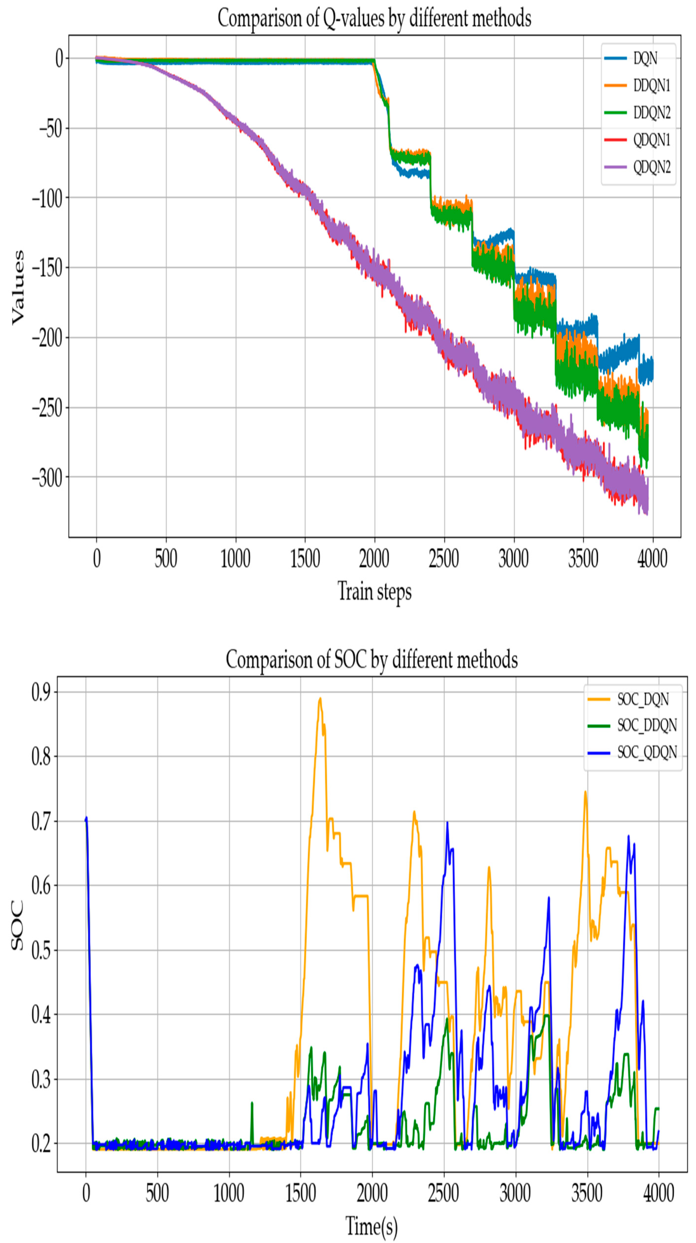
As shown in Figure 10, the initial SOC is set to 0.7. After 100 episodes of training, with a learning rate α = 0.9, discount rate γ = 0.9, and greedy factor ε = 0.1, we can observe the changes in Q-values. For the DQN, the initial Q-value is zero and does not begin to update until after around 2000 steps, indicating that the true Q-value, a negative value with an absolute magnitude of up to 350, is reached relatively slowly. In comparison, the Q-value updates in the two Q-networks of the DDQN are also not significantly accelerated, likely due to the 0.5 probability of randomly selecting a Q-network, resulting in each network being updated only half as frequently within each 10-episode interval. The QDQN, however, updates more rapidly, beginning to decrease after only 500 steps. This result demonstrates the advantage of the proposed QDQN in accelerating Q-value convergence, indicating that it can achieve the optimal solution more quickly within the same number of episodes.

Next, we can observe the SOC change curve. Under the same penalty function, the DQN method allows the SOC to charge up to 0.9, which could lead to battery overcharging in practical scenarios. In contrast, the SOC variations with DDQN are more gradual. After an initial discharge from 0.7, DDQN initiates moderate recharging at 1000 s. Comparing these timings to the speed-time curve, the initial speed is 120 km/h, decreasing to 80 km/h at 1000 s and 30 km/h at 1500 s. Additionally, DDQN performs recharging more effectively than DQN, maintaining the SOC around 0.35, which prevents overcharging and contributes to further energy savings. The SOC curve of QDQN falls between the two others.

Use Equation (14) to calculate total energy consumption under different operating conditions, where E_equivalent denotes total energy consumption, E_fuel denotes fuel consumption, PH is the energy density of fuel, set at 44 MJ/kg, and E_bat denotes the energy consumed by the battery.

E_equivalent = E_fuel × PH + E_bat

(14)

As shown in

Table 3. Results of Different EMSs in the training process with α = 0.9, γ = 0.9, ε = 0.1.

Method	Initial SOC	Final SOC	Fuel_100 km	Equivalent Energy	Gap
DQN	0.7	0.199	2.107 kg	192.65 MJ	-
DDQN	0.7	0.253	1.334 kg	129.9 MJ	32.9%
QDQN	0.7	0.218	1.704 kg	160.5 MJ	16.7%

, the equivalent energy consumption for the three strategies is 192.65 MJ, 129.9 MJ, and 160.5 MJ, respectively. It can be concluded that updating the Q-values with a probability of 0.5 results in a 32.9% increase in energy consumption. On the other hand, using the QDQN algorithm leads to a 16.7% increase in energy consumption.

The slightly inferior performance of QDQN compared with DDQN can be attributed to the incorporation of A* into the target network. This approach introduces a more aggressive update mechanism, which can lead to instability in the learning process. Therefore, it is advisable to adopt a more cautious strategy when updating Q-values and selecting actions to avoid excessive overestimation and ensure more stable learning dynamics.

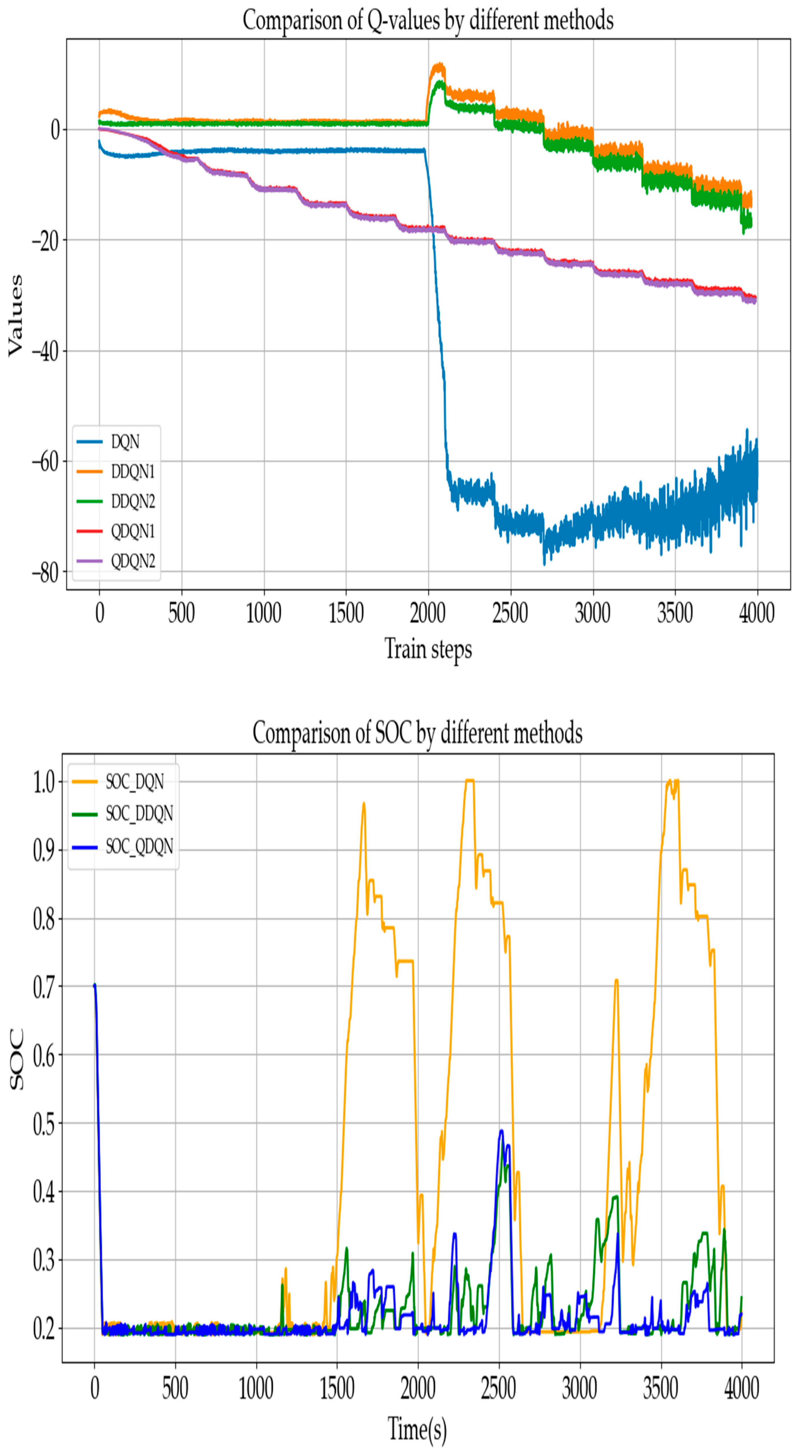
In the second experiment, as shown in Figure 11, a training scenario with a learning rate of α = 0.5 and a discount factor of γ = 0.5 greedy factor ε = 0.1 is examined. Initially, for the Q-values, the QDQN begins to converge towards the true values after approximately 500 steps, while the DQN remains unchanged at zero. The Q-values of the DDQN, on the other hand, show no decline. By step 2000, the DDQN continues to exhibit an upward trend, indicating that relying solely on alternating updates of the two Q-networks has limited effectiveness. At this point, the QDQN has steadily decreased to −40, suggesting that action alternation should be incorporated into the Q-value update process. Meanwhile, the DQN experiences a sharp drop to −70 at step 2000, followed by a recovery to −60, indicating the presence of overestimation. The QDQN, however, better addresses this issue, as it not only decreases steadily but also avoids sudden rebounds, demonstrating superior estimation characteristics.

By observing the SOC curve, it can be seen that during the high-speed phase, all three algorithms effectively utilize the battery energy, with the SOC decreasing from around 0.7 to approximately 0.2. Around 1500 s, when the vehicle speed decreases and under consistent penalty functions, the DQN begins to recharge, while the DDQN also increases the SOC from 0.2 to above 0.4. Both algorithms exhibit significant charging behavior during driving. In contrast, the QDQN maintains the SOC between 0.2 and 0.5 around 2500 s. This indicates that the variations in learning rate, discount factor, and greedy factor have an impact on the algorithms, while they significantly affect the DQN and DDQN, further confirming the stronger robustness of QDQN.

Finally, by observing the overall energy consumption in

Table 4. Results of Different EMSs in the training process with α = 0.5, γ = 0.5, ε = 0.1.

Method	Initial SOC	Final SOC	Fuel_100 km	Equivalent Energy	Gap
DQN	0.7	0.223	1.972 kg	182.26 MJ	-
DDQN	0.7	0.205	1.448 kg	141.6 MJ	22.5%
QDQN	0.7	0.191	1.137 kg	117.9 MJ	35.7%

, it is evident that all of the algorithms show a significant increase in fuel consumption per 100 km when the learning rate and discount factor are set to lower values. This suggests that improving the update frequency yields better performance. However, the QDQN shows max increase. From the perspective of total energy consumption, the DQN consumes 182.26 MJ, and the DDQN consumes 141.6 MJ, while the QDQN consumes 117.9 MJ. The QDQN and DDQN exhibit a 35.7% and 22.5% energy saving, respectively, compared with the DQN, demonstrating a significant improvement in efficiency.

5.2. Comparison Between DQN Methods and DP

The problem of fuel consumption during vehicle operation is modeled as a Markov Decision Process (MDP), with the core focus being the solution of the Bellman equation:

$${\mathrm{V}}^{*}\left(\mathrm{s}\right)=\underset{\pi }{\max }{\sum }_{\mathrm{a}}\pi \left(\mathrm{a}|\mathrm{s}\right)[\mathrm{r}+\gamma {\mathrm{V}}^{*}\left({\mathrm{s}}^{\prime }\right)]$$

(15)

${\mathrm{V}}^{*}\left(\mathrm{s}\right)$ represents the expected value function of current state, ${\mathrm{V}}^{*}\left({\mathrm{s}}^{\prime }\right)$ represents the next state’s value function, $\pi \left(\mathrm{a}|\mathrm{s}\right)$ represents the probability of selecting action a in state s. Through iterative updates, the method aims to select the optimal action.

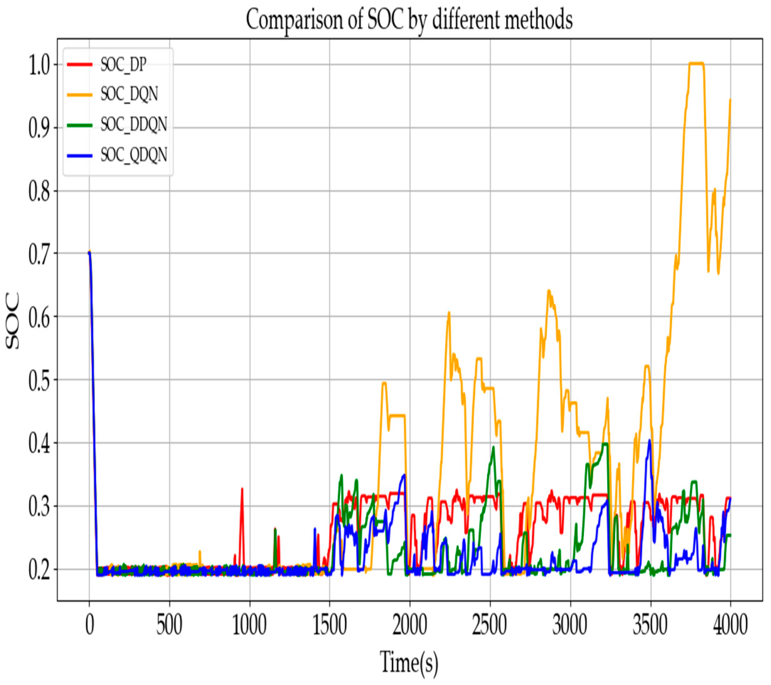
In the final set of experiments, shown in Figure 12 and

Table 5. Results of Different EMSs in the training process with α = 0.9, γ = 0.9, ε = 0.001.

Method	Initial SOC	Final SOC	Fuel_100 km	Equivalent Energy	Gap
DP	0.7	0.329	1.361 kg	127.24 MJ	-
DQN	0.7	0.942	1.838 kg	126.8 MJ	0.78%
DDQN	0.7	0.253	1.234 kg	122.2 MJ	3.9%
QDQN	0.7	0.31	1.166 kg	113.5 MJ	11.0%

, with the parameter settings of α = 0.9, γ = 0.9, and ε = 0.001, it is evident that the learning rate and discount factor primarily influence the variation in SOC. The exploration–exploitation rate ε significantly impacts action selection, which in turn affects energy consumption. A smaller ε-value leads to better results, as it helps avoid local optima in the action selection process. In comparison with DP, the proposed QDQN achieves an 11% improvement in energy efficiency. As shown by the SOC curve, QDQN results in fewer charging cycles and, with the same number of training episodes, QDQN is able to identify a more optimal solution.

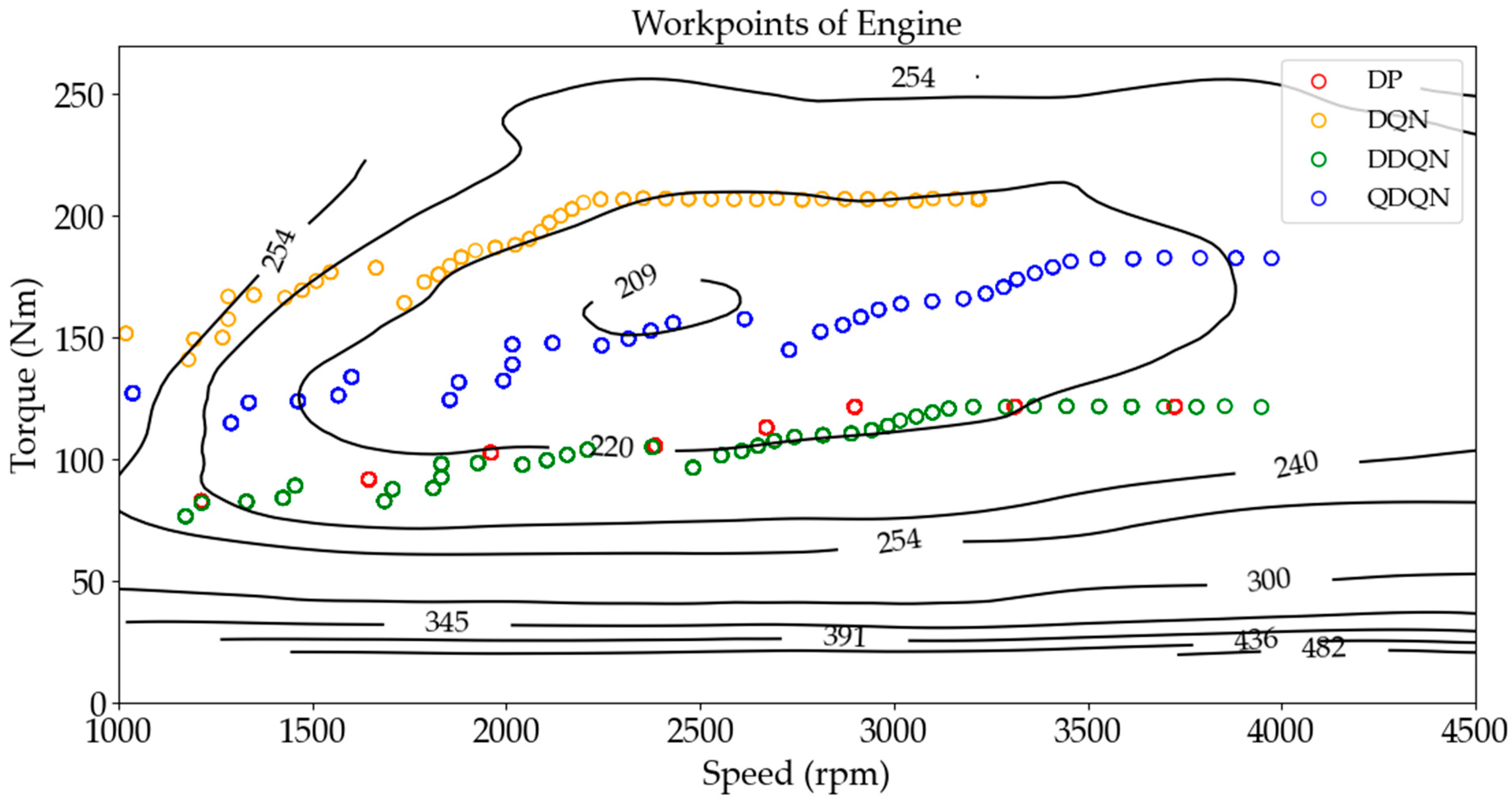
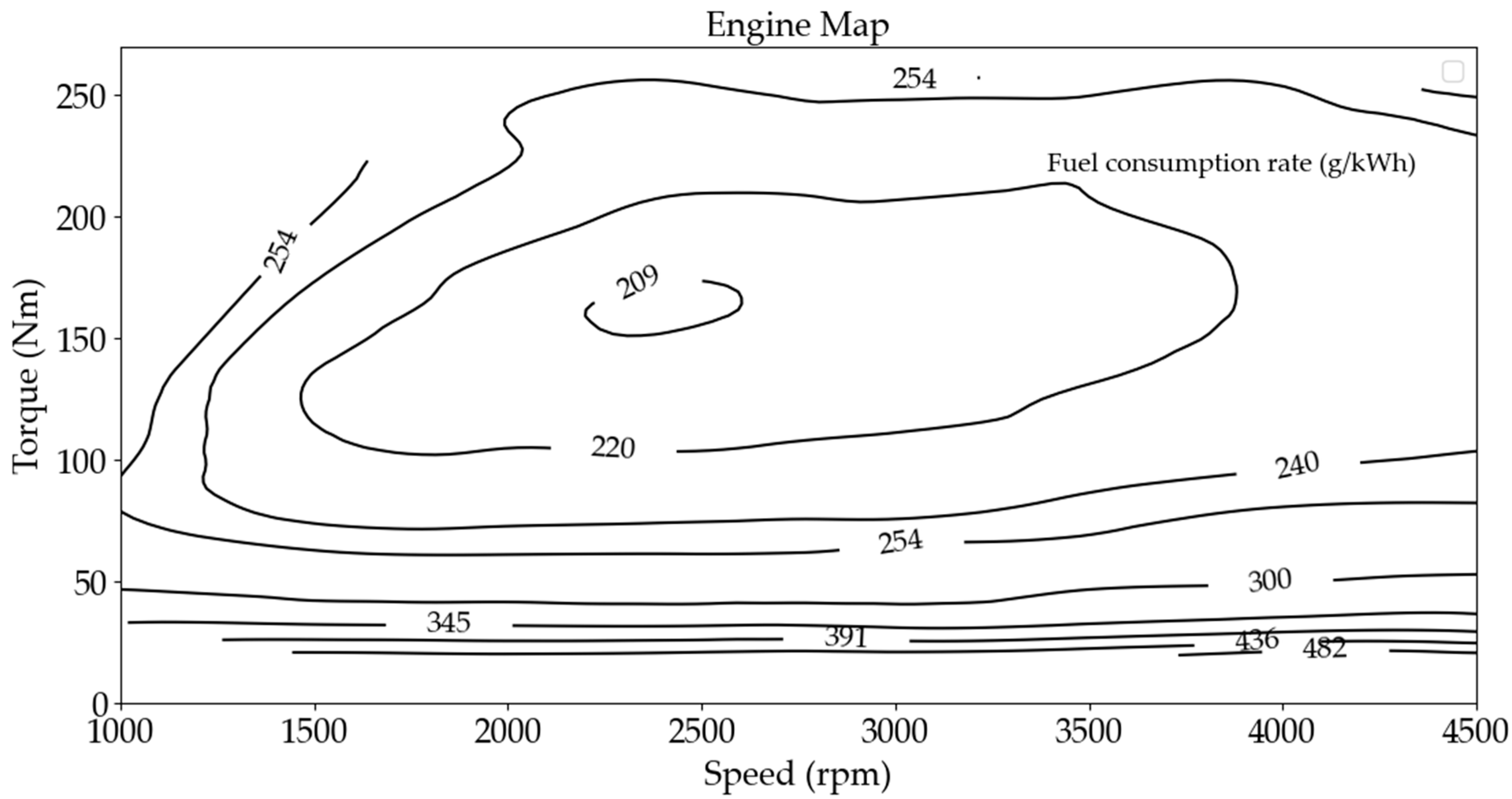
As shown in Figure 13, the distribution of engine operating points under various algorithms is depicted. It can be observed that all these algorithms generate a series of points, which are relatively concentrated rather than scattered. First, the operating points of these algorithms are discrete. Due to computational limitations, DP exhibits a more scattered distribution. In contrast, other deep learning-based algorithms can select a larger set of operating points. DQN converges more slowly, resulting in a concentration of operating points in the high-torque region. While DDQN’s operating points overlap with those of DP, it benefits from improved computational performance, allowing for a greater selection of points and reducing computation time. QDQN accelerates the iteration process, resulting in operating points that are more concentrated in the low fuel consumption region.

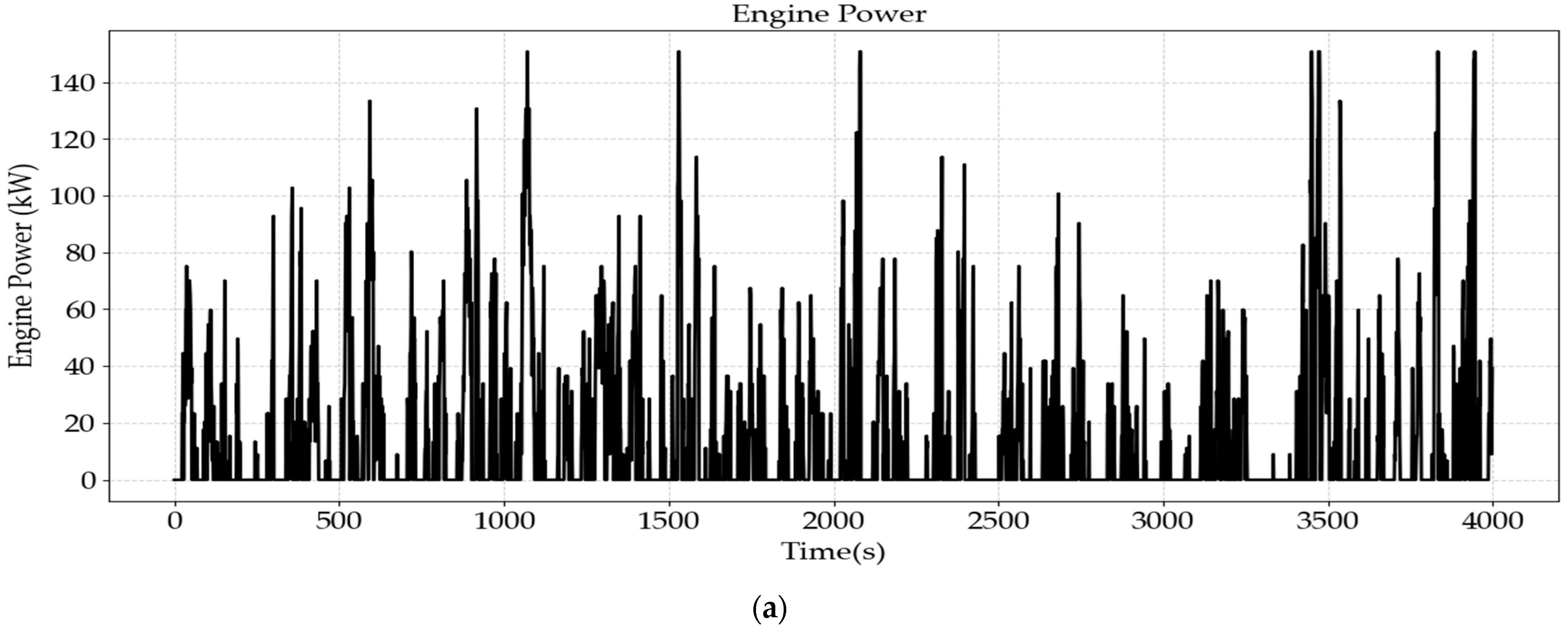
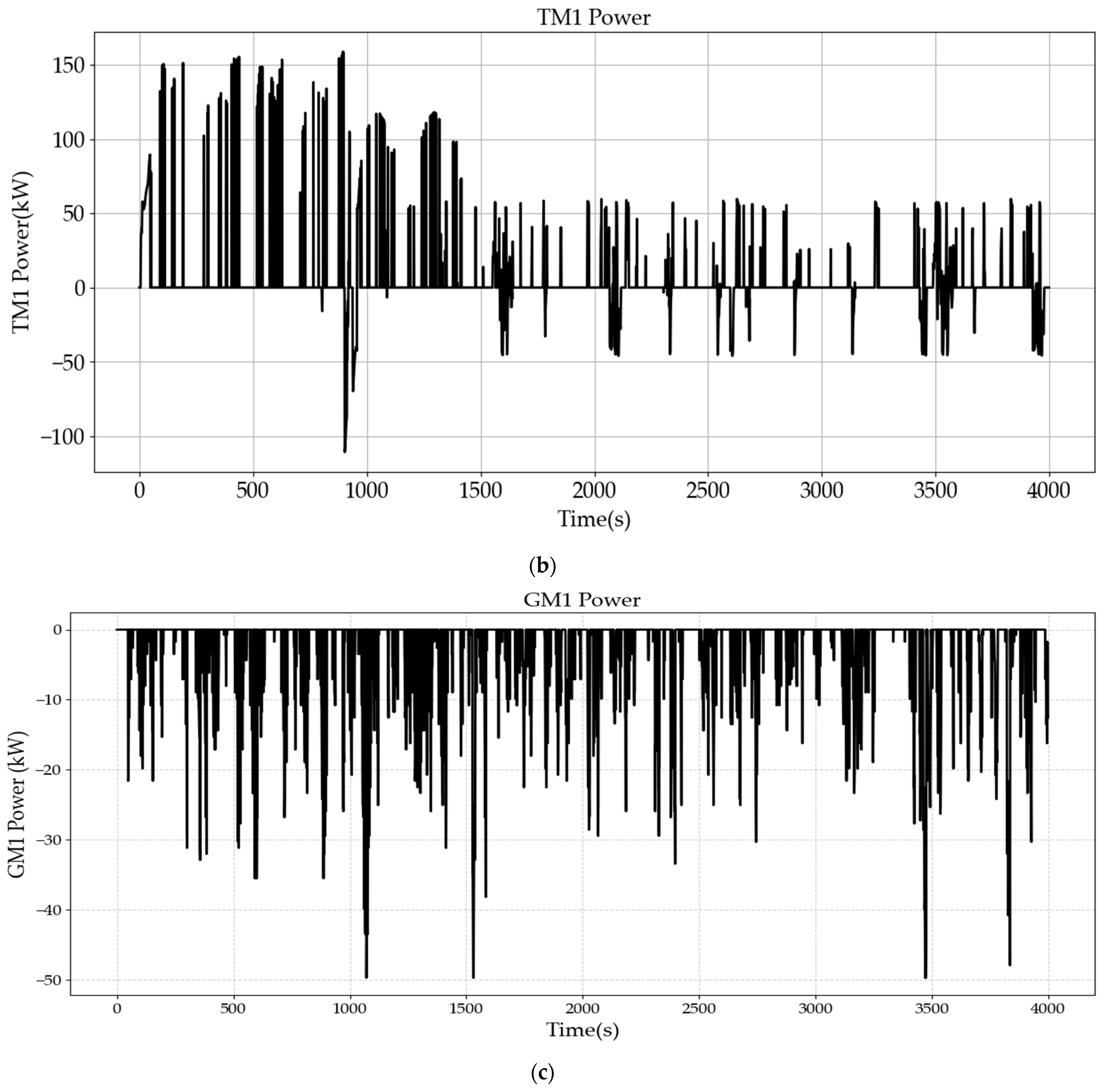
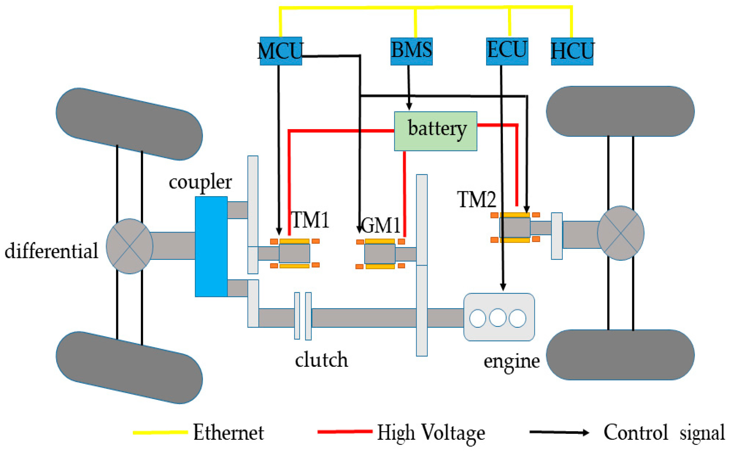
Based on Figure 14, the energy flow under the application of the QDQN algorithm can be analyzed. During the time period of 0–1000 s, the vehicle operates at high speed. Both the engine and the battery exhibit significant power output to meet the high power demand. Simultaneously, the generator operates with considerable power output for electricity generation. The driving power of TM1 and TM2 is jointly supplied by the engine and the battery.

Between 1000 and 1500 s, the vehicle speed decreases slightly, entering a medium-speed range. A portion of the engine’s output is allocated for electricity generation, while the battery’s power output decreases slightly. Consequently, the power output of TM1 and TM2 also shows a decline.

After 1500 s, the average power demand drops significantly. To maintain the state of charge (SOC) above 0.2, a portion of the engine’s power continues to be used for electricity generation, and the power output of TM1 and TM2 further decreases.

Overall, the trends in power output of each powertrain component align with the variations in vehicle speed. This indicates that the QDQN algorithm effectively optimizes energy management through training.

5.3. Feasibility of Real-World Implementation

Each time the vehicle state changes, a quick decision must be made, which requires the deep neural network (FNN) to perform forward propagation within a short period. QDQN includes both a policy network and a target network, which need to be updated alternately while handling large state spaces and complex models. Therefore, real-time QDQN inference, typically in the millisecond range, demands a processor with a high clock frequency. Processors with a frequency range of 1.5–2.5 GHz are commonly found in modern onboard hardware and can support such computations. Batch updates require processing tens to hundreds of samples, which increases the computational load. A QDQN model generally requires between 50–200 MB of memory, depending on the complexity of the network. Onboard systems should reserve additional space for system operations, input and output data, and logs, suggesting a total memory requirement of 1–2 GB.

Simpler RL-based algorithms, such as DP, have higher storage and computational requirements. For instance, DP requires calculating various allocation scenarios for each speed point and then comparing them to determine the minimum energy consumption and corresponding actions. This process is more resource-intensive in terms of both time and space.

In summary, QDQN is feasible for onboard implementation in modern PHEVs equipped with advanced automotive processors. The computational requirements are manageable within the capabilities of contemporary hardware, ensuring that the advantages of QDQN in energy optimization outweigh the additional hardware demands.

6. Conclusions

In this study, the QDQN algorithm is proposed to optimize the energy management strategy for PHEVs. Compared with the energy management strategies based on DP, DQN, and DDQN, with appropriate selections of learning rate, discount factor, and exploration–exploitation strategy, the QDQN-based strategy achieves improvements in energy efficiency utilization by up to 11%, 10.2%, and 7.1%, respectively. Additionally, this study confirms another key finding: alternating updates between the two networks can significantly enhance energy efficiency utilization. This approach yields even better results, particularly when the greedy strategy in the current network becomes trapped in a local optimum.