Article

Substation Abnormal Scene Recognition Based on Two-Stage Contrastive Learning

1
State Grid Henan Electric Power Research Institute, Zhengzhou 450199, China
2
State Grid Henan Electric Power Company, Zhengzhou 450052, China
3
School of Artificial Intelligence, Anhui University, 111 Jiulong Road, Hefei 230601, China
*
Author to whom correspondence should be addressed.
Energies 2024, 17(24), 6282; https://doi.org/10.3390/en17246282
Submission received: 12 October 2024 / Revised: 9 December 2024 / Accepted: 10 December 2024 / Published: 13 December 2024
(This article belongs to the Special Issue Energy, Electrical and Power Engineering: 3rd Edition)

Abstract

:
Substations are an important part of the power system, and the classification of abnormal substation scenes needs to be comprehensive and reliable. The abnormal scenes include multiple workpieces such as the main transformer body, insulators, dials, box doors, etc. In this research field, the scarcity of abnormal scene data in substations poses a significant challenge. To address this, we propose a few-show learning algorithm based on two-stage contrastive learning. In the first stage of model training, global and local contrastive learning losses are introduced, and images are transformed through extensive data augmentation to build a pre-trained model. On the basis of the built pre-trained model, the model is fine-tuned based on the contrast and classification losses of image pairs to identify the abnormal scene of the substation. By collecting abnormal substation images in real scenes, we create a few-shot learning dataset for abnormal substation scenes. Experimental results on the dataset demonstrate that our proposed method outperforms State-of-the-Art few-shot learning algorithms in classification accuracy.

1. Introduction

Substations are an indispensable part of the power system, and their normal operation is crucial for the stability and safety of the power system [1]. However, substation equipment is usually exposed to the open environment and is subject to natural weather conditions, leading to issues such as rust, aging, and component detachment. Additionally, staff non-compliance with operational standards and disturbances from the natural environment, such as bird nests on transformers, are common occurrences. These abnormal situations pose potential threats to the operational safety of substations, necessitating timely detection and identification of abnormal scenarios within substations. With the continuous expansion of substation scales, traditional manual inspection methods for power inspection tasks are facing challenges, the most significant of which is the low efficiency and susceptibility to environmental influences. Moreover, manual inspections are also limited by subjective judgments [2]. The subjective judgment of inspectors can be easily influenced by various factors, such as fatigue, visual limitations, and personal biases, thereby increasing potential safety risks. Ensuring the safe inspection of substation systems has become an important issue that needs to be addressed urgently. Given the limitations of traditional manual inspection methods, there is an urgent need to introduce new technologies and methods to improve inspection efficiency and accuracy.
Currently, substation equipment can be inspected by using inspection robots to collect images on-site, followed by applying machine learning algorithms for abnormal scenario recognition. Kong et al. [3] were the first to apply pattern recognition technology for the video monitoring of unattended substations, using the AdaBoost algorithm for weighted voting to detect moving targets, successfully achieving recognition of abnormal environments. Wu et al. [4] introduced the concept of a fault detection algorithm based on improved YOLO5 that sets a hyperparameter at each layer according to the recognition situation to re-extract features for substation equipment. Gao et al. [5] combined YOLOX with higher-order gated convolution to enhance the interaction capability in feature space, improving detection accuracy and robustness. However, the number of images for abnormal scenarios in substations is relatively small, resulting in an imbalance between positive and negative samples. Researchers have proposed innovative solutions for this issue, such as augmenting the training set with virtual abnormal samples generated using generative adversarial networks [6] to achieve a numerical balance between positive and negative samples. Additionally, techniques like transfer learning and semi-supervised learning can be employed to train with a few labeled abnormal samples [7]. However, the field primarily faces two challenges: (1) a large number of abnormal scenario categories with significant differences between each scenario and (2) the difficulty in collecting abnormal scenario samples, resulting in a limited number of samples. In fact, abnormal scenario recognition in substations is a typical few-shot learning problem. The backgrounds and objects to be identified in different abnormal situations exhibit distinct differences, which leads to poor generalization capabilities of existing models and difficulties in accurately identifying new abnormal scenarios.
Numerous scholars have conducted related research to address the challenges of machine learning in substation abnormal scene recognition with small sample sizes. In the field of few-shot learning, the researchers divided the dataset into a base set and a support set. The base set is used to train a foundational model with a limited number of labeled samples, and the support set is employed to evaluate and further fine-tune the model’s performance. The support set consists of a small number of support samples and query samples; support samples are used for model evaluation, and query samples are utilized for performance measurement. Small-sample models aim to classify query samples using support samples. To cope with few-shot learning scenarios, metric learning methods [8,9] are widely used to learn the feature space of samples in the base set, which is then applied to classify query samples in the support set. However, when recognizing abnormal scenes in substations, these methods face challenges due to the large differences in sample morphology, the scarcity of samples for certain defects, and large numbers of unlabeled samples. Therefore, some researchers have adopted self-supervised learning to perform the task. Usually, they use data augmentation on the base dataset to construct a pre-trained model and then fine-tune the pre-trained model with the support set to build a classifier. Nevertheless, existing algorithms neglect the distinctiveness and diversity among samples when handling abnormal scene samples in substations, resulting in poor classification performance. The abnormal scenarios in substations significantly differ in sample morphology, with specific categories of defects encompassing very few samples, and many samples are without annotated labels. Constructing a model that correctly identifies each defective instance under small-sample conditions poses a significant challenge. Inspired by self-supervised learning, this paper proposes a novel two-stage contrastive learning (2-SCL) method for identifying abnormal scenes in substations. It combines contrastive learning with various data augmentation techniques in the first stage to construct a pre-trained model, aiming to minimize the distance between original and augmented samples, thereby enhancing sample distinctiveness and improving the model’s inter-class discrimination and generalization ability. At the same time, to prevent the distance between similar samples from becoming too far, this paper proposes supervised contrastive learning for fine-tuning to further improve performance, effectively addressing the problems existing research in this field faces.
To implement self-supervised tasks, it is necessary to perform data augmentation on the original image [10]. In fact, data augmentation of samples is crucial for improving the algorithm’s performance. In the proposed algorithm, various complex transformations are used to generate multiple transformations and utilize self-supervised objectives to learn rich representations, thereby enabling the model to have better discrimination for different category samples. Furthermore, based on the pre-trained model, the support set enables the learned model to use fewer samples and classify query samples more accurately. The main contributions of this paper are as follows:
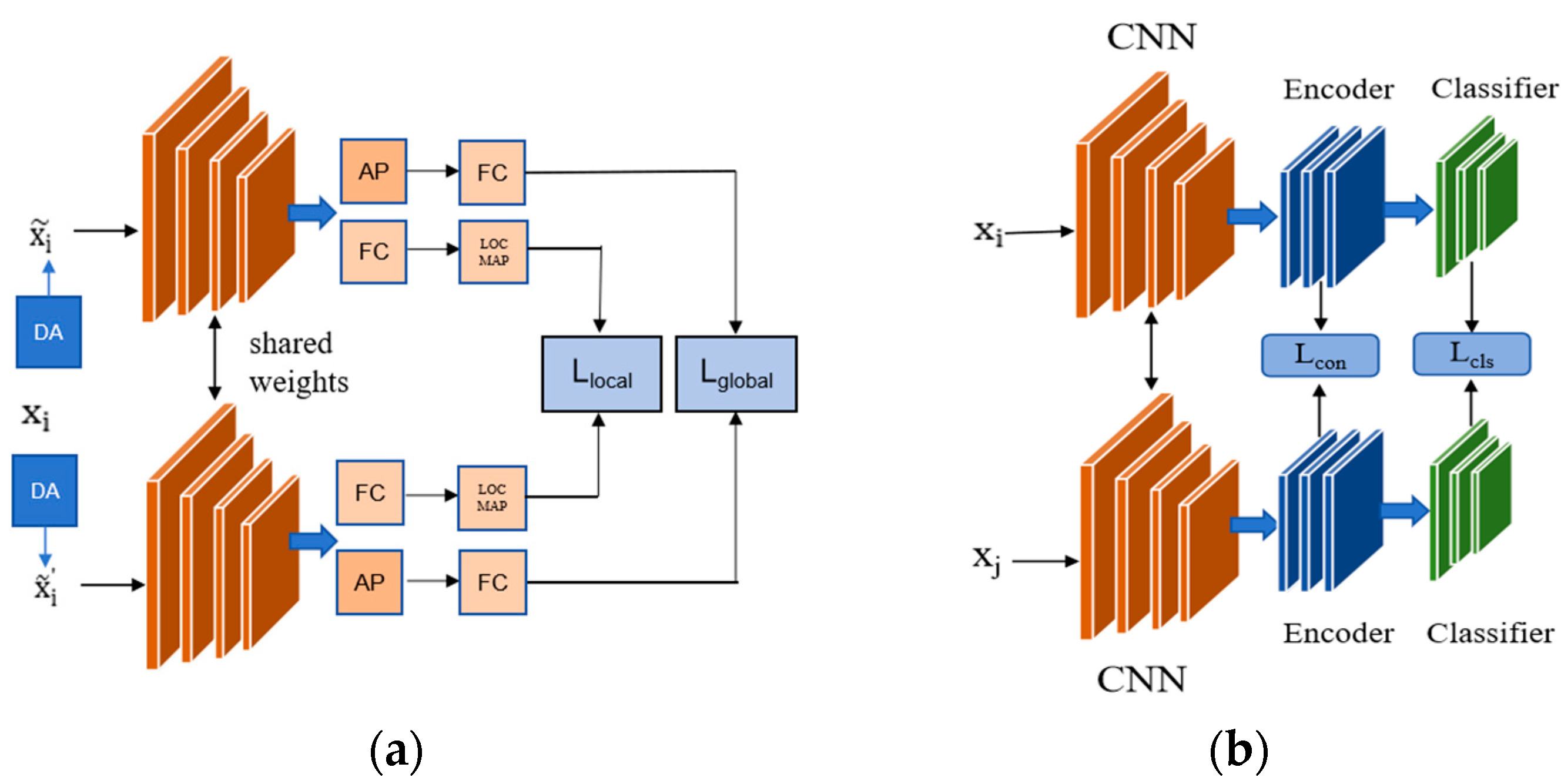
  • A novel few-shot learning method, which utilizes two-stage contrastive learning (2-SCL) to construct the learning objective, is proposed. In the first stage, a pre-trained model is constructed through self-supervised learning, thereby enhancing the model’s inter-class discrimination ability.
  • Supervised contrastive learning is introduced in the second stage of the model, further fine-tuning the pre-trained model within a supervised framework to improve sample identification capability and model generalization ability.
  • In the self-supervised phase, multiple data augmentation methods are proposed to enhance sample diversity, thereby obtaining more generalized feature representations.
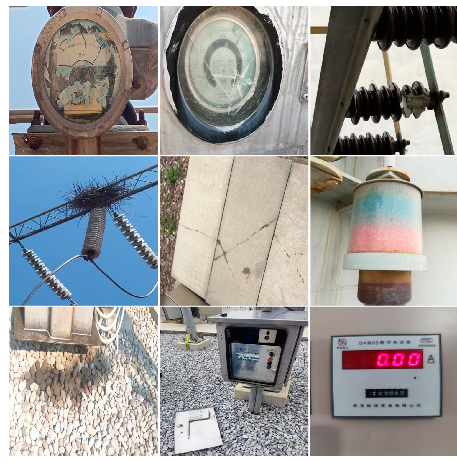
  • A large-scale dataset of substation abnormal scenarios has been constructed, which can provide better data support for subsequent research.

2. Related Work

This section introduces some existing work on small-sample learning and self-supervised learning algorithms.

2.1. Few-Shot Learning

The primary objective of few-shot learning is to train a model that can classify the samples of unseen classes with limited training samples. Many researchers have proposed methods based on metric learning to address the few-shot learning problem. Early studies utilized Siamese neural networks [11] to recognize the similarity between support and query samples through the L1 distance (The distance measures the sum of the absolute differences between the coordinates of the feature vector). MatchingNet [12] employed different networks to extract features from support and query samples and calculated their similarity using cosine distance. In recent years, attention mechanisms have also been widely applied to few-shot learning. For instance, Ref. [13] introduced a cross-attention module to improve detection performance by capturing the accurate target area, while the self-attention mechanism [14] was used to explore task-specific information. Moreover, building a pre-trained model on a large dataset without class labels and then fine-tuning it on small-sample data [15] has been proven effective in enhancing recognition performance. RelationNets [16] first uses a Relation Network (RN) that learns an embedding and a deep non-linear distance metric for comparing query and sample items through end-to-end and episodic training. In contrast, RelationNets2 [17] learns multiple non-linear distance metrics for few-shot learning and achieves State-of-the-Art results. A prototypical network [18] is proposed for few-shot and zero-shot learning, which learns a metric space by computing distances to prototypes, achieving excellent results with a simpler design. Ref. [19] uses ridge regression as the main adaptation mechanism for few-shot learning to enable deep networks to quickly adapt to novel data, achieving competitive performance.

2.2. Self-Supervised Learning

Self-supervised learning is a method that constructs a pre-trained model in a supervised manner by introducing self-supervised objectives. Early studies [20] used a set of image-augmented samples to predict categories; while ref. [21] employed the model to predict the rotation angle of images to better extract features and improve classification performance. Self-supervised learning [22] has also been used to predict the position of patches after random cropping of images, thus enhancing model performance. Building on this, some studies generate missing images by adding random noise, cropping, or removing parts of the color channels in images, and using self-supervised learning [23,24] to restore images for better image representation. Contrastive learning is another typical self-supervised technique [25] that achieves this by minimizing the embedding distance of images from the same category and maximizing the embedding distance of images from different categories. Early studies [26] introduced negative samples from different categories into image construction to learn embedded features through a triplet loss function. Meanwhile, subsequent research [9] introduced multiple-pair losses to extract optimal embedded features.
Self-supervised learning is also widely applied in few-shot learning. Some researchers [10] regard self-supervised learning as a regularization method and learn based on specific weight selection of samples; others enhance sample labels through [27] a method to learn the joint distribution of small samples and self-supervised tasks. Since self-supervised learning does not require class labels, constructing a pre-trained model with a large amount of unlabeled data and then fine-tuning it with small samples to adapt to specific tasks [28] has been proven to be effective. Based on this idea, researchers have also proposed models based on contrastive learning [29], which greatly enhances the model’s generalization ability by utilizing supervised contrastive learning from different views.

3. Materials and Methods

The classification task in few-shot learning further divides a dataset into training, validation, and test sets by splitting each set into a support set D s and a query set D q for each meta-learning task. In a standard N-way, K-shot meta-learning task, each iteration selects N classes from the dataset to construct D s and D q , which includes K samples from each class for category feature extraction. The purpose is to correctly categorize the query set D q into N classes. Here we provide the definitions:
Assuming the meta-training set D t r = { ( x i , y i ) | y i C b a s e } contains samples from the base categories Cbase, and the meta-test set D t e s t = { ( x i , y i ) | y i C n e w } contains samples from new categories Cnew, where yi is the category label of the sample xi. The goal of small-sample learning is to learn a model based on the training set Dtr and apply it to the test set Dt, where the meta-training set and the meta-test set have no intersection. In this paper, we adopt a simulated evaluation design. The specific implementation process is as follows: First, M categories are randomly sampled from the base categories for meta-training, and K instances are sampled from each category to obtain the support set: S = { ( x i , y i ) | i = 1 M * K . Based on this, we sample Q instances from each selected category to obtain the query set: D q = { ( x i , y i ) | i = 1 M * Q . The category labels yi ∈ {1, 2, …, M}, D s and D q have no intersection. During the training process, the samples are classified into categories corresponding to the samples in the set. Figure 1 shows the distribution of samples in the feature space after contrastive learning, which can make it easier to classify the samples into the specified classes in the feature space.
In response to few-shot learning, this paper proposes a Two-stage Contrastive Learning algorithm (2-SCL), which applies contrastive learning in two phases to obtain more generalized representations. The overall framework of our proposed Two-stage Contrastive Learning algorithm (2-SCL) is illustrated in Figure 2. The proposed framework consists of two distinct yet complementary stages: the pre-training stage and the fine-tuning stage.
The first phase, the pre-training stage, is designed to build a strong foundation for the model. By applying contrastive learning without needing sample labels, we can avoid overfitting and leverage the vast amount of unlabeled data. The global and local contrastive losses work together to enhance the model’s feature representation, making it more discriminative and generalizable. This stage is shown in Figure 2a; samples are transformed into images through different data augmentation methods (data augmentation method 1, DA1, and data augmentation method 2, DA2). These augmented samples are then input into a convolutional neural network, which extracts their feature representations that are further processed through a pooling layer and a fully connected layer to output feature vectors. These feature vectors are used to calculate global contrastive loss. Simultaneously, after passing through a fully connected layer, the feature maps are input into a locally mapped layer proposed in this paper. This layer is designed to calculate the local contrastive loss, which helps capture local discriminative information that the global loss function might overlook. Through self-supervised loss, the model is guided to produce more generalized representations.
The second phase, the fine-tuning stage, is designed to use a pre-trained model for the classification task. In the fine-tuning phase of the network, as shown in Figure 2b, different data augmentations and sample pairs are input. These inputs are then encoded to extract relevant features. The extracted features are used to calculate the contrastive loss and the final classification loss. The contrastive loss is calculated by considering two images from the same category as positive pairs and two images from different categories as negative pairs. This helps the model to overcome biases from defective image samples. The classification loss is calculated based on the probability that an image belongs to a particular category. By jointly training with these two losses, the model is able to achieve good generalization performance across small-sample practical tasks. This two-stage process enables the model to better identify substation abnormal scenes compared to State-of-the-Art methods.

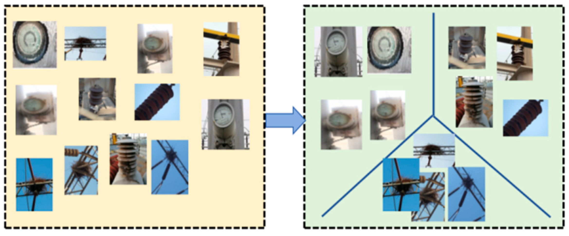
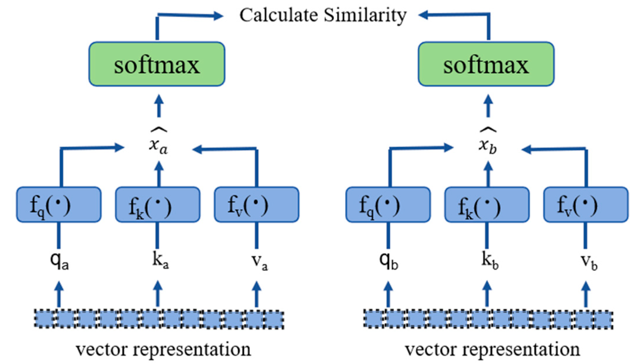
3.1. Global Self-Supervised Contrastive Loss

Global contrastive loss is utilized to enhance the similarity between different views of the same image while minimizing the similarity between views of different images. Assuming that two data augmentation methods are randomly applied to N samples { x i , y i } | i = 1 N in the meta-training set Dt, generating 2N augmented samples { x i ~ , y i ~ } | i = 1 N , { x ~ i , y ~ i } | i = 1 N , where x i ~ and x ~ i represent two different views of the original sample x i and are considered as positive pairs. Here, we define f as the feature extractor, which can transform the samples x i into feature maps x ^ i = f ( x i ~ ) R C × H × W   a n d   x ^ i = f ( x ~ i ) R C × H × W according to the learned parameters ϕ, and further obtain global features h i   a n d   h i R C through a pooling layer. A multi-layer perception is used to convert the global features into a vector, generating the projected vector z i = F C ( h i ) , z i = F C ( h i ) R D . Then, the global self-supervised contrastive loss can be calculated as:
L g l o b a l = i = 1 N l o g e x p ( z i · z i / τ ) j = 1 N e x p ( z i · z j / τ )
In the given context, the operation “·” represents the dot product after L2 normalization (The L2 norm is the square root of the sum of squares for absolute differences between feature vector coordinates.), where N is the number of images in a batch, τ is a temperature parameter used to control the penalty on negative samples, and the positive pair z i and z i consists of feature vectors extracted from the same sample x i through different augmentation methods.

3.2. Local Self-Supervised Contrastive Loss

Although the global loss function based on the global feature vector hi is beneficial for obtaining a global representation, it may overlook some local discriminative information in the feature maps, which can be more effective in small-sample learning. Therefore, this paper proposes a local self-supervised contrastive loss. Unlike previous methods, we utilize a local mapping module (referred to as Loc Map in Figure 2a) to enhance the robustness and generalization ability of the representation, with the specific module shown in Figure 3. Here, three spatial projection heads f q , f k , f v are used to project the local feature maps x ^ i into queries q i = f q ( x ^ i ) , keys k i = f k ( x ^ i ) , and values v i = f k ( x ^ i ) , respectively, where q i , k i , v i R H W × D . For a pair of local feature maps x ^ a and x ^ b , we align x ^ a and x ^ b to obtain v a | b = s o f t m a x ( q b k a T d ) v a , and align x ^ b with x ^ a to obtain v b | a = s o f t m a x ( q a k b T d ) v a . After L2 normalizing each position (i, j) in the aligned results, we can calculate the similarity between the two local feature maps, x ^ a and x ^ b , defined as follows:
s i m ( x ^ a , x ^ b ) = 1 H W i = 1 , j = 1 i = H , j = W ( v a | b ) i j T ( v b | a ) i j
The above formula calculates the similarity between two feature maps v a | b and v b | a (both belonging to R H W × D ). The self-supervised contrastive loss for the pair of feature maps can be computed as follows:
L l o c a l = i = 1 N l o g e x p ( s i m ( x ^ i · x ^ j ) / τ 1 ) j = 1 N e x p ( s i m ( x ^ i · x ^ j ) / τ 1 )
Here, ( x ^ i · x ^ j ) is a positive pair, i ≠ j, and τ 1 represents the temperature parameter. At the same time, we employ a local module to further mine the local contrastive information between instances, as shown in Figure 3. During the pre-training phase, we minimize the following loss:
L s t a g e 1 = α 1 L g l o b a l + α 2 L l o c a l
where α1 and α2 are weight factors that balance the global and local losses. By optimizing Lstage1, the model’s feature representation is enhanced in terms of discriminability and generalization, further preparing it for the next step of supervised fine-tuning.

3.3. Supervised Fine-Tune

In the first stage, through self-supervised learning, the model effectively utilizes a large number of unlabeled abnormal image samples. In the second stage, the model is provided with a limited number of samples, for example, only one sample or five samples per substation anomaly sample image. To better recognize substation anomaly samples, we employ a supervised contrastive learning approach and train it in conjunction with the image classification loss. We consider two images from the same category as positive pairs and two images from different categories as negative pairs for contrastive learning. The corresponding loss is as follows:
L c o n = 1 T i = 1 N j = 1 N 1 y i = y j l o g e x p ( c o s ( h i , h j ) / τ ) k = 1 N e x p ( c o s ( h i , h k ) / τ )
where T is the number of sample pairs from the same category within a batch. cos() refers to the cosine similarity between two vectors. The classification loss for the abnormal images is as follows:
L c l s = 1 N j = 1 C i = 1 N l o g P ( C j | x i )
where P ( C j | u i ) is the probability that the i-th image is predicted to have the j-th category. We jointly train these two losses in each batch:
L s t a g e 2 = β 1 L c o n + β 2 L c l s
where β 1 and β 2 are weight factors serving as hyperparameters.

4. Experimental Results and Discussion

4.1. Dataset of Abnormal Scenes in Substation

This study creates a dataset of abnormal scenarios encountered in substations, capturing instances of blurred dials, damaged dials, fractured insulators, ground oil contamination, closed cabinet doors, bird nests, damaged cover plates, abnormal meter readings, and discolored silicone, as illustrated in Figure 4. The other six classes include broken dial, discoloration of silica gel, broken insulator, abnormal closure of the cabinet door, suspended objects in the air, and not wearing a safety helmet. The dataset comprises a total of 3000 images, with each anomaly class containing 200 images. For the experimental setup, ten classes are chosen for the training set, and five classes are designated for the test set. No labels were used when constructing the pre-trained model.

4.2. Experimental Setup

In this experiment, Conv-4 [16] and ResNet-12 [8], widely used as backbone networks by researchers, are adopted for feature extraction. Conv-4 consists of four repeated convolutional blocks, each with a kernel size of 3, stride of 1, padding of 1 for convolutional layer, a BatchNorm layer, a ReLU function, and a size of 2 for max pooling layer. ResNet-12 has four residual blocks, each containing three convolutional layers, where “12” means a total of twelve convolutional layers. To prevent the impact of size differences on model performance, the image size in both the training and test sets is set to the same number of pixels. The network is trained using the Stochastic Gradient Descent (SGD) optimizer in the pre-training and meta-training fine-tuning stages. During pre-training (first stage) and meta-training (second stage), the weight decay and momentum are set to 4 × 10⁻⁴ and 0.8, respectively. During pre-training, the learning rate is initialized to 0.1 and adjusted using a cosine learning rate scheduler after a warm-up period. The training lasts for 20 epochs with a batch size of 64. The temperature parameters τ and τ1 are both set to 0.1. The weight factors α and β are set to 0.7 and 0.3, respectively, allowing the model to focus more on the global loss during the first pre-training stage. For different meta-learning fine-tuning tasks, the pre-trained model is fine-tuned with a 5-way 5-shot (5 training samples per class) and a 5-way 1-shot setting, with a batch size of 16 for a total of 30 epochs. The weight factors β 1 and β 2 are set to 0.2 and 0.8, respectively, with the loss function focusing more on the classification loss in the second stage. The entire model training is conducted on a single NVIDIA 3090 GPU with 24 GB of video memory. Data augmentation: for the constructed dataset, during the pre-training stage, various data augmentation strategies are used for contrastive learning, including image transformations such as random resized cropping, color jittering, and random horizontal flipping, as well as random grayscale conversion. In the second stage, during the fine-tuning of supervised contrastive learning, data augmentation is combined with data pairing strategies due to the limited amount of data.

4.3. Evaluation Metrics

In our experiment, the created dataset is a multi-class classification problem. The multi-class distribution of the test dataset cannot reflect the effect of the classificaton of few-shot learning. Therefore, binary classification experiments were carried out on the created dataset to make the evaluation fairer. The final classification results are divided into four states: TP (true positive), FP (false positive), TN (true negative), and FN (false negative). These are also four basic metrics of the confusion matrix. TP is the number of normal images classified in the normal scene. FP is the number of abnormal images incorrectly classified in the normal scene. TN is the number of abnormal images classified correctly. FN is the number of normal images classified in abnormal scenes. To evaluate the performance of the proposed method, four states—the accuracy, precision, detection rate, and false alarm rate—and F-measure are defined below:
A c c u r a c y = T P + T N T P + T N + F N + F P
P r e c i s i o n = T P T P + F P
R e c a l l = T P T P + F N
F 1 S c o r e = 2 ( P r e c i s i o n R e c a l l ) P r e c i s i o n + R e c a l l

4.4. Experimental Results

In this research, the binary classification, which has only two categories, namely normal and abnormal, is used to calculate the evaluation metrics. All evaluation metrics are reported as averaged results with 95% confidence intervals based on 30 experiments. This subsection presents the conducted meta-learning experiments, including 5-way 1-shot and 5-way 5-shot experiments, and reports the classification accuracy, precision, F1-score, and recall in percentage form. The feature extraction backbone networks are Conv-4 and ResNet-12. The detailed evaluation metric is calculated as shown in Table 1 and Table 2. Compared to other methods, 2-SCL significantly improves classification performance across various metrics. Since the data are balanced, in terms of accuracy, when Conv-4 and ResNet-12 are employed as the feature extraction backbone network, 2-SCL achieves a 12% and 10.57% improvement over RelationNet [16] in the 5-way 1-shot task and an 11.17% and 7.19% improvement in the 5-way 5-shot task. Under Conv-4, compared with the current top algorithm, 2-SCL improves accuracy by 1.64% in 5-way 1-shot and 1.21% in 5-way 5-shot. ResNet-12 improves accuracy by 0.52% in 5-way 1-shot and 1.53% in 5-way 5-shot. Other performance indicators also verify the same result. This indicates that 2-SCL can effectively enhance classification accuracy by utilizing the similarity of different attributes for classification. Although MatchingNets [12] and PrototypicalNets [18] are much better, their classification performance is not as good as that of 2-SCL. These results further demonstrate the proposed method’s effectiveness and superiority and the important role of two-stage training in meta-learning tasks. Additionally, as shown in Table 2, replacing the feature extraction network with a deeper network, ResNet-12, effectively improves classification accuracy. In the 5-way 5-shot task, 2-SCL can achieve an accuracy rate of 93.12%. This suggests that 2-SCL can effectively classify images to new categories under conditions of scarce samples, thus better adapting to the complex and variable environment of substations and being able to timely identify anomalies to prevent potential problems.

4.5. Ablation Experiments

We conducted ablation studies to investigate the effects of self-supervised contrastive pre-training and supervised contrastive fine-tuning. Table 3 shows the test results of the proposed model on the constructed dataset. The experimental results indicate that both stages are necessary, and the model can only achieve optimal performance by fine-tuning the pre-trained model. The self-supervised contrastive pre-training conducted in the first stage is indispensable, as all datasets have a significant drop in performance. The experiments demonstrate that contrastive pre-training algorithm with unlabel data, helps the model distinguish images with similar defects. Furthermore, performance also declines if supervised contrastive learning is not included in the small-sample fine-tuning phase. Specifically, in the 1-shot and 5-shot experiments, classification performance decreased by 4.56% and 3.32%, respectively; this is because the constructed dataset includes some similar defect images, where supervised contrastive learning can clearly differentiate images that are semantically similar but have limited training samples. The experiment also attempted to train the first and second stages together; however, compared to the proposed model structure, there was almost no improvement in recognition performance. Additionally, the experiment studied whether contrastive pre-training without including the test dataset aids in defect image recognition. Specifically, we performed pre-training using the training dataset in the first stage and used the test data for small-sample learning in the second stage. Compared to the model that did not undergo contrastive pre-training in the first stage, performance improved by 8.15% and 6.13% in the 1-shot and 5-shot settings, respectively. These improvements suggest that contrastive pre-training enhances recognition performance on the test dataset.
The proposed method can be abstracted into a multi-label classifier based on supervised contrastive meta-learning in the second stage, capable of simultaneously recognizing multiple attribute features within an image. Two loss functions are employed during training to enhance the model’s generalization and adaptability: the contrastive loss and the classification loss. The contrastive loss measures the model’s performance across all meta-learning tasks by calculating the discrepancy between the model’s predictions and the true labels, allowing the model to learn common features among different meta-learning tasks, thereby improving its generalization and adaptability. The classification loss, on the other hand, measures the model’s performance on each meta-learning task, enabling the model to learn the commonalities and differences between different samples and to understand the relationships between the intrinsic attribute features of each sample. Subsequently, ablation studies were conducted to explore the roles of these two losses. The model’s accuracy on the test set was observed when the contrastive and classification losses were removed separately. As shown in Table 4, the removal of either loss led to a decrease in accuracy to varying degrees. Taking the Conv-4 backbone as an example, the accuracy dropped by approximately 10% when only the contrastive loss was included. However, relying solely on contrastive loss is insufficient because it overlooks the mutually exclusive attribute features between different samples, leading to decreased accuracy. Meanwhile, including only the classification loss causes the network to focus solely on the attribute feature relationships between categories within each meta-learning task, failing to learn broader feature relationships based on global features. Although this allows the model to learn the relationships between each sample’s intrinsic attribute features, improving its accuracy and sensitivity, the global features are neglected, resulting in the failure to further enhance the recognition performance.The contrastive features are shared across all meta-learning tasks, enabling the model to learn a wider range of feature relationships and thus enhancing its generalization ability. Additionally, the same pattern applies to the ResNet-12 backbone, which once again confirms the effectiveness of using both contrastive loss and classification loss during training.

4.6. Parameter Sensitivity Experiment

In this subsection, we also investigated the impact of hyperparameters in contrastive learning, specifically the temperature parameters τ and τ1, as well as the weight factors α and β. We set τ and τ1 to be within the range {0.05, 0.1, 0.3, 0.5} {0.05, 0.1, 0.3, 0.5} and α 1 + α 2 = 1. Experimental results showed that τ and τ1 significantly affect the performance during the first stage of self-supervised contrastive pre-training. Additionally, we found that a batch size greater than 32 performs well in the pre-training phase. However, in the few-shot fine-tuning phase, setting τ to a smaller value of 0.05, which strongly increases the penalty on hard negative samples, β 1 + β 2 = 1, β 1 to a smaller value, and β 2 to a larger one significantly improves the model’s classification performance. This is because it increases the weight of the supervised contrastive learning loss. Moreover, the batch size also affects performance in this stage. Therefore, when the number of training samples is limited, the supervised contrastive loss is sensitive to hyperparameters. In the fine-tuning stage of model training, β 1 was set to 0.2, 0.4, 0.6, and 0.8 to explore its role as a hyperparameter. Table 5 summarizes the results of the few-shot learning classification. The choice of β 1 has a certain impact on the classification results. Taking the Conv-4 backbone as an example, the highest classification accuracy was achieved when β 1 was set to 0.4, with the 5-way 1-shot experimental result being 73.76%. As β 1 increases, the experimental results gradually deteriorate, which may be due to overfitting. The backbone ResNet-12 also shows the same trend, achieving the best performance when β 1 is 0.4, followed by a decline in classification accuracy as   β 1 increases. In this study, β 1 is set to 0.4 by default, and β 2 is set to 0.6.

5. Conclusions

This research presents a two-stage contrastive learning model (2-SCL) for abnormal substation scene identification. We constructed a dataset covering diverse abnormal conditions to address the scarcity of abnormal scene data in substations. 5-way 1-shot and 5-way 5-shot meta-learning experiments were conducted on this dataset, and the model performance was evaluated using metrics based on the confusion matrix. Experimental results show that the proposed 2-SCL method is superior. When using Conv-4 and ResNet-12 as the backbone network, 2-SCL improves accuracy over RelationNet by 12% and 10.57% in 5-way 1-shot and 11.17% and 7.19% in 5-way 5-shot. Even when compared with State-of-the-Art algorithms, 2-SCL exhibits better classification performance across all evaluation metrics. Ablation experiments confirm the importance of both pre-training and fine-tuning stages. The experimental results show that contrastive pre-training improves recognition performance on the test dataset, and using both contrastive loss and classification loss in training enables the model to learn a broader range of feature relationships, thus enhancing its generalization ability. This research advances State-of-the-Art substation abnormal detection and provides a feasible solution for the automated detection of substation abnormal scenes. Enhancing the accuracy and reliability of abnormal scene recognition contributes to the overall safety and stability of substation operations.

Author Contributions

Conceptualization, J.Z. and H.B.; methodology, H.S.; software, W.M.; data curation, M.L.; writing—original draft preparation, H.S. and S.L.; writing—review and editing, J.Z.; supervision, H.B.; project administration, H.B. All authors have read and agreed to the published version of the manuscript.

Funding

This research received no external funding.

Data Availability Statement

The original contributions presented in the study are included in the article, further inquiries can be directed to the corresponding author.

Conflicts of Interest

Author Haitao Su was employed by the State Grid Henan Electric Power Company. The remaining authors declare that the research was conducted in the absence of any commercial or financial relationships that could be construed as a potential conflict of interest.

References

  1. Ge, L.; Li, Y.; Li, Y.; Yan, J.; Sun, Y. Smart distribution network situation awareness for high-quality operation and maintenance: A brief review. Energies 2022, 15, 828. [Google Scholar] [CrossRef]
  2. Yan, X.; Liu, Y.; Xu, Y.; Jia, M. Multichannel fault diagnosis of wind turbine driving system using multivariate singular spectrum decomposition and improved Kolmogorov complexity. Renew. Energy 2021, 170, 724–748. [Google Scholar] [CrossRef]
  3. Kong, Y.; Jing, M. An Identification Method of Abnormal Patterns for Video Surveillance in Unmanned Substation; IEEE: Piscataway, NJ, USA, 2011. [Google Scholar]
  4. Wu, Y.; Xiao, F.; Liu, F.; Sun, Y.; Deng, X.; Lin, L.; Zhu, C. A Visual Fault Detection Algorithm of Substation Equipment Based on Improved YOLOv5. Appl. Sci. 2023, 13, 11785. [Google Scholar] [CrossRef]
  5. Gao, T.; Zhang, X. Investigation into recognition technology of helmet wearing based on HBSYOLOX-s. Appl. Sci. 2022, 12, 12997. [Google Scholar] [CrossRef]
  6. Xu, C.; Ni, D.; Wang, B.; Wu, M.; Gan, H. Two-stage anomaly detection for positive samples and small samples based on generative adversarial networks. Multimed. Tools Appl. 2023, 82, 20197–20214. [Google Scholar] [CrossRef]
  7. Sun, Q.; Liu, Y.; Chua, T.S.; Schiele, B. Meta-transfer learning for few-shot learning. In Proceedings of the IEEE/CVF Conference on Computer Vision and Pattern Recognition, Long Beach, CA, USA, 15–20 June 2019. [Google Scholar]
  8. Oreshkin, B.; Rodríguez López, P.; Lacoste, A. Tadam: Task dependent adaptive metric for improved few-shot learning. Adv. Neural Inf. Process. Syst. 2018, 31, 1–11. [Google Scholar]
  9. Sohn, K. Improved deep metric learning with multi-class N-pair loss objective. Adv. Neural Inf. Process. Syst. 2016, 29, 1–9. [Google Scholar]
  10. Su, J.C.; Maji, S.; Hariharan, B. When Does Self-supervision Improve Few-shot Learning. In European Conference on Computer Vision; Springer International Publishing: Cham, Switzerland, 2019. [Google Scholar]
  11. Koch, G.; Zemel, R.; Salakhutdinov, R. Siamese neural networks for one-shot image recognition. In Proceedings of the 32nd International Conference on Machine, Learning, Lille, France, 6–11 July 2015. [Google Scholar]
  12. Vinyals, O.; Blundell, C.; Lillicrap, T.; Wierstra, D. Matching Networks for One Shot Learning. Adv. Neural Inf. Process. Syst. 2016, 29, 1–9. [Google Scholar]
  13. Hou, R.; Chang, H.; Ma, B.; Shan, S.; Chen, X. Cross attention network for few-shot classification. Adv. Neural Inf. Process. Syst. 2019, 32, 1–12. [Google Scholar]
  14. Ye, H.J.; Hu, H.; Zhan, D.C.; Sha, F. Few-shot learning via embedding adaptation with set-to-set functions. In Proceedings of the IEEE/CVF Conference on Computer Vision and Pattern Recognition, Seattle, WA, USA, 14–19 June 2020. [Google Scholar]
  15. Lim, J.Y.; Lim, K.M.; Ooi, S.Y.; Lee, C.P. Efficient-prototypicalnet with self knowledge distillation for few-shot learning. Neurocomputing 2021, 459, 327–337. [Google Scholar] [CrossRef]
  16. Sung, F.; Yang, Y.; Zhang, L.; Xiang, T.; Torr, P.H.; Hospedales, T.M. Learning to compare: Relation network for few-shot learning. In Proceedings of the IEEE Conference on Computer Vision and Pattern Recognition, Salt Lake City, UT, USA, 18–23 June 2018. [Google Scholar]
  17. Zhang, X.; Qiang, Y.; Sung, F.; Yang, Y.; Hospedales, T.M. RelationNet2: Deep comparison columns for few-shot learning. arXiv 2018, arXiv:1811.07100. [Google Scholar]
  18. Snell, J.; Swersky, K.; Zemel, R. Prototypical networks for few-shot learning. Adv. Neural Inf. Process. Syst. 2017, 30, 1–11. [Google Scholar]
  19. Bertinetto, L.; Henriques, J.F.; Torr, P.H.; Vedaldi, A. Meta-learning with differentiable closed-form solvers. arXiv 2018, arXiv:1805.08136. [Google Scholar]
  20. Alexey, D.; Fischer, P.; Tobias, J.; Springenberg, M.R.; Brox, T. Discriminative unsupervised feature learning with exemplar convolutional neural networks. IEEE TPAMI 2016, 38, 1734–1747. [Google Scholar]
  21. Gidaris, S.; Singh, P.; Komodakis, N. Unsupervised representation learning by predicting image rotations. arXiv 2018, arXiv:1803.07728. [Google Scholar]
  22. Doersch, C.; Gupta, A.; Efros, A.A. Unsupervised visual representation learning by context prediction. In Proceedings of the IEEE International Conference on Computer Vision, Nashville, TN, USA, 11–15 June 2015. [Google Scholar]
  23. Pathak, D.; Krahenbuhl, P.; Donahue, J.; Darrell, T.; Efros, A.A. Context encoders: Feature learning by inpainting. In Proceedings of the IEEE Conference on Computer Vision and Pattern Recognition, Las Vegas, NV, USA, 27–30 June 2016. [Google Scholar]
  24. Zhang, R.; Isola, P.; Efros, A.A. Split-brain autoencoders: Unsupervised learning by cross-channel prediction. In Proceedings of the IEEE Conference on Computer Vision and Pattern Recognition, Honolulu, HI, USA, 21–26 July 2017. [Google Scholar]
  25. Chopra, S.; Hadsell, R.; LeCun, Y. Learning a similarity metric discriminatively, with application to face verification. In Proceedings of the IEEE Computer Society Conference on Computer Vision and Pattern Recognition (CVPR’05), San Diego, CA, USA, 20–25 June 2005. [Google Scholar]
  26. Schroff, F.; Kalenichenko, D.; Philbin, J. Facenet: A unified embedding for face recognition and clustering. In Proceedings of the IEEE Conference on Computer Vision and Pattern Recognition, Boston, MA, USA, 7–12 June 2015. [Google Scholar]
  27. Lee, H.; Hwang, S.J.; Shin, J. Self-supervised label augmentation via input transformations. In Proceedings of the International Conference on Machine Learning, Online, 13–18 July 2020. [Google Scholar]
  28. Chen, D.; Chen, Y.; Li, Y.; Mao, F.; He, Y.; Xue, H. Self-supervised learning for few-shot image classification. In Proceedings of the ICASSP 2021-2021 IEEE International Conference on Acoustics, Speech and Signal Processing (ICASSP), Toronto, ON, Canada, 6–11 June 2021. [Google Scholar]
  29. Yang, Z.; Wang, J.; Zhu, Y. Few-shot classification with contrastive learning. In European Conference on Computer Vision; Springer: Berlin/Heidelberg, Germany, 2022. [Google Scholar]
Figure 1. Distribution of Samples in the Feature Space After Contrastive Learning.
Energies 17 06282 g001
Figure 2. The Network Framework, (a) The Pre-training Framework of the First Stage, (b) The Fine-tuning Framework of the Second Stage.
Energies 17 06282 g002
Figure 3. Local Map Module.
Energies 17 06282 g003
Figure 4. Example of substation anomalies. (The last image is an example of abnormal meter readings).
Energies 17 06282 g004
Table 1. Results of substation anomaly detection with Conv-4 as the backbone.
BackboneMethods5-Way 1-Shot5-Way 5-Shot
AccuracyPrecisionF1-ScoreRecallAccuracyPrecisionF1-ScoreRecall
Conv-4RelationNets [16]61.76 ± 0.4858.32 ± 0.8157.5 ± 0.4356.71 ± 0.5477.59 ± 0.7368.27 ± 0.7870.52 ± 0.8172.93 ± 0.76
MatchingNets [12]64.52 ± 0.6756.14 ± 0.6359.13 ± 0.5262.45 ± 0.780.63 ± 0.5373.37 ± 0.5472.55 ± 0.6571.76 ± 0.64
PrototypicalNets [18]67.67 ± 0.5856.21 ± 0.5960.84 ± 0.5966.31 ± 0.6382.39 ± 0.4274.15 ± 0.6173.32 ± 0.7372.5 ± 0.75
R2D2 [19]69.56 ± 0.4262.6 ± 0.5364.94 ± 0.7267.47 ± 05187.65 ± 0.6364.86 ± 0.6573.9 ± 0.7285.89 ± 0.76
RelationNets2 [17]72.12 ± 0.8264.9 ± 1.2167.66 ± 0.9370.67 ± 0.3685.49 ± 0.5979.5 ± 0.6376.39 ± 0.5873.52 ± 0.65
2-SCL (ours)73.76 ± 0.5667.85 ± 0.4869.64 ± 0.5171.54 ± 0.4688.76 ± 0.5682.54 ± 0.5584.29 ± 0.5486.13 ± 0.51
Table 2. Results of substation anomaly detection with ResNet-12 as the backbone.
BackboneMethods5-Way 1-Shot5-Way 5-Shot
AccuracyPrecisionF1-ScoreRecallAccuracyPrecisionF1-ScoreRecall
ResNet-12RelationNets [16]72.56 ± 0.6361.67 ± 0.7565.23 ± 0.6769.23 ± 0.5985.93 ± 0.4974.75 ± 0.7770.67 ± 0.7267.02 ± 0.74
MatchingNets [12]75.91 ± 0.4972.18 ± 0.4771.87 ± 0.4671.58 ± 0.5388.37 ± 0.6982.18 ± 0.6180.37 ± 0.6378.64 ± 0.64
PrototypicalNets [18]76.43 ± 0.5277.12 ± 0.4375.08 ± 0.4873.15 ± 0.5189.61 ± 0.8385.12 ± 0.7282.82 ± 0.7680.64 ± 0.81
TADAM [8]81.72 ± 0.6774.32 ± 0.6877.19 ± 0.5980.3 ± 0.5790.72 ± 0.7277.11 ± 0.6780.62 ± 0.6384.46 ± 0.66
R2D2 [19]82.61 ± 0.7381.23 ± 0.7879.5 ± 0.7277.85 ± 0.7191.59 ± 0.5185.18 ± 0.5882.83 ± 0.5680.6 ± 0.54
2-SCL (ours)83.13 ± 0.4984.35 ± 0.4882.77 ± 0.4681.25 ± 0.4293.12 ± 0.6486.6 ± 0.5287.97 ± 0.589.39 ± 0.48
Table 3. Testing accuracy (×100%) under different settings.
Model5-Way 1-Shot5-Way 5-Shot
(ours)83.83 ± 0.5793.12 ± 0.43
w/o Contrastive pre-training−8.15−6.13
w/o Supervised contrastive learning−4.56−3.32
w/o Contrastive pre-training + w/o Supervised contrastive learning−9.35−7.69
Table 4. Results of ablation experiments of different loss components.
BackboneContrastive LossClassification Loss5-Way 1-Shot5-Way 5-Shot
Conv-4×62.43 ± 0.9675.32 ± 0.87
×71.29 ± 0.4285.91 ± 0.62
73.76 ± 0.5688.76 ± 0.56
ResNet-12×73.89 ± 0.4582.19 ± 0.61
×79.47 ± 0.6888.40 ± 0.55
83.83 ± 0.5793.12 ± 0.43
“×” and “√” indicate that the model does not contain and contain the corresponding loss respectively.
Table 5. Results of different coefficient β 1 for 2-SCL.
Backbone β 1 5-Way 1-Shot5-Way 5-Shot
Conv-40.272.53 ± 0.8286.37 ± 0.63
0.473.76 ± 0.5688.76 ± 0.56
0.6 71.61 ± 0.4284.30 ± 0.67
0.872.66 ± 0.1585.81 ± 0.72
ResNet-120.280.18 ± 0.4989.29 ± 0.54
0.483.83 ± 0.5793.12 ± 0.43
0.683.44 ± 0.5892.89 ± 0.50
0.883.01 ± 0.6091.94 ± 0.49
Disclaimer/Publisher’s Note: The statements, opinions and data contained in all publications are solely those of the individual author(s) and contributor(s) and not of MDPI and/or the editor(s). MDPI and/or the editor(s) disclaim responsibility for any injury to people or property resulting from any ideas, methods, instructions or products referred to in the content.

