Cooperative Control Strategy for Power Quality Based on Heterogeneous Inverter Parallel System

Abstract

Multi-functional grid-connected inverters (MFGCIs) have attracted much attention for their auxiliary services to improve power quality in microgrids and new energy generation systems. However, power quality enhancement based on MFGCIs often only considers a single control method. The regulation potential of multiple control-type inverters is not fully utilized. To suppress harmonic and support voltage, a cooperative control strategy based on the parallel system of a grid-following (GFL) inverter and a grid-forming (GFM) inverter is proposed. The topology of the MFGCIs is introduced and a mathematics model is deduced. Secondly, a specific-order harmonic compensation method is proposed for the harmonic suppression at the point of common coupling (PCC). The harmonic current is realized to be shared according to the inverter capacity. The reactive power output of the heterogeneous inverters is coordinated by calculating the reactive power compensation and reactive power allocation so that the PCC voltage always stays near the rated voltage. Finally, the effectiveness of the proposed control strategy is verified by simulation and experiment.

1. Introduction

Distributed generation based on renewable energy sources has been greatly developed due to its advantages of low cost, local use of electricity, and low transmission losses [1,2,3]. At the same time, a large number of power electronic devices and non-linear loads are connected to the grid, which will lead to increasingly serious power quality problems at the point of common coupling (PCC) [4,5].

Traditional power quality enhancement devices, such as active power filters, unified power quality regulators, and static reactive power generators, have been widely used due to their advantages of flexibility, controllability, and versatility [6,7]. However, the use of additional power quality compensators increases the investment costs and maintenance costs [8]. Grid-connected inverters (GCIs) have a similar topology to power quality control devices [9]. Therefore, multi-functional grid-connected inverters (MFGCIs) [10,11,12], which combine filtering and reactive power compensation, are widely explored. In [10], a comprehensive review on the topologies and control strategies of MFGCIs is provided. MFGCIs have the ability to provide auxiliary reactive power and harmonics compensation in grid-connected mode and an uninterrupted power supply mode to loads during grid outages [11]. By introducing a space-vector pulse-width modulation strategy, the MFGCIs enable active power transfer with higher efficiency, while maintaining the ability to implement maximum power tracking and improve power quality [12]. MFGCIs increase the utilization of inverter capacity and reduce equipment coverage and investment and maintenance costs.

The existing research on MFGCIs for harmonic suppression mainly focuses on detection methods, tracking, and control strategies for harmonics. The instantaneous power-based method can effectively detect low harmonics, but the method is affected by the performance of the phase-locked loop (PLL) and the low-pass filter [13]. To solve the problem arising from PLL, a detection method based on conservative power theory has been further proposed, but its calculation is complicated [14,15]. To reduce the effect of the low-pass filter, the adaptive harmonic detection method is proposed [16], which can improve the detection accuracy of harmonic currents. However, it is more complicated to calculate.

For the tracking control of harmonics, the commonly used controllers include the proportional integral controller (PI), the proportional resonance controller (PR) [17], and so on. Since the reference current of an MFGCI also contains harmonic and reactive commands, it is difficult for the PI controller to achieve low steady-state error tracking [18]. Therefore, the traditional PI control in the rotating coordinate system is no longer applicable. PR controllers enable the highly accurate tracking of the frequency-specific AC component but are complex to apply. Compared with the above controllers, control methods such as quasi-resonant control (QRC) and repetitive control (RC) have been widely used due to their robustness. QPR based on the internal model of single-frequency AC signal can achieve high open-loop gain at the fundamental frequency of the system. By using multiple quasi-resonant links in parallel, it can achieve high gain at multiple harmonic frequencies. It is a commonly used harmonic suppression method [19,20]. RC based on the internal model principle can achieve high system open-loop gain at fundamental and harmonic frequencies, which is very suitable for the output voltage harmonic suppression of inverters [21,22]. However, RC has a periodic delay link, and the dynamic characteristics of the system are poor.

GCIs can be classified into grid-following (GFL) inverters and grid-forming (GFM) [23] inverters according to their control method. GFL control is flexible and has a fast power response [24]. GFM inverters have attracted widespread attention in recent years on account of their frequency and voltage support capability [25]. Generally, MFGCIs only consider a single control method and have not fully utilized the benefits of the two types of inverters. As the proportion of GFM inverters increases, research on the cooperative strategy of GFL and GFM is necessary to improve the power quality of the grid [26].

At present, the existing research on GFL and GFM synergy still focuses on small disturbance stability analysis, transient stability, and the optimal configuration of the GFL and GFM inverter ratio. In [27], the stability of the interacting system of GFM and GFL inverters is analyzed; however, it only evaluates the robust stability under different types of converter combination conditions. In [28,29], the transient stability of a two-machine system, consisting of a GFM and a synchronous generator, and a GFM and a GFL, respectively, was investigated. In terms of optimal configuration, the capacity constraints, voltage constraints, and static stability constraints of the grid-connected system of the GFL/GFM converter are comprehensively considered, and the optimal configuration method of the GFL/GFM converter to satisfy the oscillatory stability constraints of the full operation domain is proposed in [30]. To regulate the voltage of both inverters to the same range, a cooperative control study of grid-forming and grid-following inverters was presented by the authors of [26]. However, there is a lack of research on the synergy of GFL and GFM for power quality control. Therefore, combining the advantages of GFL and GFM is important to improve power quality.

Firstly, the fundamental structure and control strategy of the parallel system are introduced. Secondly, to suppress the current harmonics and support voltage at the PCC, a cooperative strategy for the GFL and GFM inverters is proposed. Finally, the effectiveness of the proposed strategy is verified by simulation analysis.

2. Constitution of the Parallel System

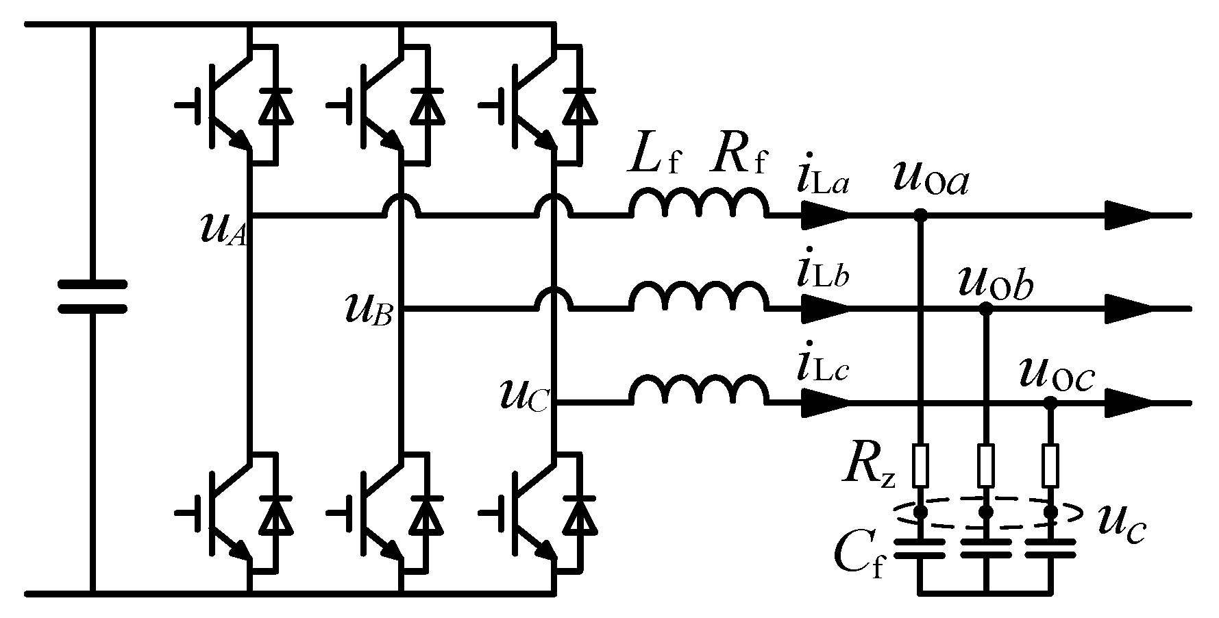
2.1. Topology and Modeling of the Inverters

In this paper, both GFL and GFM inverters use three-phase two-level inverter topology, and are connected to the grid through an LC filter, as shown in Figure 1.

The mathematical model of GCI in rotating frame is expressed as:

$$\left\{\begin{array}{c}{u}_{\mathrm{o}d}=\left(1+R_{\mathrm{z}}{C}_{\mathrm{f}}s\right)u_{\mathrm{c}d}-R_{\mathrm{z}}\omega C_{\mathrm{f}}{u}_{\mathrm{c}q}\\ u_{\mathrm{o}q}=\left(1+R_{\mathrm{z}}{C}_{\mathrm{f}}s\right)u_{\mathrm{c}q}+R_z\omega C_{\mathrm{f}}{u}_{\mathrm{c}d}\end{array}\right.$$

(1)

where u_cq and u_cd can be expressed as:

$$\left\{\begin{array}{l}{u}_{\mathrm{c}q}={\displaystyle \frac{s{i}_{\mathrm{L}q}-s{i}_{\mathrm{o}q}-\left(\omega i_{\mathrm{L}d}-\omega i_{\mathrm{o}d}\right)}{C_{\mathrm{f}}\left(s^2+{\omega }^2\right)}}\\ u_{\mathrm{c}d}={\displaystyle \frac{\omega i_{\mathrm{L}q}-\omega i_{\mathrm{o}q}+s{i}_{\mathrm{L}d}-s{i}_{\mathrm{o}d}}{C_{\mathrm{f}}\left(s^2+{\omega }^2\right)}}\end{array}\right.$$

(2)

where i_Ld and i_Lq are the d q-axis components of the inverter side current, respectively; i_od and i_oq are the output current d q-axis components; u_od and u_oq represent the output voltage d q-axis components; u_cd and u_cq are the capacitance voltage d q-axis components; and ω is the grid angular frequency.

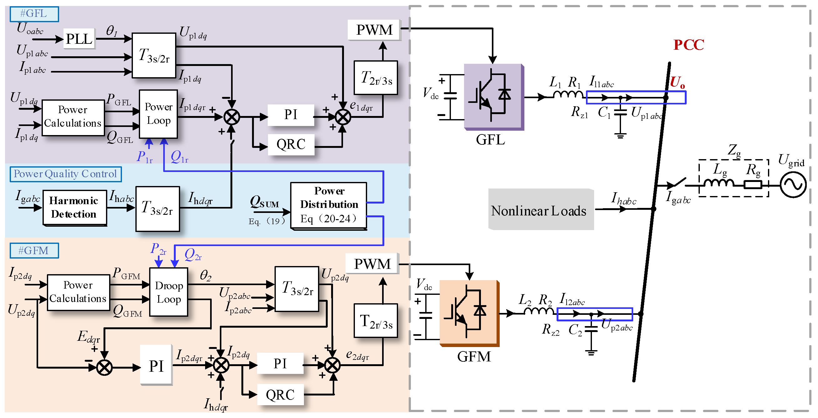
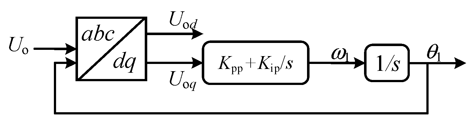
2.2. Structure and Basic Control Strategy of Parallel System

Figure 2 shows the structure and control strategy of the parallel system.

In Figure 2, Z_g is the grid impedance; I_l1/I_l2 are the GFL and GFM inverter filter inductor current, respectively; U_p1/U_p2 are the GFL and GFM filter capacitor voltage, respectively; U_o is the voltage of PCC; U_grid and I_grid are the grid voltage and grid current, respectively; T_3s/2r is the transformation of a three-phase stationary frame to a two-phase rotating frame; and T_2r/3s is the corresponding inverse transformation matrix. In this paper, the DC voltage is considered as a constant value.

The GFL inverter uses PLL for coordinate transformation and synchronization. Figure 3 shows the basic structure of PLL. The output angle θ₁ of PLL can be expressed as:

$${\theta }_1={\displaystyle \frac{\omega }{s}}={\displaystyle \frac{1}{s}}\left[G_{\mathrm{PLL}}\left(s\right)U_{\mathrm{o}q}+{\omega }_0\right]$$

(3)

where G_PLL(s) = K_pp + K_ip/s is the PI controller of the PLL and ω₀ is the rated angular frequency.

In Figure 3, ω₁ is the angular frequency of the GFL inverter; K_pp is the proportionality coefficient for PLL; and K_ip is the integral coefficient for PLL.

The GFL inverter uses PQ power control, which can be expressed as

$$\left\{\begin{array}{l}{I}_{1d\mathrm{r}}=G_{\mathrm{p}}(s)(P_{1\mathrm{r}}-P_{\mathrm{GFL}})\\ I_{1q\mathrm{r}}=G_{\mathrm{p}}(s)(Q_{\mathrm{GFL}}-Q_{1\mathrm{r}})\end{array}\right.$$

(4)

where G_p(s) is the PI controller of the power outer loop; P_1r is the active power reference of GFL; Q_1r is the reactive power reference of GFL; P_GFL is the active power output of GFL; and Q_GFL is the reactive power output of GFL. To suppress harmonics, the d and q axis components of the harmonic command I_hdqr are superimposed with the d and q axis components of the fundamental command I_p1dqr and they are involved in the current feedback control. In the current inner loop, the PI controller parallels the QRC controller to accurately track the superimposed current commands.

According to Figure 3, the GFM inverter applies the droop control strategy. I_l2 and U_p2 are fed to the outer loop of the GFM inverter by the power calculation module. The droop loop of the GFM inverter generates the reference voltage and phase of the inner loop. The inner loop of the GFM inverter outputs the dq-axis reference voltage of the inverter, which is fed to the GCI after the coordinate transformation and PWM. The typical control structure and expression of a droop control are shown in Figure 4 and Equation (5), respectively.

In Figure 4, ω₂ is the angular frequency of the GFM inverter.

$$\left\{\begin{array}{l}{\omega }_2=k_{\mathrm{p}}\left(P_{2\mathrm{r}}-P_{\mathrm{GFM}}\right)+{\omega }_{\mathrm{N}}\\ E_{\mathrm{r}}=k_{\mathrm{q}}\left(Q_{2\mathrm{r}}-Q_{\mathrm{GFM}}\right)+V_{\mathrm{N}}\end{array}\right.$$

(5)

where P_GFM/Q_GFM and P_2r/Q_2r are the output active/reactive power actual and reference values, respectively; V_N and ω_N are the rated voltage and rated angular frequency; and k_p and k_q are the droop coefficients of active power and reactive power loop, respectively.

3. Harmonic Suppression Strategy

In addition to the transmission power, the heterogeneous parallel system has the auxiliary capability for harmonic suppression. When non-linear loads are connected to the grid, the harmonic suppression strategy is required for the power quality of the output current of heterogeneous inverter parallel system. In this paper, both the GFL and GFM inverters have the function of harmonic compensation.

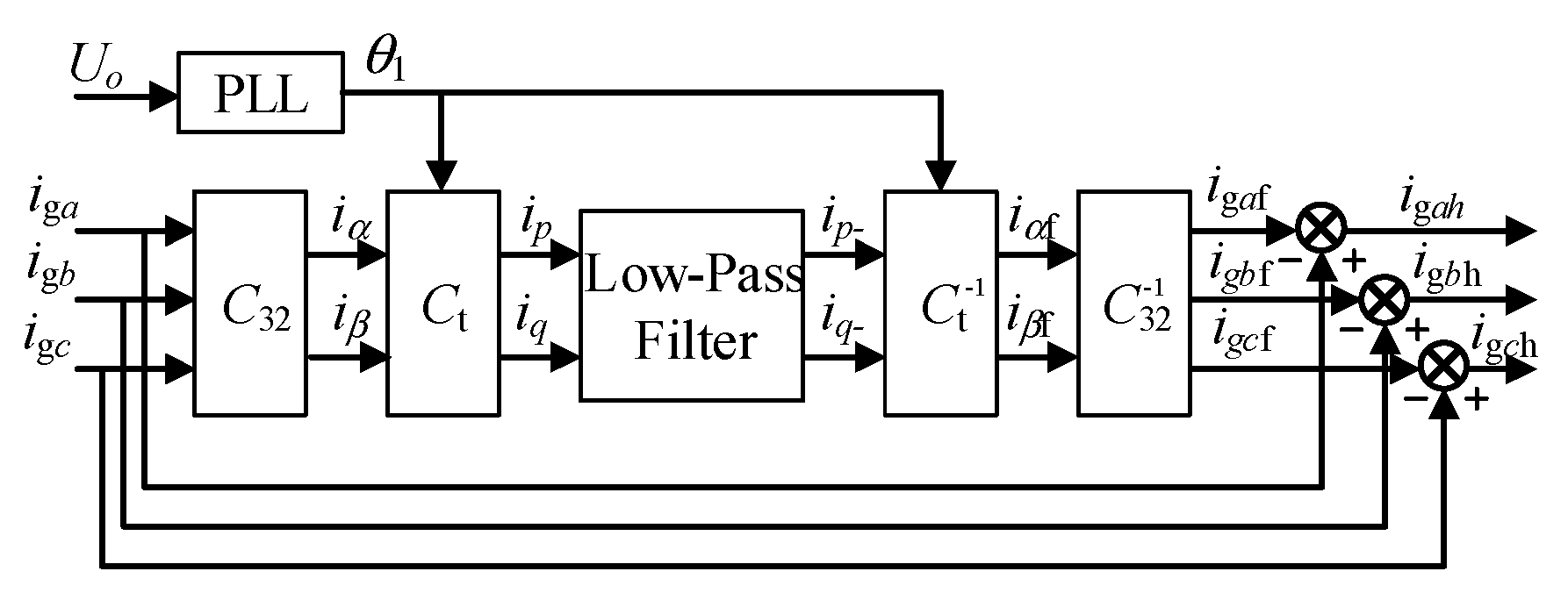
3.1. Detection of Harmonic Current

The accurate detection of harmonic current is a prerequisite for harmonic suppression. The principle of the harmonic detection method is shown in Figure 5.

In Figure 5, i_p and i_q are the instantaneous active current and instantaneous reactive current, respectively; i_p- and i_q- are the DC components of i_p and i_q, respectively; i_α and i_β are the instantaneous currents in the two-phase stationary frame; i_αf and i_βf are the fundamental components of the load current i_α and i_β, respectively; i_gaf, i_gbf, and i_gcf are the fundamental currents of the three-phase grid current, respectively; and i_gah, i_gbh, and i_gch are the harmonic currents of the three-phase grid current, respectively.

Firstly, the three-phase grid current is transformed to the αβ frame system to obtain i_α and i_β by the frame transformation matrix C₃₂. Then, i_α and i_β are transformed to i_p and i_q in the dq coordinate system by the matrix C_t. The matrix C_t and the current i_p, i_q are shown in (7) and (8).

$$C_{32}=\sqrt{{\displaystyle \frac{2}{3}}}\left[\begin{array}{ccc}1& -{\displaystyle \frac{1}{2}}& -{\displaystyle \frac{1}{2}}\\ 0& {\displaystyle \frac{\sqrt{3}}{2}}& -{\displaystyle \frac{\sqrt{3}}{2}}\end{array}\right]$$

(6)

$$C_{\mathrm{t}}=\left[\begin{array}{cc}\cos \omega t& \sin \omega t\\ -\sin \omega t& \cos \omega t\end{array}\right]$$

(7)

$$\left[\begin{array}{c}{i}_p\\ i_q\end{array}\right]=\sqrt{3}\left[\begin{array}{c}{\displaystyle \sum _{\tau =1}^{\infty }\pm i_{\tau }\cos \left[\left(\mp 3n\right)\omega t\mp {\phi }_{\tau }\right]}\\ {\displaystyle \sum _{\tau =1}^{\infty }\pm i_{\tau }\sin \left[\left(\mp 3n\right)\omega t\mp {\phi }_{\tau }\right]}\end{array}\right]$$

(8)

where τ is the order of harmonic and τ = 3n ± 1. In the equation, the upper sign is taken when τ = 3n + 1, and the lower sign is taken when τ = 3n − 1. Typical harmonic sources in the grid are three-phase uncontrolled rectified loads, which mainly contain 6n ± 1 (n = 1, 2, 3, …) harmonics. To filter out the 6n ± 1th harmonic current in the three-phase load current, the current command can be expressed as

$$\left[\begin{array}{c}{i}_p\\ i_q\end{array}\right]=\sqrt{3}\left[\begin{array}{c}{\displaystyle \sum _{\tau =1}^{\infty }\pm i_{\tau }\cos \left[\left(\mp 6n\right)\omega t\mp {\phi }_{\tau }\right]}\\ {\displaystyle \sum _{\tau =1}^{\infty }\pm i_{\tau }\sin \left[\left(\mp 6n\right)\omega t\mp {\phi }_{\tau }\right]}\end{array}\right]$$

(9)

where τ is the order of harmonics and τ = 6n ± 1. In the equation, the upper sign is taken when τ = 6k + 1, and the lower sign is taken when τ = 6k − 1.

After calculating i_p and i_q, i_p− and i_q− can be obtained using the low-pass filter. i_p− and i_q− can be expressed as:

$$\left[\begin{array}{c}{i}_{p-}\\ i_{q-}\end{array}\right]=\left[\begin{array}{c}\sqrt{3}{I}_1\cos (-{\phi }_1)\\ \sqrt{3}{I}_1\sin (-{\phi }_1)\end{array}\right]$$

(10)

Then, the fundamental components of the grid current are obtained by the inverse transformation of C_t and C₃₂. Finally, the harmonic of all loads can be obtained from the difference between i_gaf, i_gbf, and i_gcf and i_ga, i_gb, and i_gc.

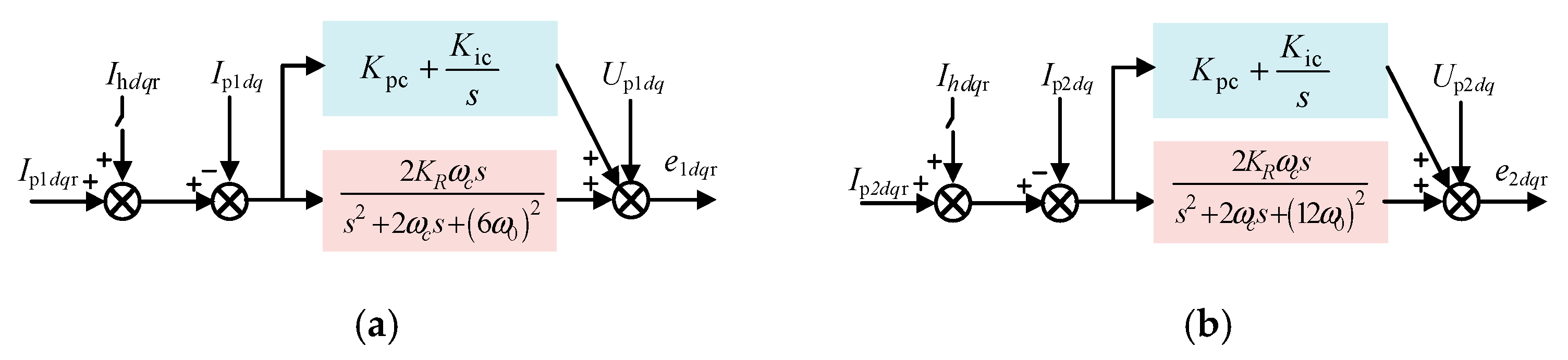
3.2. Tracking and Harmonic Current Allocation of Composite Commands

The PI controller tracks the DC component without static error, while it is difficult to accurately track the superimposed command. The QRC controller has infinite gain at the resonance frequency, which keeps the steady-state error of the AC component at zero. Therefore, the PI controller in parallel with the QRC controller can be used for improving the tracking performance of the compound command.

The transfer function of the QRC controller is shown in (11)

$$G\left(s\right)={\displaystyle \frac{2K_R{\omega }_{\mathrm{c}}s}{s^2+2{\omega }_{\mathrm{c}}s+{\omega }_x^2}}$$

(11)

where K_R is the integration coefficient, ω_x is the resonant frequency of the resonant controller, and ω_c is the controller cut-off frequency.

The coordinate transformation makes the nth harmonic in the three-phase stationary coordinate system into the (n − 1)th component and the (n + 1)th component in the dq-coordinate. Therefore, the 5th and 7th harmonics need to be tracked in the dq coordinate system using a QRC with a resonant frequency of 6 times the fundamental frequency.

Considering the limitation of the capacity, this paper mainly focuses on the compensation of low harmonics such as 5th, 7th, 11th, and 13th harmonics. Due to the differences in capacity and operating conditions, this paper proposes a specific-order harmonic compensation method to achieve harmonic capacity allocation. The harmonic magnitude is usually inversely related to the order of harmonics. In this paper, the GFL inverter has a larger capacity and the GFM inverter has a smaller capacity. Therefore, in the GFL inverter, a QRC resonant controller with a resonant frequency of 6 times the fundamental frequency is introduced to suppress the 5th and 7th harmonics. In the GFM inverter, a QRC resonant controller with a resonant frequency of 12 times the fundamental angular frequency is applied to suppress the 11th and 13th harmonics. The structures of the two inverter current inner loop controllers are shown in Figure 6a,b, respectively.

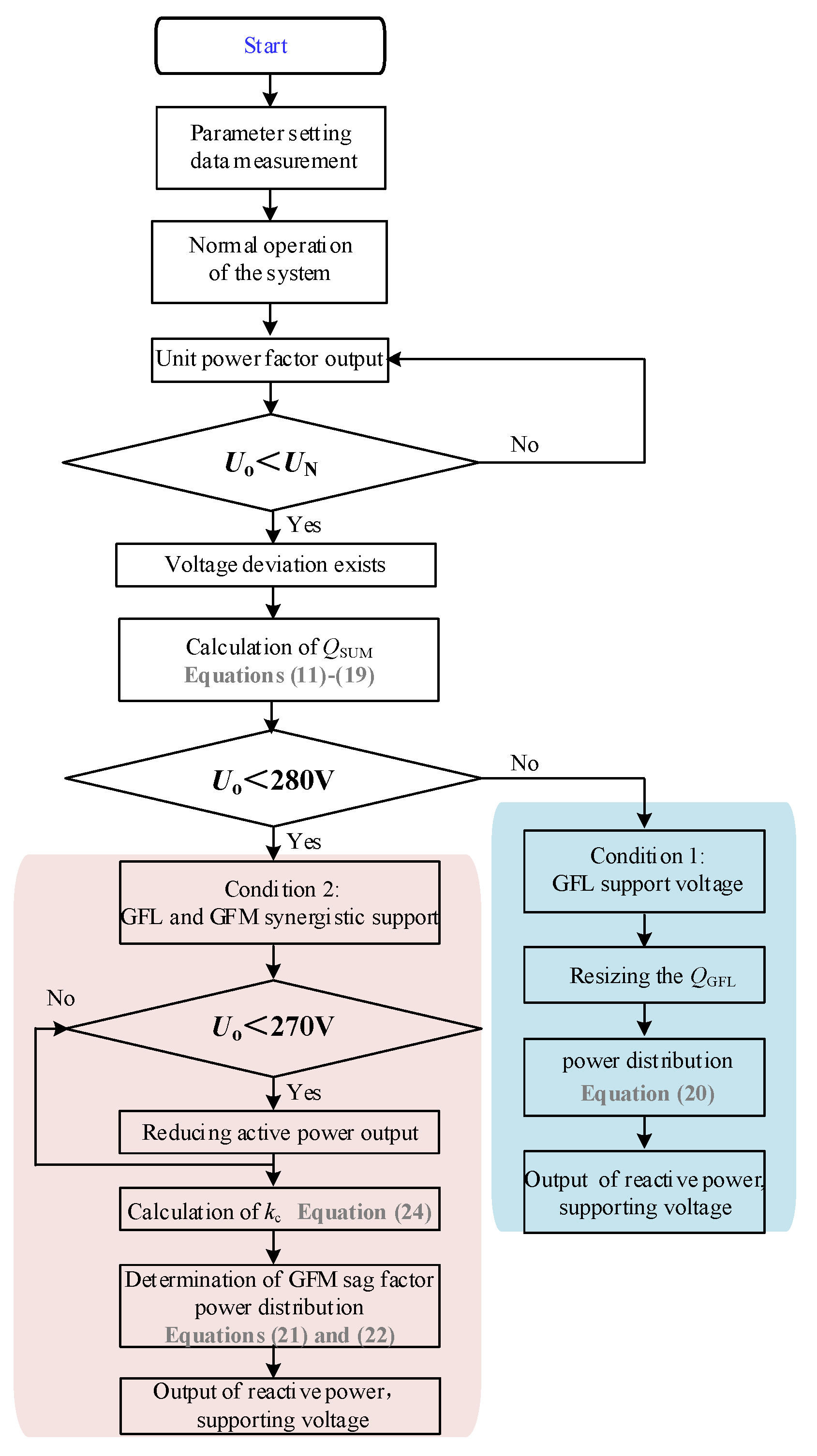
4. Cooperative Control Strategy for Voltage Support

4.1. Power Transmission Characteristics of the Parallel System

The GFL inverter and the GFM inverter both output power to the grid at the PCC. The rated active power of the GFL inverter is 40 kW. Generally, the capacity of a GFL inverter is 1.2 times of its rated active power. Therefore, the capacity of the GFL inverter in this paper is designed as 48 kVA. The rated active power of the GFM inverter is 10 kW. Similarly, the total capacity of the GFM inverter can be designed as 12 kVA. The capacity parameters of the MFGCIs are shown in

Table 1. Capacity of the inverters.

Symbol	Parameters	Value
SGFL	Rated capacity of GFL inverter	48 kVA
P1r	Reference active power of GFL inverter	40 kW
Q1r	Reference reactive power of GFL inverter	0 kVar
SGFM	Rated capacity of GFM inverter	12 kVA
P2r	Reference active power of GFM inverter	10 kW
Q2r	Reference reactive power of GFM inverter	0 kVar

, and other parameters are shown in

Table 2. Main circuit parameters.

Symbol	Parameters	Value
Vdc	Voltage on the DC side	800 V
Ugrid	Amplitude of grid voltage	311 V
L1	Filter inductor of GFL inverter	3 mH
L2	Filter inductor of GFM inverter	3 mH
R1	Equivalent resistance of L1	0.01 Ω
R2	Equivalent resistance of L2	0.01 Ω
Lg	Grid inductance	2.5 mH
Rg	Grid resistance	0.001 Ω
C1	Filter capacitor of GFL inverter	50 µF
C2	Filter capacitor of GFM inverter	50 µF
Rz1	Damping resistance of C1	4.5 Ω
Rz2	Damping resistance of C2	4.5 Ω
f0	Fundamental frequency of the grid	50 Hz
fsw	Switching frequency	10 kHz
Rnl	Resistance of non-linear loads	15 Ω
Cnl	Capacitance of non-linear loads	20 µF

and

Table 3. Main control parameters.

Symbol	Parameters	Value
Kpp	Proportionality coefficient for PLL	2.38
Kip	Integral coefficient for PLL	869
Kps	Proportionality coefficient for GFL power loop	0.0015
Kis	Integral coefficient for GFL power loop	1
kp	Droop coefficient of GFM active power loop	0.0002
kq	Droop coefficient of GFM reactive power loop	0.03

.

The output power of both the GFL and GFM inverters is calculated under the dq frame and the calculation expressions are shown in (12) and (13), respectively.

$$\left\{\begin{array}{l}{P}_{\mathrm{GFL}}={\displaystyle \frac{3}{2}}\left(U_{\mathrm{pl}d}{I}_{\mathrm{ll}d}+U_{\mathrm{pl}q}{I}_{\mathrm{ll}q}\right)\\ Q_{\mathrm{GFL}}={\displaystyle \frac{3}{2}}\left(U_{\mathrm{pl}q}{I}_{\mathrm{ll}d}-U_{\mathrm{pl}d}{I}_{\mathrm{ll}q}\right)\end{array}\right.$$

(12)

$$\left\{\begin{array}{l}{P}_{\mathrm{GFM}}={\displaystyle \frac{3}{2}}\left(U_{\mathrm{p}2d}{I}_{\mathrm{l}2d}+U_{\mathrm{p}2q}{I}_{\mathrm{l}2q}\right)\\ Q_{\mathrm{GFM}}={\displaystyle \frac{3}{2}}\left(U_{\mathrm{p}2q}{I}_{\mathrm{l}2d}-U_{\mathrm{p}2d}{I}_{\mathrm{l}2q}\right)\end{array}\right.$$

(13)

The sum of the GFL and GFM inverter output power is the total power output from the PCC to the grid:

$$\left\{\begin{array}{l}{P}_{\mathrm{SUM}}=P_{\mathrm{GFM}}+P_{\mathrm{GFL}}\\ Q_{\mathrm{SUM}}=Q_{\mathrm{GFM}}+Q_{\mathrm{GFL}}\end{array}\right.$$

(14)

The two inverters are connected to the grid through grid impedance. The power circuit relation is shown in (15).

$$\left[\begin{array}{c}{U}_{\mathrm{o}d}\\ U_{\mathrm{o}q}\end{array}\right]=\left[\begin{array}{cc}{L}_{\mathrm{g}}s+R_{\mathrm{g}}& -{\omega }_0{L}_{\mathrm{g}}\\ {\omega }_0{L}_{\mathrm{g}}& L_{\mathrm{g}}s+R_{\mathrm{g}}\end{array}\right]\left[\begin{array}{c}{I}_{\mathrm{g}d}\\ I_{\mathrm{g}q}\end{array}\right]+\left[\begin{array}{c}{U}_{\mathrm{grid}d}\\ U_{\mathrm{grid}q}\end{array}\right]$$

(15)

In the control loop, the d-axis coincides with the voltage vector. Therefore, the q-axis voltage component is 0, i.e., U_oq = 0. The expression for the output power of the PCC can be rewritten as:

$$\left\{\begin{array}{l}{P}_{\mathrm{SUM}}={\displaystyle \frac{3}{2}}\left(U_{\mathrm{o}d}{I}_{\mathrm{g}d}\right)\\ Q_{\mathrm{SUM}}={\displaystyle \frac{3}{2}}\left(-U_{\mathrm{o}d}{I}_{\mathrm{g}q}\right)\end{array}\right.$$

(16)

When the circuit parameters and total active power output remain constant, the relationship curve between U_o and U_grid can be obtained according to (15).

As illustrated in Figure 7, U_o decreases as U_grid drops. At P_SUM = 50 kW, U_o is lower than the rated value due to the voltage deviation resulting from grid impedance. The key of cooperative voltage support in MFGCIs is the sharing of reactive capacity. Therefore, the equation between U_o and the total output reactive power needs to be established. Combining (15) with (16) yields:

$$\left\{\begin{array}{l}{U}_{\mathrm{grid}d}=U_{\mathrm{o}d}-{\displaystyle \frac{\frac{2}{3}{R}_{\mathrm{g}}{P}_{\mathrm{SUM}}}{U_{\mathrm{o}d}}}-{\displaystyle \frac{\frac{2}{3}{\omega }_0{L}_{\mathrm{g}}{Q}_{\mathrm{SUM}}}{U_{\mathrm{o}d}}}\\ U_{\mathrm{grid}q}=-{\displaystyle \frac{\frac{2}{3}{\omega }_0{L}_{\mathrm{g}}{P}_{\mathrm{SUM}}}{U_{\mathrm{o}d}}}+{\displaystyle \frac{\frac{2}{3}{R}_{\mathrm{g}}{Q}_{\mathrm{SUM}}}{U_{\mathrm{o}d}}}\end{array}\right.$$

(17)

The relationship between the grid voltage magnitude and its dq-axis component satisfies:

$$U_{\mathrm{grid}d}^2+U_{\mathrm{grid}q}^2=|U_{\mathrm{grid}}{|}^2$$

(18)

Combining (17) and (18) can yield:

$$U_{\mathrm{o}d}^2+(2d_2-|U_{\mathrm{g}}{|}^2)U_{\mathrm{o}d}+({d_1}^2+{d_2}^2)=0$$

(19)

where

$$\left\{\begin{array}{l}{d}_1={\displaystyle \frac{2}{3}}(-{\omega }_0{L}_{\mathrm{g}}{P}_{\mathrm{SUM}}+R_{\mathrm{g}}{Q}_{\mathrm{SUM}})\\ d_2={\displaystyle \frac{2}{3}}(-{\omega }_0{L}_{\mathrm{g}}{Q}_{\mathrm{SUM}}-R_{\mathrm{g}}{P}_{\mathrm{SUM}})\end{array}\right.$$

Based on (19), U_o can be solved with the given U_grid. In Figure 8, the range of the total output reactive power is from 0 to 40 kVar, and the U_grid fluctuates in the range 0.85~1.0 pu. The supporting effect of the injected Q_SUM on U_o at varying levels of voltage drop can be observed, as illustrated in Figure 8.

In Figure 8, the X-axis is the injected reactive power, the Y-axis is the grid voltage, and the Z-axis is the U_o under different reactive power values.

The obtained results can directly evaluate the improvement effect of injecting the specified reactive power on U_o under different U_grid drop degrees. In Figure 8, the required reactive power raising U_o to the specific range can also be visually analyzed, which avoids repetitive analysis. As can be seen from points A₁ and A₂, the reactive power required for supporting U_o to 311.2 V is 19 kVar when U_grid drops to 290 V. When U_grid drops to 276 V, the required reactive power for supporting U_o to 310 V is 27.5 kVar. To simplify the analysis, the variation in grid impedance is ignored in this paper. Once grid impedance is determined, the reactive power to raise the voltage to the target value can be obtained.

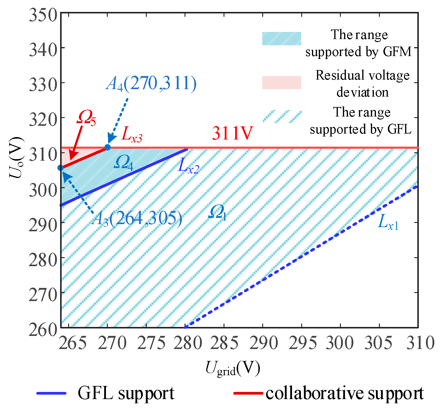
4.2. Analysis of Voltage Support Conditions in the Parallel System

In addition to harmonic suppression, MFGCIs can also have auxiliary function for voltage support. According to the capacity of MFGCIs, the parallel system involved in the voltage support includes two conditions. The first is that the GFL inverter supports the voltage independently. The second is that the GFL and GFM inverters support the voltage in concert. To simplify the analysis, only the symmetric voltage drop is considered in this paper, and the fluctuation range of U_grid is 0.85 pu~1 pu.

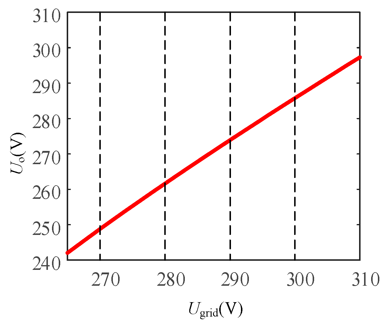
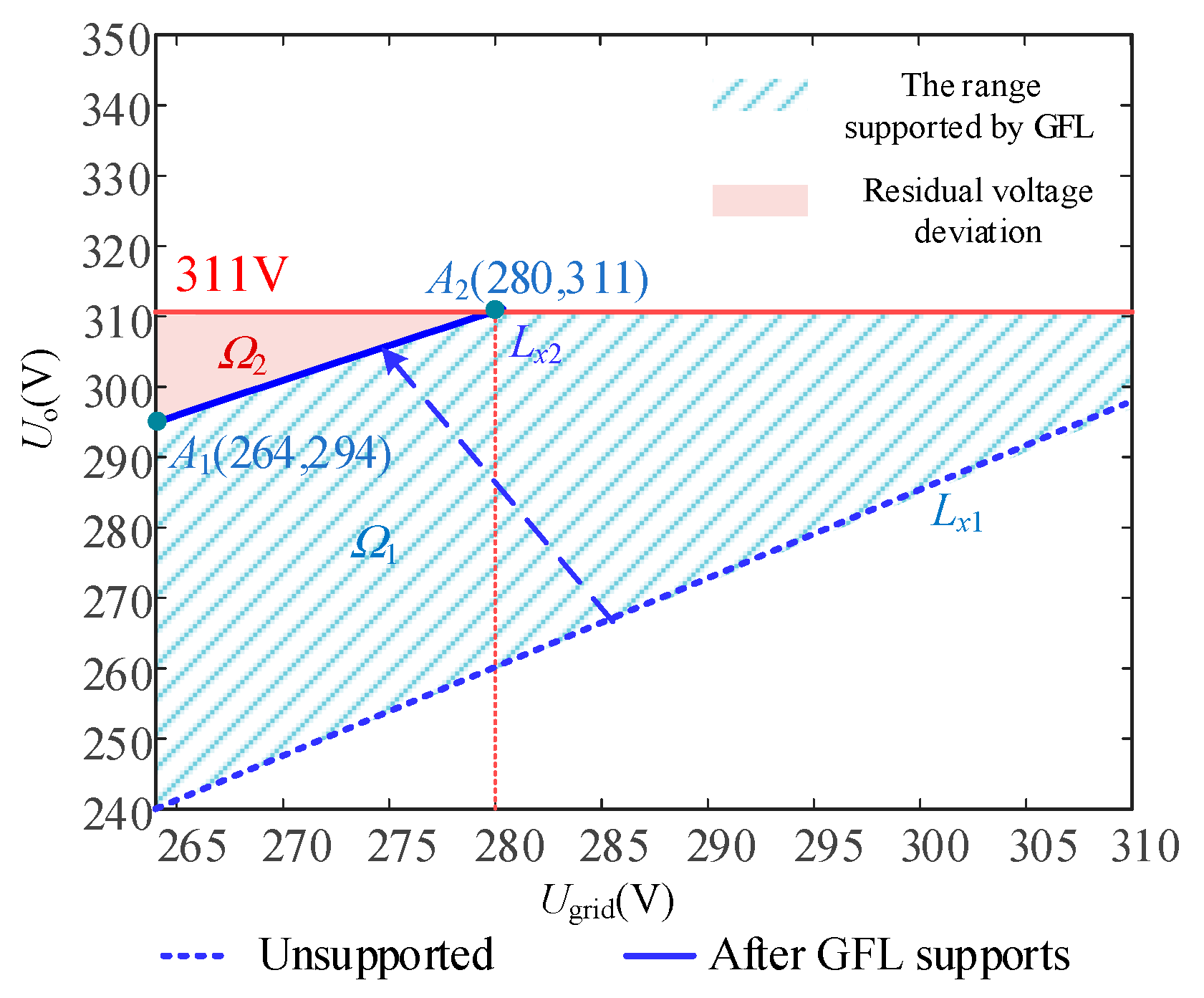
4.2.1. Operating Condition Where Only the GFL Inverter Supports Voltage

Under normal operation conditions, the GFL inverter and the GFM inverter only output active power. The active and reactive commands of the GFL inverter are 40 kW/0 Var and the active and reactive commands of the GFM inverter are 10 kW/0 Var.

When the grid voltage drops, the GFL inverter will adjust the output reactive power. At this time, only the GFL inverter supports voltage, and the power allocation is shown in (20).

Figure 9 shows the voltage support results of the GFL inverter. L_x1 denotes the boundary of U_o when the GFL inverter is not supporting the voltage after a drop in U_grid. L_x2 is the boundary of U_o when the GFL inverter outputs maximum reactive power. As shown in Figure 9, region Ω₁ is the voltage deviation regulated by the GFL inverter. Region Ω₂ is the support voltage range of the GFL inverter when outputting the maximum reactive power. When the grid voltage is higher than 280 V, the GFL inverter alone is enough to support the voltage to the specified value.

$$\left\{\begin{array}{l}{P}_{\mathrm{GFL}}=P_{1\mathrm{r}}\\ Q_{\mathrm{GFL}}=Q_{\mathrm{SUM}}\\ P_{\mathrm{GFM}}=P_{2\mathrm{r}}\\ Q_{\mathrm{GFM}}=0\end{array}\right.$$

(20)

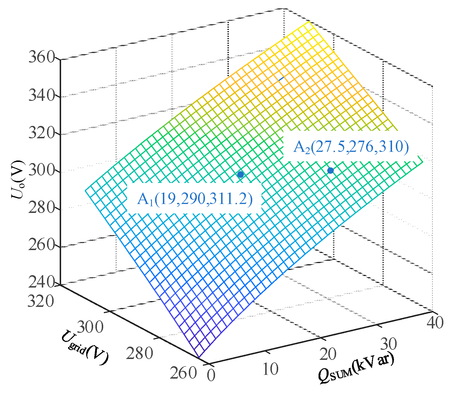
4.2.2. Operating Condition Where Both GFL and GFM Inverters Support Voltage

When the value of U_grid is lower than 280 V, the GFL inverter outputs the maximum reactive power, yet there is still a voltage deviation. As the GFL inverter capacity is insufficient, the GFM inverter also needs to support voltage. Then, the droop factor of the GFM inverter needs to be adjusted for auxiliary power compensation. Reactive power is shared between the GFL inverter and the GFM inverter according to the compensation factor. The compensation factor k_c is calculated as shown in (21).

$$k_c={\displaystyle \frac{S_{c1}}{S_{c1}+S_{c2}}}={\displaystyle \frac{\sqrt{S_{\mathrm{GFL}}-P_{1\mathrm{r}}^2}}{\sqrt{S_{\mathrm{GFL}}-P_{1\mathrm{r}}^2}+\sqrt{S_{\mathrm{GFM}}-P_{2\mathrm{r}}^2}}}$$

(21)

The power sharing relationship is shown in (22).

$$\left\{\begin{array}{l}{Q}_{\mathrm{GFL}}=k_{\mathrm{c}}{Q}_{\mathrm{SUM}}\\ Q_{\mathrm{GFM}}=\left(1-k_{\mathrm{c}}\right)Q_{\mathrm{SUM}}\end{array}\right.$$

(22)

where S_c1 and S_c2 are the remaining capacity of the GFL and GFM inverters, respectively.

After obtaining the compensated power of the GFM inverter, the reactive power–voltage droop factor is designed by [27]. The droop factor is designed according to the permissible voltage deviation of 1 V and the capacity of reactive power compensation as shown in (23). After adjusting the droop coefficient, based on the reactive power–voltage droop characteristic, the GFM outputs reactive power and actively supports the voltage.

$$k_q={\displaystyle \frac{V_{\mathrm{N}}-V_{\min }}{Q_{c2}-0}}$$

(23)

When the GFM inverter outputs reactive power, the voltage support range is shown in Figure 10. Regions Ω₁ and Ω₄ depict the range supported by the GFL inverter and GFM inverter, respectively. L_x3 is the boundary of U_o supported by the GFL inverter and GFM inverter in collaboration. The maximum support range for PCC voltage has been extended from 280 V to 270 V. However, due to the capacity constraint, the voltage at the PCC remains deviated when the voltage drop is more severe.

Furthermore, when the grid voltage drop degree is deeper, the active output can be reduced to provide more reactive power compensation capacity. After decreasing the active power, the total required reactive power needs to be recalculated according to (19). Then, the compensation coefficient is recalculated based on (24). According to the compensation coefficient, the reactive power allocated to the two inverters can be obtained.

$$k_c={\displaystyle \frac{S_{c1}}{S_{c1}+S_{c2}}}={\displaystyle \frac{\sqrt{S_{\mathrm{GFL}}-P_{\mathrm{GFL}}^2}}{\sqrt{S_{\mathrm{GFL}}-P_{\mathrm{GFL}}^2}+\sqrt{S_{\mathrm{GFL}}-P_{\mathrm{GFM}}^2}}}$$

(24)

In Equation (24), S_c1 and S_c2 represent the remaining capacity of the GFL and GFM inverters, respectively. The overall working flow of voltage support is shown in Figure 11.

5. Simulation Verification

5.1. Simulation Validation of Harmonic Suppression

A simulation model of the parallel system is constructed in Matlab 2022b/Simulink to verify the effectiveness of the proposed strategies. A three-phase bridge circuit is used as a typical non-linear load for verification. The relevant parameters are shown in Table 2 and Table 3. The diagrams used for simulation are shown in Figure 2. When the non-linear load is connected to the grid, the grid current contains harmonic currents. Before harmonic suppression, the magnitude of each order of harmonics is shown in Figure 12. After harmonic suppression, the magnitude of each order of harmonics is shown in Figure 13. As can be seen from the Figure 12, the magnitude of each harmonic is inversely proportional to the order of harmonics. Among them, the magnitude of the 5th, 7th, 11th, and 13th harmonics is higher, where the ratios account for 11.7%, 5.9%, 1.6%, and 2.9%, respectively.

Initially, a non-linear load is connected to the system and the active commands of the GFM inverter and GFL inverter are 10 kW and 30 kW, respectively. The reactive power reference value is 0 kVar for both inverters. At t = 0.3 s, the harmonic commands are added into both inverters. The inverters output harmonic components to compensate for non-linear load branch currents. At t = 0.4 s, the GFL inverter’s active power command is adjusted to 35 kW. The simulated waveforms are shown in Figure 14, Figure 15 and Figure 16.

As can be seen from Figure 12, before adding the harmonic suppression function, the three-phase grid current distortion is obvious, and the THD is 13.47%. After adding the harmonic suppression function, the power quality improvement effect is obvious, the grid current waveform is smoother, and the THD is reduced to 1.53%. And the magnitude of the 5th, 7th, 11th, and 13th harmonic currents is significantly reduced. It can be seen that the two inverters are distorted due to the output harmonic currents, and the GFL inverter mainly outputs the 5th and 7th harmonics, while the GFM inverter mainly outputs the 11th and 13th harmonics, which verifies the effectiveness of the proposed apportionment control strategy.

5.2. Simulation Verification of Voltage Cooperative Support

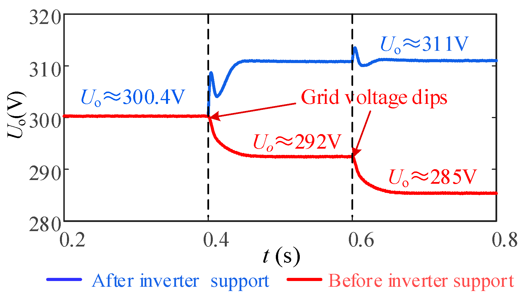
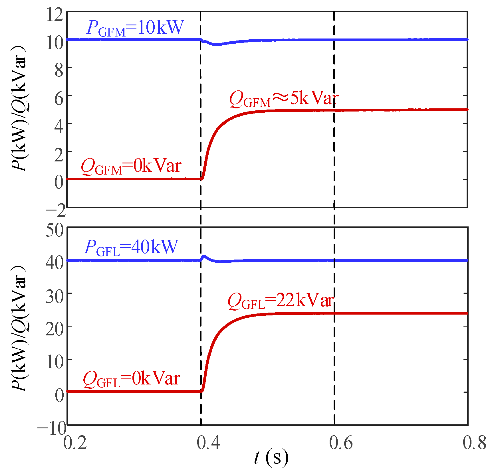
5.2.1. Condition Where Only the GFL Inverter Supports Voltage

The parallel system initially operates under unit power factor conditions. At t = 0–0.4 s, the active power of the GFL inverter and GFM inverter is 40 kW and 10 kW, respectively. At 0.4–0.6 s, the active power of the GFL inverter is reduced to 30 kW and the active power of the GFM inverter is reduced to 6 kW. Figure 17 and Figure 18 show the simulation results of the output power and PCC voltage under normal condition, respectively. The GFL and GFM inverters can quickly track the reference value when the active power changes suddenly. As can be seen from Figure 18, there is about 10 V voltage drop on grid impedance, and the voltage deviation decreases as the output power decreases.

The above simulation shows the output characteristics for normal conditions. Next, the strategy of single inverter support is verified. Initially, the system operates under unit power factor conditions with GFL and GFM active power command of 40 kW and 10 kW, respectively. At t = 0.4 s, the grid voltage drops and the GFL inverter outputs reactive power to support the voltage. At t = 0.6 s, U_o is also decreased to 285 V as U_grid drops to 290 V. According to Figure 8, the required total reactive power is 19 kVar, which is less than the maximum reactive capacity of the GFL inverter. Therefore, only the GFL inverter is needed to support the voltage. The results of the output power change and the PCC voltage before and after support are shown in Figure 19 and Figure 20.

As can be seen in Figure 20, U_o is about 292 V when U_grid drops to 300 V, and there is a large voltage deviation. After the GFL inverter outputs 12.7 kVar reactive power, U_o increases to near 311 V. As U_grid continues to drop, the value of U_o is about 292 V without the voltage support control. An accurate support of U_o can be achieved by increasing the reactive power output of the GFL inverter to 19 kVar.

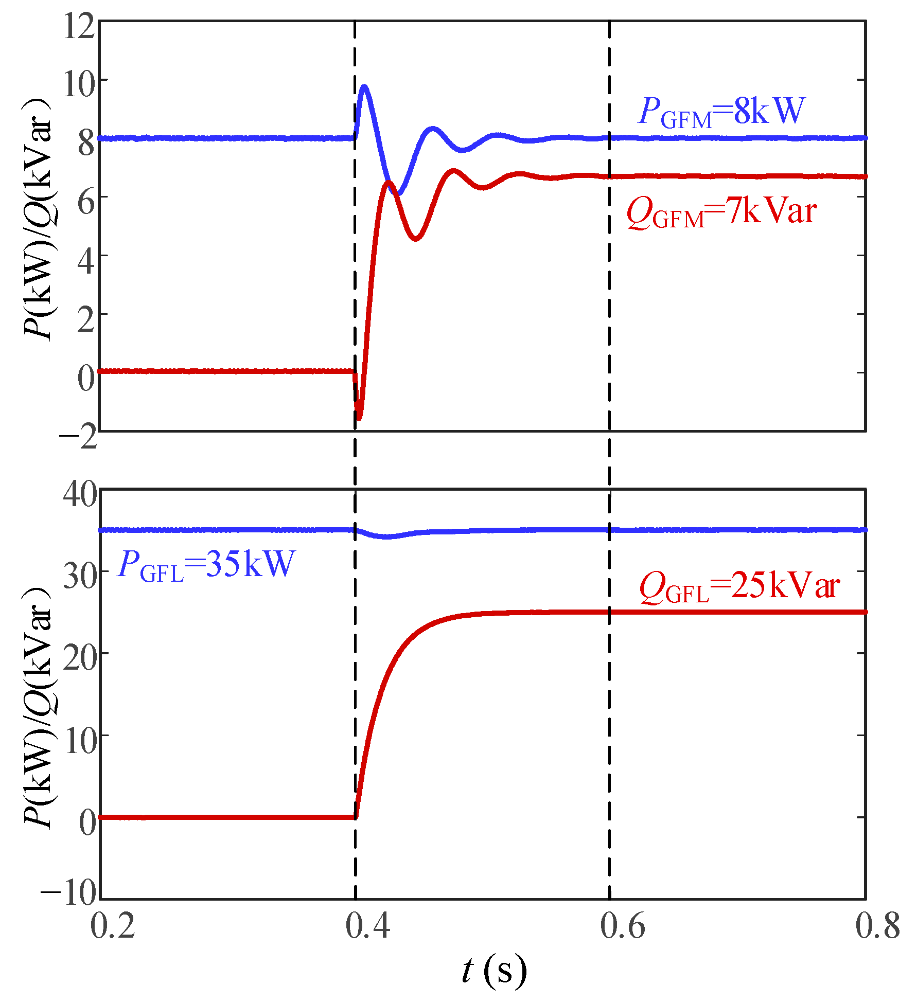
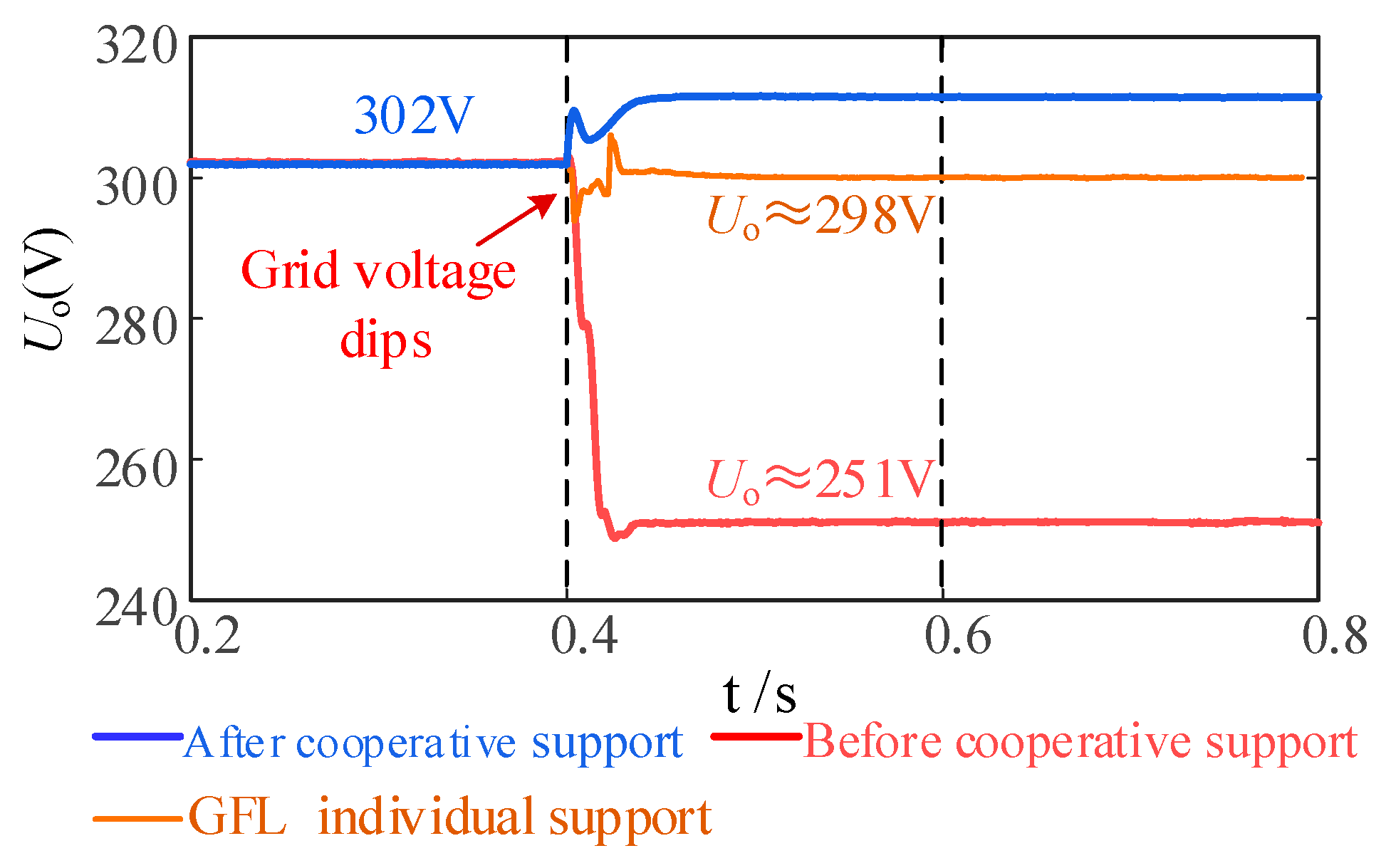
5.2.2. Conditions Where Voltage Is Supported by GFL and GFM Inverters in Concert

(1) When U_grid drops to 276 V, the required total reactive power reaches 27.5 kVar, which needs to be supported by the two types of inverters. According to (22), the compensation coefficient is 0.8 when the active command is constant. According to the power allocation in (23), the GFM and GFL inverters need to output 22 kVar and 5.5 kVar, respectively. The results of output power variation and support for U_o are shown in Figure 21 and Figure 22, respectively. From the figures, it can be seen that without support, U_o decreases to 259 V. When only the GFL inverter is considered for voltage support, U_o is about 307 V and there is still a voltage deviation. After the synergistic support of the GFL and GFM inverters, U_o is restored to near the rated voltage. Cooperative support can improve the voltage support effect.

(2) When U_grid is dropped to 266 V, the output active powers of the two inverters are reduced to 8 kW and 35 kW to improve the support capacities. The required reactive capacity is recalculated to be 32 kVar based on (19) and the compensation factor is calculated to be 0.214 according to (24). The reactive powers shared by the GFM and GFL inverters are 6.8 kVar and 25.2 kVar, respectively. Thus, the reactive power command and the corresponding droop coefficient are obtained. The simulation results are shown in Figure 23 and Figure 24. From the figures, it can be seen that without support, Uo decreases to 251 V. When the GFL inverter supports voltage individually, U_o is about 298 V, and there is still a large voltage deviation. After the GFL and GFM inverters support voltage synergistically, U_o is restored to the rated voltage. The support effect after synergistic control is significantly better than that of the GFL inverter support, which verifies the correctness of the proposed strategy.

As can be seen, the output power approaches the obtained calculations. It is clear that U_o decreases and power quality deteriorates as U_grid drops. After supporting the voltage, the PCC voltage deviation is reduced. The simulation results of the required compensated power after voltage drop are in agreement with the theoretical analysis. The support effect after the synergistic control of the GFL and GFM inverters is significantly better than that of the GFL inverter’s individual support, which verifies the correctness of the proposed strategy. The above simulation results verify the effectiveness of the proposed cooperative control strategy.

6. Experimental Verification

The relevant parameters are shown in Table 2 and Table 3. The diagrams used for the experiment are shown in Figure 2. In order to verify the effectiveness of the proposed harmonic suppression and voltage support strategies, relevant models are constructed for experimental verification.

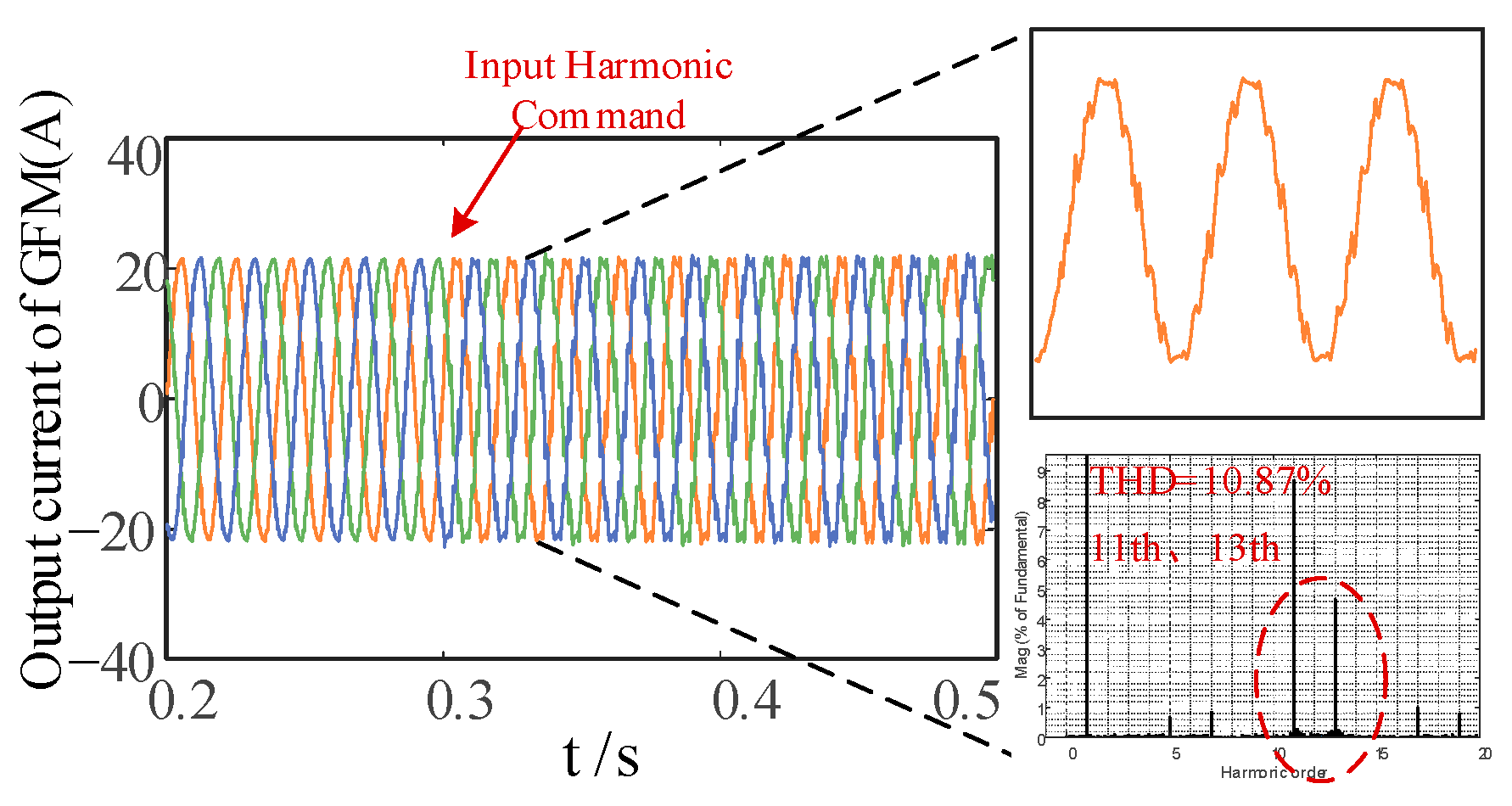
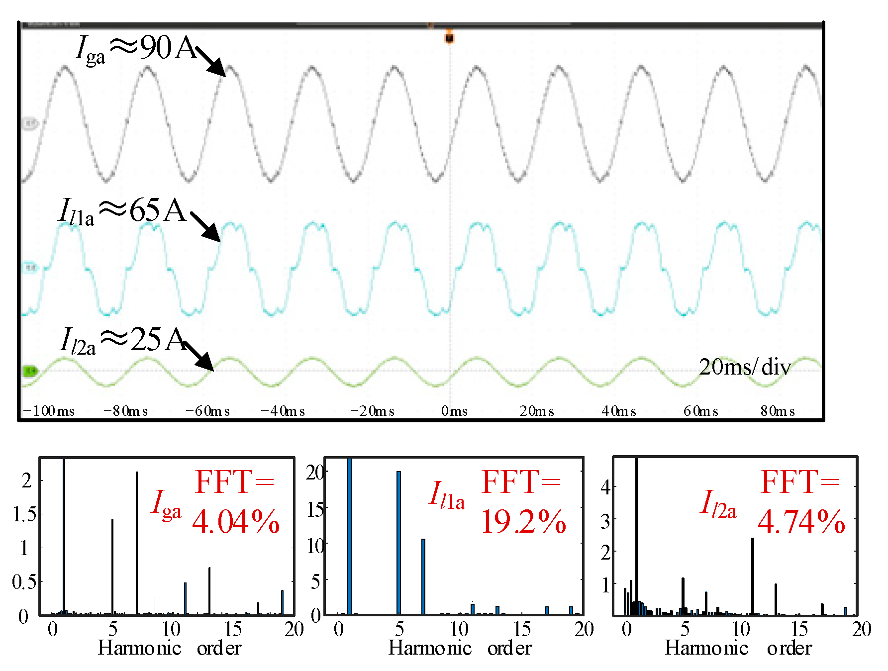
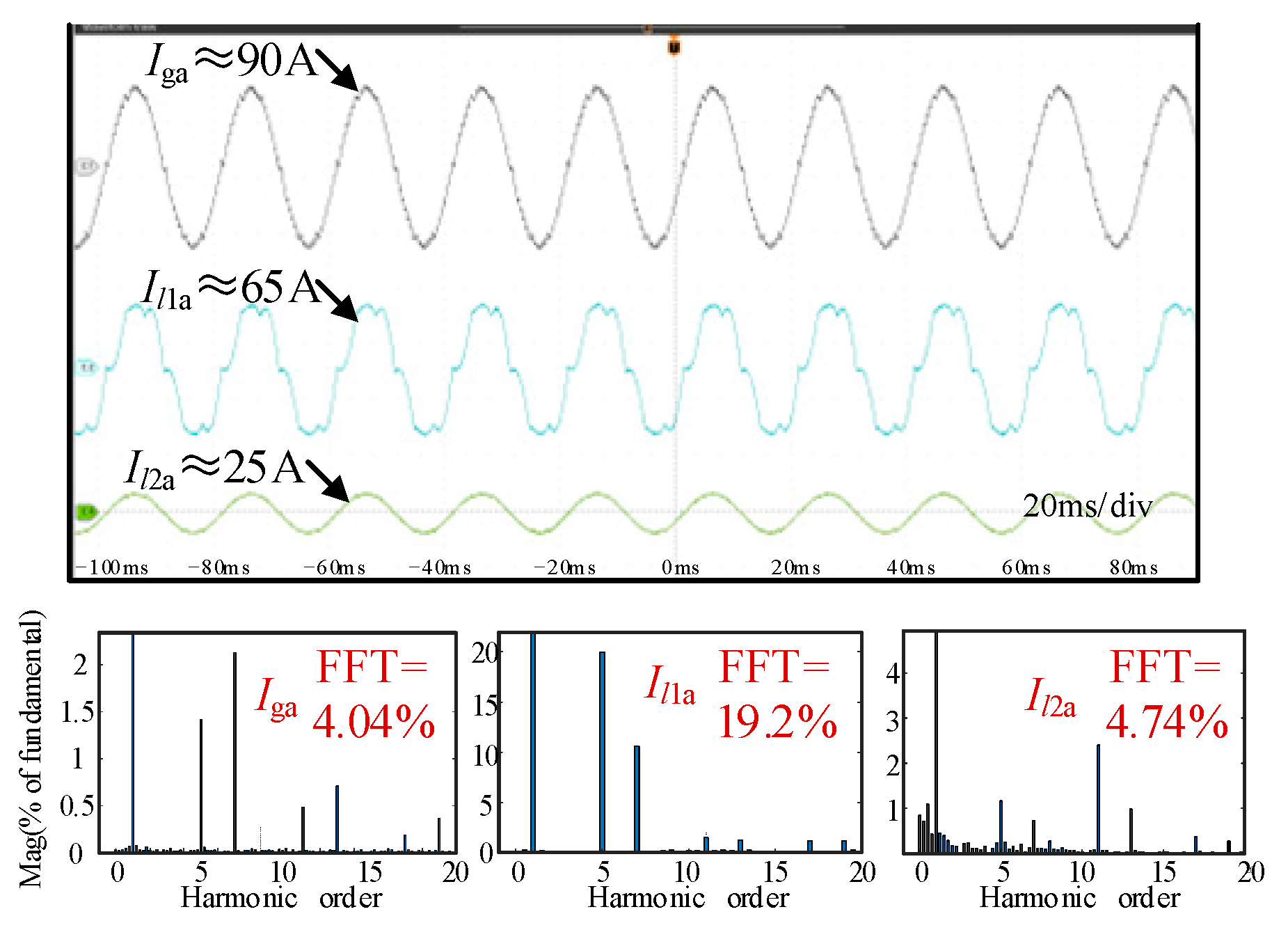
6.1. Experimental Verification of Harmonic Suppression

Figure 25 shows the experimental waveforms of A-phase grid current (I_ga), A-phase GFL inverter current (I_l1a), and A-phase GFM inverter current (I_l2a) without harmonic suppression. It can be seen from the figure that due to the presence of non-linear loads in the system, the THD of the grid current is about 13.3%, which is dominated by the 5th, 7th, 11th, and 13th harmonics. The THD of the currents of both the GFL and the GFM inverter is below 5%.

Figure 26 shows the experimental waveforms of the A-phase grid current, the A-phase GFL inverter current, and the A-phase GFM inverter current after performing harmonic suppression. From the figure, it can be seen that the GFL inverter mainly outputs the 5th and 7th harmonics and the GFM inverter mainly outputs the 11th and 13th harmonics. The THD of the grid current is reduced to 4.04% after harmonic compensation for both inverters. The magnitude of the 5th, 7th, 11th, and 13th harmonics of the grid current is reduced. Experimental waveforms verify the effectiveness of the proposed harmonic suppression strategy.

6.2. Experimental Verification of Voltage Cooperative Support

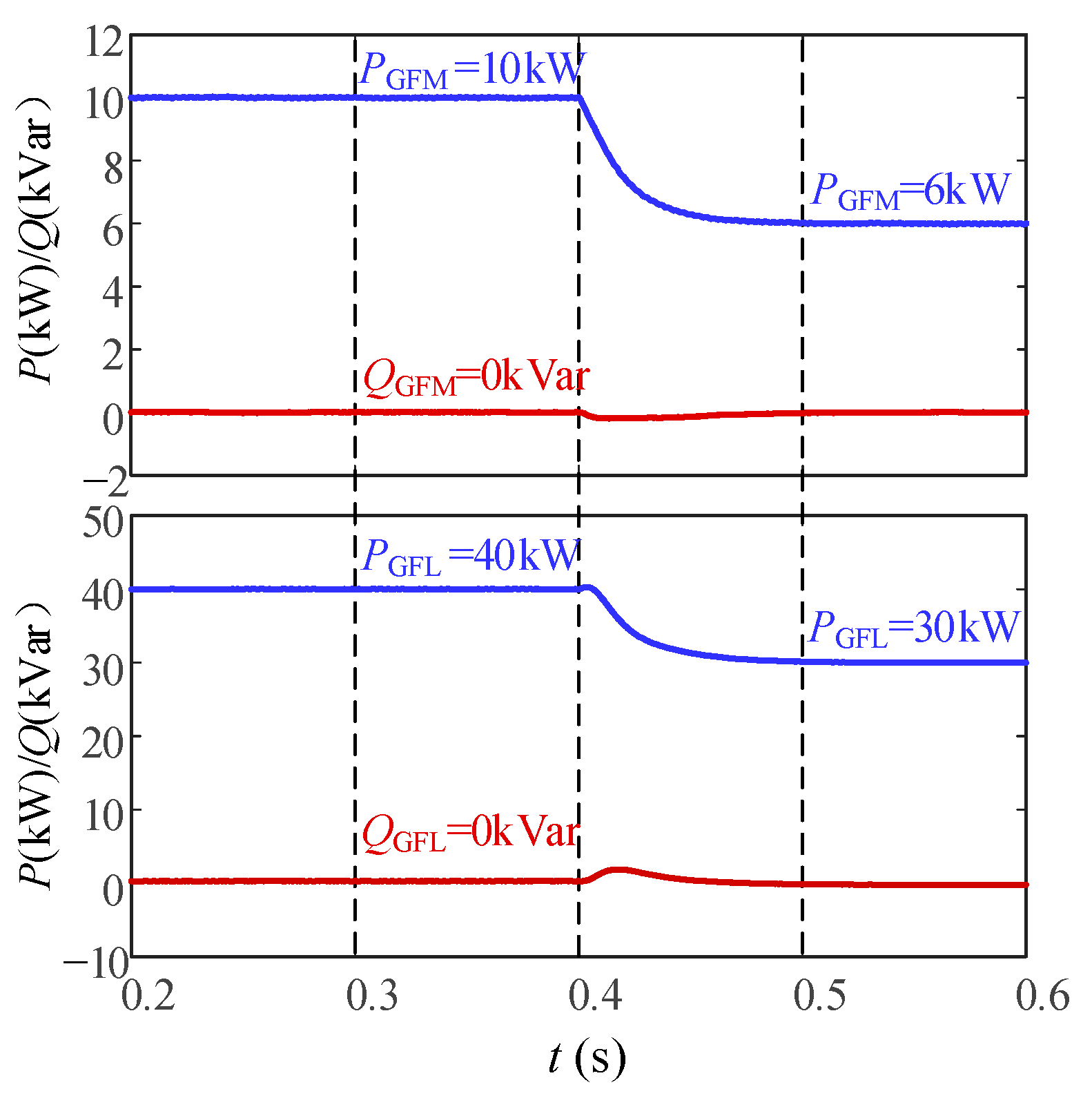
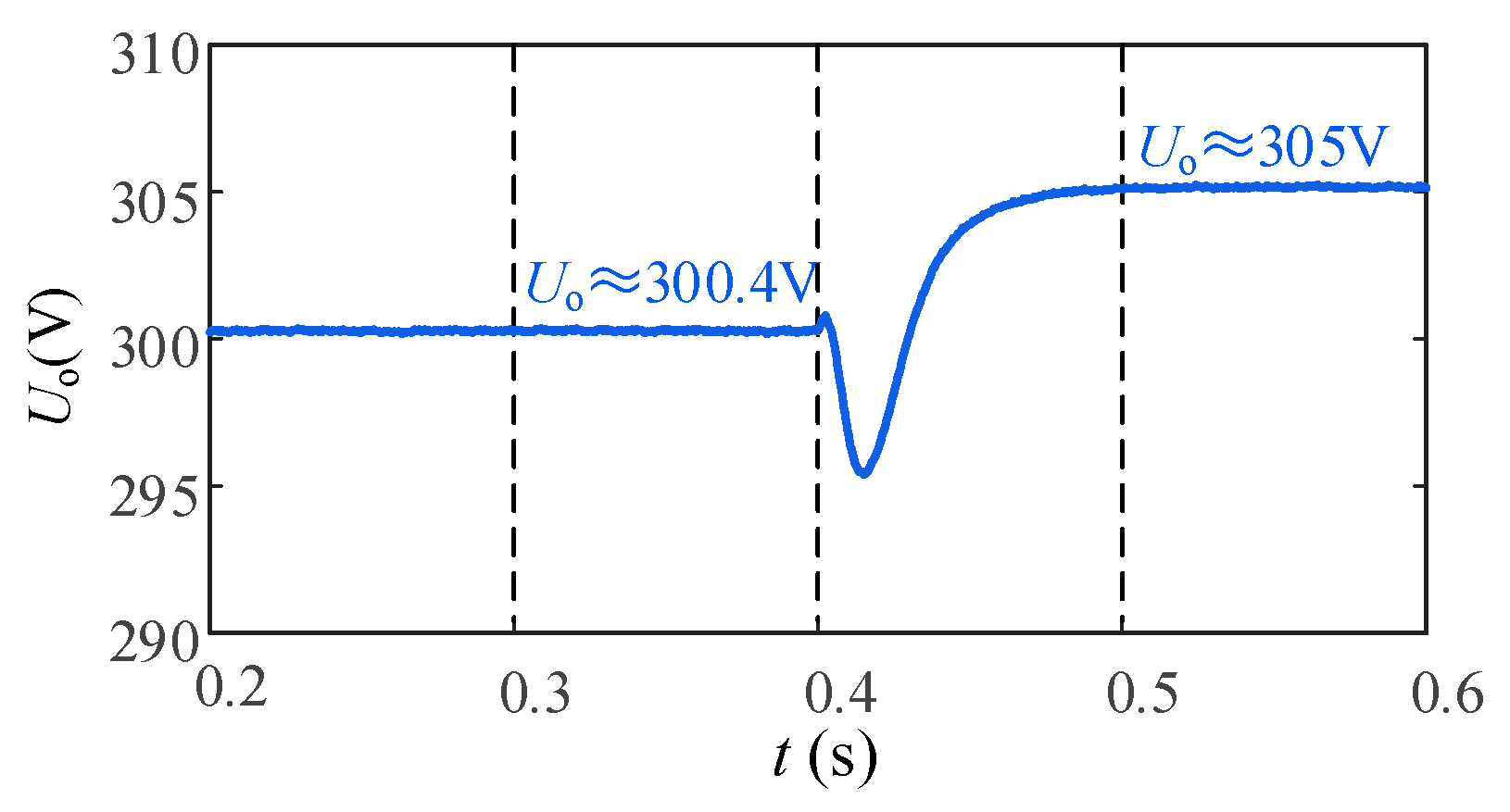
6.2.1. Working Condition Where Only the GFL Inverter Supports Voltage

The experimental results of the GFL inverter individually supporting voltage are shown in Figure 27. From the obtained experimental results, it can be seen that before the grid voltage drops, U_o is about 300 V due to the voltage drop across grid impedance. After the grid voltage dips, U_o decreases to 285 V. According to the previous analysis, U_o is supported by the GFL individually in this working condition. After the GFL inverter outputs 20 kVar of reactive power, U_o is supported close to its rated value.

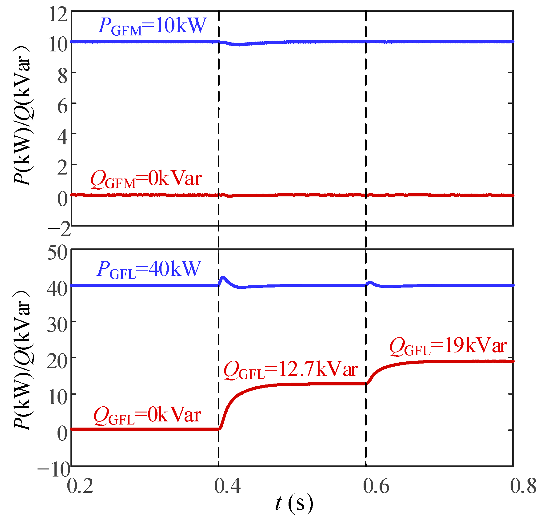
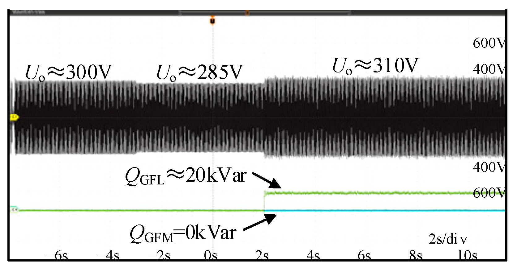
6.2.2. Condition Where Voltage Is Supported by GFL and GFM Inverters in Concert

The experimental results of voltage support by the GFL and GFM inverters in concert are shown in Figure 28. From the obtained experimental results, it can be seen that before the grid voltage drops, U_o is about 300 V. After the grid voltage dips, U_o decreases to 250 V. According to the previous analysis, U_o is supported by the GFL inverter and the GFM inverter cooperatively. The control strategy is engaged after the grid voltage dips for 5 s. After the GFL inverter and GFM inverter output 20 kVar and 7 kVar reactive power, respectively, U_o is supported near the rated voltage. The experimental results verify the effectiveness of the proposed voltage support strategy.

7. Conclusions

This paper proposes a collaborative control method of power quality based on the heterogeneous inverter parallel system, and the main work and conclusions are as follows:

• With the introduction of large-scale renewable energy sources, power electronics has become an important feature of modern power systems. GFL and GFM inverters in parallel are the trend of the future due to their ability to satisfy both customer and system requirements in terms of voltage/frequency regulation and power quality.
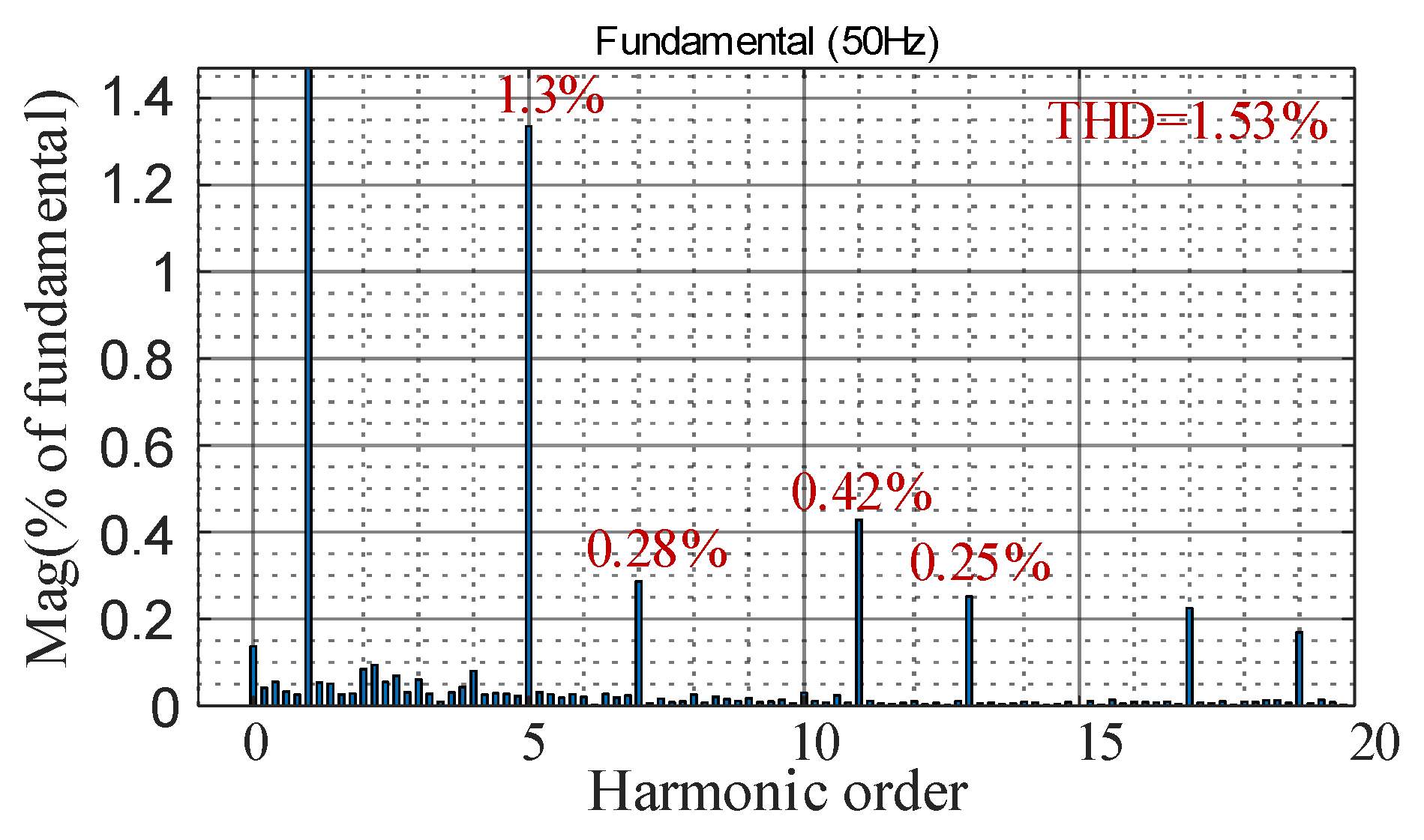
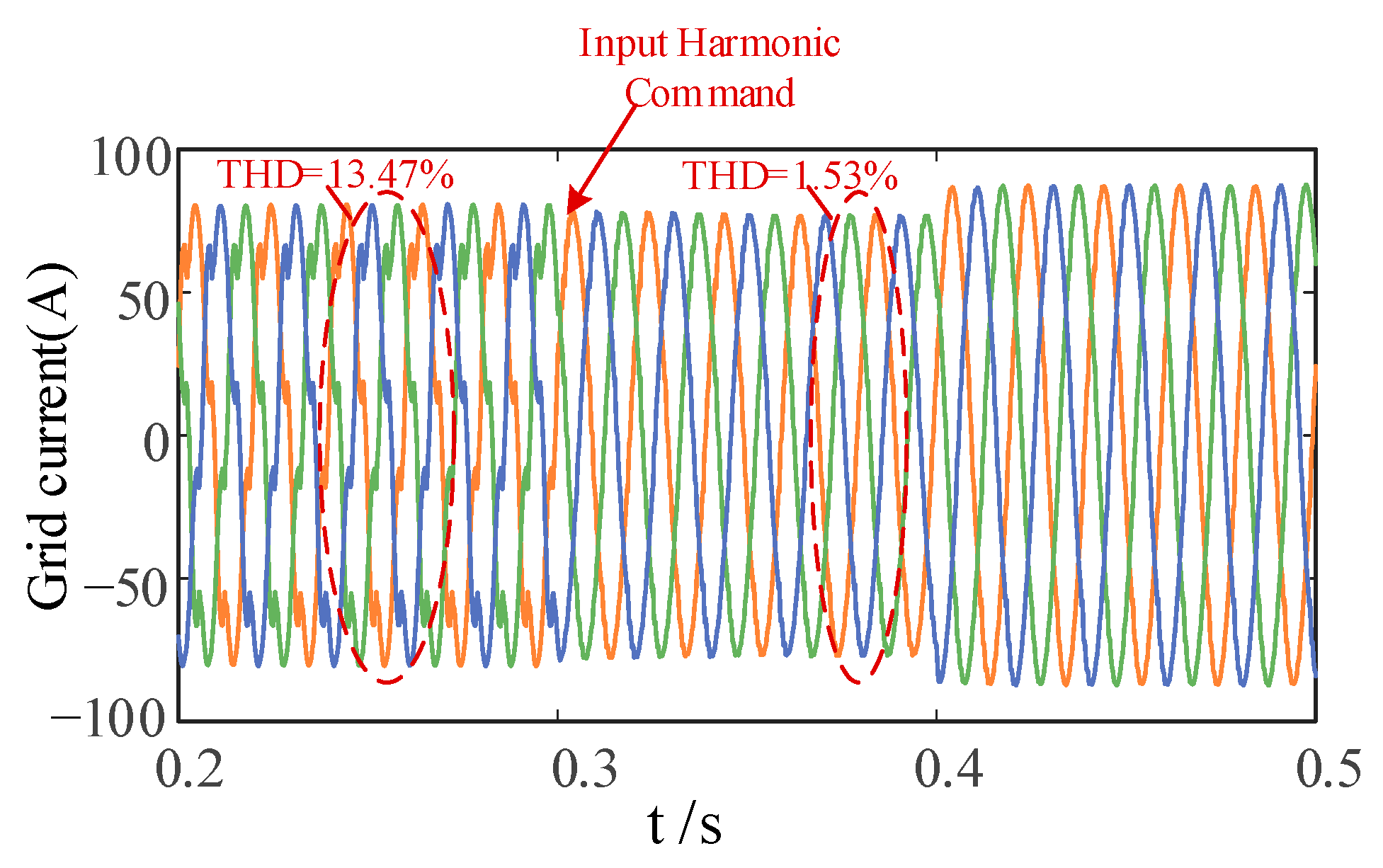
• In this paper, the characteristics of GFL and GFM inverters are fully utilized. While ensuring power transmission, the remaining capacity is fully utilized to carry out the auxiliary control of power quality problems such as harmonic problems and voltage deviation. A harmonic allocation control strategy based on QRC is proposed, which can effectively control and allocate the 5th, 7th, 11th, and 13th harmonics. A coordinated control strategy of voltage support is proposed, which can better realize the accurate support of PCC voltage.
• Through simulation verification, the GFL inverter outputs the 5th and 7th harmonics, and the GFM inverter outputs the 11th and 13th harmonics. The THD of the grid current can be reduced from 13.47 to 1.53%. When the grid voltage drops to 251 V, there is still a voltage deviation of 13 V when the GFL inverter supports voltage alone, and after coordinated control, the PCC voltage can be accurately supported near the rated voltage. Although this paper analyzes specific scenarios, the proposed method has the value of generalized application.

References

1. He, J.; Li, Y.W.; Wang, R.; Wang, C. A measurement method to solve a problem of using DG interfacing converters for selective load harmonic filtering. IEEE Trans. Power Electron. 2016, 31, 1852–1856. [Google Scholar] [CrossRef]
2. de Jesus, V.M.R.; Cupertino, A.F.; Xavier, L.S.; Pereira, H.A.; Mendes, V.F. Comparison of MPPT strategies in three-phase photovoltaic inverters applied for harmonic compensation. IEEE Trans. Ind. Appl. 2019, 55, 5141–5152. [Google Scholar] [CrossRef]
3. Osorio, F.; Mantilla, M.A.; Rey, J.M.; Petit, J.F. A flexible control strategy for multi-functional pv inverters with load compensation capabilities considering current limitations and unbalanced load conditions. Energies 2024, 17, 4218. [Google Scholar] [CrossRef]
4. Kaur, S.; Dwivedi, B. Power quality issues and their mitigation techniques in microgrid system-a review. In Proceedings of the 7th India International Conference on Power Electronics (IICPE), Patiala, India, 17–19 November 2016; p. 1. [Google Scholar]
5. Wei, Y.; Wang, J.; Li, N. An analysis of the influence of grid-connected renewable energy on power quality of power grids. Power Syst. Clean Energy 2022, 38, 108–114. [Google Scholar]
6. Wang, J.; Sun, K.; Wu, H.; Zhu, J.; Xing, Y.; Li, Y. Hybrid connected unified power quality conditioner integrating distributed generation with reduced power capacity and enhanced conversion efficiency. IEEE Trans. Ind. Electron. 2020, 68, 12340–12352. [Google Scholar] [CrossRef]
7. Acuna, P.; Moran, L.; Rivera, M.; Dixon, J.; Rodriguez, J. Improved active power filter performance for renewable power generation systems. IEEE Trans. Power Electron. 2013, 29, 687–694. [Google Scholar] [CrossRef]
8. Zhang, K.; Wang, L.; Pang, Y.; Liao, S.; Yang, X.; Wong, M.C. Power selective control with fault tolerance of multifunctional inverter for active power injection and power quality compensation. IEEE Trans. Ind. Electron. 2022, 70, 4309–4319. [Google Scholar] [CrossRef]
9. Ali, Z.; Christofides, N.; Hadjidemetriou, L.; Kyriakides, E. Multi-functional distributed generation control scheme for improving the grid power quality. IET Power Electron. 2019, 12, 30–43. [Google Scholar] [CrossRef]
10. Zeng, Z.; Yang, H.; Zhao, R.; Cheng, C. Topologies and control strategies of multi-functional grid-connected inverters for power quality enhancement: A comprehensive review. Renew. Sustain. Energy Rev. 2013, 24, 223–270. [Google Scholar] [CrossRef]
11. Pranith, S.; Kumar, S.; Singh, B.; Bhatti, T.S. Multimode operation of PV-battery system with renewable intermittency smoothening and enhanced power quality. IET Renew. Power Gener. 2019, 13, 887–897. [Google Scholar] [CrossRef]
12. Wang, J.; Sun, K.; Wu, H.; Zhang, L.; Zhu, J.; Xing, Y. Quasi-two-stage multifunctional photovoltaic inverter with power quality control and enhanced conversion efficiency. IEEE Trans. Power Electron. 2019, 35, 7073–7085. [Google Scholar] [CrossRef]
13. Akagi, H.; Watanabe, E.H.; Aredes, M. Instantaneous power theory and applications to power conditioning. In Instantaneous Power Theory and Applications to Power Conditioning; John Wiley & Sons: Hoboken, NJ, USA, 2017. [Google Scholar]
14. Simões, M.G.; Busarello, T.D.C.; Bubshait, A.S.; Harirchi, F.; Pomilio, J.A.; Blaabjerg, F. Interactive smart battery storage for a PV and wind hybrid energy management control based on conservative power theory. Int. J. Control 2016, 89, 850–870. [Google Scholar] [CrossRef]
15. Paredes, H.K.M.; Rodrigues, D.T.; Cebrian, J.C.; Bonaldo, J.P. CPT-based multi-objective strategy for power quality enhancement in three-phase three-wire systems under distorted and unbalanced voltage conditions. IEEE Access 2021, 9, 53078–53095. [Google Scholar] [CrossRef]
16. Li, Z.; Wang, Y.; Cui, B. An improved adaptive harmonic detection algorithm. In Proceedings of the 24th International Conference on Automation and Computing (ICAC), Newcastle Upon Tyne, UK, 6–7 September 2018. [Google Scholar]
17. Choi, W.; Lee, W.; Han, D.; Sarlioglu, B. New configuration of multifunctional grid-connected inverter to improve both current-based and voltage-based power quality. IEEE Trans. Ind. Appl. 2018, 54, 6374–6382. [Google Scholar] [CrossRef]
18. Zhang, X.; Spencer, J.W.; Guerrero, J.M. Small-signal modeling of digitally controlled grid-connected inverters with LCL filters. IEEE Trans. Ind. Electron. 2012, 60, 3752–3765. [Google Scholar] [CrossRef]
19. Alves, A.G.P.; Rolim, L.G.B.; da Silva Dias, R.F.; dos Santos Ramos, J. Analysis of grid-connected VSCs subject to voltage harmonic disturbances: Prediction and design tool of resonant controllers. IEEE Trans. Energy Convers. 2023, 38, 239–249. [Google Scholar] [CrossRef]
20. Golestan, S.; Ebrahimzadeh, E.; Guerrero, J.M.; Vasquez, J.C. An adaptive resonant regulator for single-phase grid-tied VSCs. IEEE Trans. Power Electron. 2018, 33, 1867–1873. [Google Scholar] [CrossRef]
21. Ramos, G.A.; Ruget, R.I.; Costa-Castelló, R. Robust repetitive control of power inverters for standalone operation in DG systems. IEEE Trans. Energy Convers. 2020, 35, 237–247. [Google Scholar] [CrossRef]
22. Qing, H.; Zhang, C.; Chai, X.; He, H.; Wang, X. Research on grid-connected harmonic current suppression of three-phase four-wire energy storage inverters. J. Power Electron. 2023, 23, 972–983. [Google Scholar] [CrossRef]
23. Teng, Y.; Deng, W.; Pei, W.; Li, Y.; Dingv, L.; Ye, H. Review on grid-forming converter control methods in high-proportion renewable energy power systems. Glob. Energy Interconnect. 2022, 5, 328–342. [Google Scholar] [CrossRef]
24. Li, Y.; Gu, Y.; Green, T.C. Revisiting grid-forming and grid-following inverters: A duality theory. IEEE Trans. Power Syst. 2022, 37, 4541–4554. [Google Scholar] [CrossRef]
25. Zhang, H.; Wang, W.; Lin, W.; Wen, J. Grid forming converters in renewable energy sources dominated power grid: Control strategy, stability, application, and challenges. J. Mod. Power Syst. Clean Energy 2021, 9, 1239–1256. [Google Scholar] [CrossRef]
26. Zhang, C.; Dou, X.; Wang, L.; Dong, Y.; Ji, Y. Distributed cooperative voltage control for grid-following and grid-forming distributed generators in islanded microgrids. IEEE Trans. Power Syst. 2022, 38, 589–602. [Google Scholar] [CrossRef]
27. Rosso, R.; Engelken, S.; Liserre, M. Robust stability investigation of the interactions among grid-forming and grid-following converters. IEEE J. Emerg. Sel. Top. Power Electron. 2019, 8, 991–1003. [Google Scholar] [CrossRef]
28. Cheng, H.; Shuai, Z.; Shen, C.; Liu, X.; Li, Z.; Shen, Z.J. Transient angle stability of paralleled synchronous and virtual synchronous generators in islanded microgrids. IEEE Trans. Power Electron. 2020, 35, 8751–8765. [Google Scholar] [CrossRef]
29. Shen, C.; Shuai, Z.; Shen, Y.; Peng, Y.; Liu, X.; Li, Z.; Shen, Z.J. Transient stability and current injection design of paralleled current-controlled VSCs and virtual synchronous generators. IEEE Trans. Smart Grid 2020, 12, 1118–1134. [Google Scholar] [CrossRef]
30. Pengyin, L.; Hui, L.; Linlin, W.; Yunhong, L.I.; Siqi, Y.U.; Xiaorong, X.I. Grid-following and grid-forming combined control and optimal configuration to satisfy oscillation constraints across whole operating region. Autom. Electr. Power Syst. 2024, 48, 139–146. [Google Scholar]
Figure 1. Topology of the inverters.
Energies 17 06226 g001
Figure 2. Structure and control strategy of parallel system.
Energies 17 06226 g002
Figure 3. Structure of PLL.
Energies 17 06226 g003
Figure 4. The droop control outer loop of GFM inverter.
Energies 17 06226 g004
Figure 5. Detection of harmonic current.
Energies 17 06226 g005
Figure 6. Parallel PI and QRC controller. (a) Current loop of GFL; (b) current loop of GFM.
Energies 17 06226 g006
Figure 7. The relationship curve between Ugrid and Uo.
Energies 17 06226 g007
Figure 8. The Uo variation surface under different reactive power values.
Energies 17 06226 g008
Figure 9. Uo boundary after voltage support with only GFL inverter.
Energies 17 06226 g009
Figure 10. The Uo boundary after coordinated support.
Energies 17 06226 g010
Figure 11. The overall working flow of the parallel system for voltage support.
Energies 17 06226 g011
Figure 12. The magnitude of each harmonic of the grid current before suppression.
Energies 17 06226 g012
Figure 13. The magnitude of each harmonic of the grid current after suppression.
Energies 17 06226 g013
Figure 14. The simulation waveform of the grid current.
Energies 17 06226 g014
Figure 15. The output current of the GFL inverter.
Energies 17 06226 g015
Figure 16. The output current of the GFM inverter.
Energies 17 06226 g016
Figure 17. Output power waveform under normal conditions.
Energies 17 06226 g017
Figure 18. Voltage amplitude of PCC under normal conditions.
Energies 17 06226 g018
Figure 19. Output power when only GFL inverter supports voltage.
Energies 17 06226 g019
Figure 20. The voltage support effect when only the GFL inverter is involved.
Energies 17 06226 g020
Figure 21. The output power of the GFM and GFL inverters when they support voltage in concert.
Energies 17 06226 g021
Figure 22. The voltage support effect of the GFM and GFL inverters is coordinated.
Energies 17 06226 g022
Figure 23. The voltage support effect in case of severe voltage drops.
Energies 17 06226 g023
Figure 24. The voltage support effect of the GFM and GFL inverters is coordinated.
Energies 17 06226 g024
Figure 25. Experimental waveforms before harmonic suppression.
Energies 17 06226 g025
Figure 26. Experimental waveforms after harmonic suppression.
Energies 17 06226 g026
Figure 27. Experimental waveforms supported by GFL inverter alone.
Energies 17 06226 g027
Figure 28. Experimental waveforms after synergistic support.
Energies 17 06226 g028