Article

Robustness-Based Evaluation of GHG Emissions and Energy Use at Neighborhood Level †

by
Roberta Moschetti
1,*,‡ and
Shabnam Homaei
2,‡
1
Department of Architecture, Materials and Structures, SINTEF Community, 7034 Trondheim, Norway
2
Department of Architectural Engineering, SINTEF Community, 0373 Oslo, Norway
*
Author to whom correspondence should be addressed.
This paper is an extended version of our paper published in Homaei, S.; Moschetti, R.; Clauss, J. Selection of the most high-performance and robust design for a zero-emission neighbourhood: Case study of Flytårnet area in Norway. In Proceedings of the Building Simulation 2023: 18th Conference of IBPSA, Shanghai, China, 4–6 September 2023.
These authors contributed equally to this work.
Energies 2024, 17(23), 6210; https://doi.org/10.3390/en17236210
Submission received: 4 October 2024 / Revised: 12 November 2024 / Accepted: 2 December 2024 / Published: 9 December 2024
(This article belongs to the Collection Feature Papers in Energy, Environment and Well-Being)

Abstract

:
Evaluating neighborhood performance is crucial for achieving long-term zero-carbon goals, enabling efficient energy, cost, and resource sharing among buildings. This task requires balancing multiple criteria and managing uncertainties, emphasizing the importance of performance robustness alongside high performance. This article introduces a flexible multi-criteria approach for evaluating neighborhood performance, focusing on greenhouse gas (GHG) emissions and energy use across different life cycle stages. Flytårnet, a Norwegian neighborhood with zero-emission ambitions, serves as a case study. The methodology incorporates the T-robust method, an established robustness-based approach, to select high-performance, resilient neighborhood designs under various uncertainties. Results indicate that when assessing buildings as key components and considering energy delivered during the operational phase, including photovoltaic generation, the supplied energy ranges from 25 to 80 kWh/m2/year. Over a 60-year period, life cycle GHG emissions span from 4 to 12 kg CO2-eq./m2/year, accounting for uncertainties and encompassing material production and replacement, as well as energy consumption and generation. However, the optimal design choice varies based on whether life cycle stages beyond the use stage are considered. This research provides valuable insights for decision-makers and designers seeking effective neighborhood designs in early-stage planning, considering diverse and conflicting performance criteria to achieve zero-emission goals.

1. Introduction

1.1. Background

Climate change mitigation initiatives are increasingly being implemented at local levels, with decision-makers, such as municipalities, needing effective tools to select appropriate policy interventions to tackle climate challenges [1]. Making decisions at larger scales, such as for neighborhoods, communities, and cities, is particularly complex due to the need to balance multiple conflicting performance criteria under conditions of uncertainty [2].
Similar to individual buildings, the performance of a neighborhood can be influenced by various uncertainties, such as operational unpredictability and external factors. It is therefore crucial to minimize the impact of these uncertainties on performance within an unpredictable environment. To achieve this objective, a robustness assessment should be conducted to mitigate sensitivity to varying scenarios. In this context, robustness means the ability of a system to perform effectively and remain within acceptable performance margins under most possible changes. Since neighborhood performance can be assessed against multiple criteria, a comprehensive evaluation requires both robustness assessment and multi-criteria decision-making (MCDM). To address these needs, Homaei and Hamdy [3] developed a novel robustness-based decision-making method, known as the T-robust method. Initially applied to a representative building for selecting high-performance and robust building design, this methodology was further developed for choosing responsive building envelope solutions in a real zero-emission building [4] and later extended to identify the most effective design for a zero-emission neighborhood [5]. The T-robust method facilitates a comprehensive evaluation of alternative options under uncertainty. These options represent specific building or neighborhood designs that are compared with each other based on specific performance targets using a multi-target key performance indicator (MT-KPI). The primary innovation of this methodology, compared with existing approaches, lies in its integration of robustness assessment into the MCDM process. This integration eliminates the need to conduct robustness assessments separately for each indicator, thereby streamlining the process to a single robustness assessment for the MT-KPI. The latter is defined based on the performance of alternative designs against specified criteria and deviations from the performance targets. This approach enables comparisons among design alternatives and their alignment with selected performance targets by establishing criteria preferences within the decision-making process. The T-robust approach integrates these performance targets into the robustness assessment, thereby eliminating the need to assign explicit weights or preferences to various criteria.
Assessing the energy efficiency performance of neighborhoods is crucial but complex due to their complex nature as interconnected clusters of buildings. Neighborhoods are interconnected systems, encompassing buildings and urban energy networks like the power grid and district heating. Managing clusters of buildings collectively to improve overall energy efficiency presents significant challenges. To effectively achieve ambitious energy efficiency goals at the neighborhood scale, robust energy modeling tools must be employed during the initial planning phases [6]. Recently, several methods and tools have emerged for simulating urban environments. Generally, two main approaches are used to estimate the energy demand across building stocks: the top-down and bottom-up approaches [7]. The top-down approach conventionally estimates energy demand within existing building stocks in the context of grid-energy management based on indicators such as energy price, climate, and gross domestic product [8]. While this method demands minimal computational resources and data, it lacks the adaptability to simulate reactions to shifts in policy, technology, or behavior. Conversely, bottom-up approaches capture the intricate energy dynamics within and around buildings based on their physical properties and interactions with the environment, such as occupant behavior [9]. Despite the need for high data resolution and computational power, advancements in building performance simulation tools have made bottom-up approaches more practical for implementation. Building performance simulation tools serve as essential instruments for comprehending and simulating energy use and losses under dynamic real-world conditions. Recently, these tools have been extended to encompass larger scales, facilitating precise evaluations of the impact of various factors and their consequences for energy storage, inter-building interactions, and broader-scale distribution [10]. These tools can simulate various renovation strategies, on-site renewable energy generation, and energy grid management. However, employing simulation tools at the neighborhood scale poses challenges in acquiring detailed information about the diverse range of building types, especially in the planning phases, as well as fluctuating occupant profiles and complexities within the energy system [11]. Despite these challenges, expanding building performance simulation to larger scales offers a promising approach for holistic neighborhood-scale energy management and planning.
Greenhouse gas (GHG) emissions represent another critical factor in evaluating neighborhood performance. Life cycle assessment (LCA) is increasingly used to evaluate the environmental footprint of various neighborhood components, including buildings, infrastructure, energy systems, and transportation. However, there is a limited number of published LCA studies conducted at the neighborhood scale, and comprehensive LCAs are typically not integrated into the neighborhood decision-making process [12]. Traditionally, LCA studies have focused on a neighborhood’s use phase, emphasizing energy efficiency [13]. However, recent literature highlights a shift towards examining the pre-use phase, particularly concerning building materials and the construction stage. Several studies have shown that for highly energy-efficient buildings, embodied GHG emissions from material use during the construction stage can be equivalent to or even exceed the embodied GHG emissions from operational energy use [14,15]. Hence, it is crucial to acknowledge not only the reduction in emissions intensity during the use stage but also the significant impact of earlier stages in the life cycle. The existing literature on LCA studies at the neighborhood scale demonstrates varying levels of complexity, making comparisons challenging. Studies range from examining clusters of buildings [16] to more comprehensive analyses that incorporate additional neighborhood aspects such as mobility, infrastructures, and energy networks [17]. The life cycle stages considered also vary, ranging from solely examining the use stage to including the production and end-of-life stages [18]. Furthermore, uncertainty factors, such as the impact of future climate conditions or technological developments, are seldom incorporated into LCA studies at the neighborhood scale. However, as the complexity of an LCA model for a neighborhood increases, it typically overlooks finer nuances. Therefore, it is important to select the appropriate level of detail that aligns with the analysis scope and anticipated outcomes. In addition, LCA should serve as a tool in the early planning and design processes [19]. Since many crucial design decisions are made during this stage, conducting LCA analysis early in the neighborhood design process offers opportunities to identify high-potential mitigation options.

1.2. Main Contribution and Novelty

This article aims to investigate energy use and GHG emissions at the neighborhood level, with a specific focus on buildings and on-site energy generation, while encompassing multiple stages of the life cycle through a robustness-based decision-making approach. The research questions addressed in this study are as follows:
  • How can we gain a comprehensive understanding of energy use and GHG emissions across various life cycle stages to guide neighborhood performance assessment and design choices?
  • What are the advantages and challenges of integrating robustness assessments and MCDM in evaluating neighborhood performance?
Building upon a prior conference article [5], this paper broadens its scope by incorporating diverse KPIs and life-cycle stages. It addresses significant gaps in the current understanding of zero-emission neighborhood performance assessment, focusing on energy use and GHG emissions across various life cycle stages beyond just neighborhood operation. Using a comprehensive case study approach, it examines influencing factors such as building materials and energy sources to provide deeper insights into neighborhood performance. Additionally, this study showcases the application of the previously established T-robust method to identify the most effective and robust design for a Norwegian neighborhood currently in its planning phase.
The proposed research introduces several novel contributions:
  • Flexible methodological approach. The methodology adopted in this study allows the evaluation of variable performance indicators under uncertainty scenarios, providing insights into how factors like material production, energy generation, and consumption impact neighborhood performance, including aspects like energy use and GHG emissions. By emphasizing these uncertainties, the proposed approach highlights the importance of selecting neighborhood designs that perform effectively not only under current conditions but also in future scenarios.
  • Adaptive neighborhood LCA model. This research expands the assessment of GHG emissions and energy use beyond the operational stage to encompass multiple life-cycle stages, including building materials’ production and replacement. While aspects like mobility are beyond the article’s scope, this study addresses key components within the neighborhood, such as buildings and on-site energy generation systems, offering customizable results for policy alignment and specific LCA needs.
  • Detailed neighborhood energy model. The developed model allows a detailed analysis of the overall energy use on an hourly basis, providing insights into daily energy dynamics. The model also evaluates the contribution of renewable energy sources and supports detailed energy simulations at the neighborhood level, accounting for factors like occupant behavior and future climate.
  • Practical demonstration of robustness assessment integration into MCDM. Through a comprehensive case-study approach, the research demonstrates the importance of integrating robustness into the decision-making process, discussing the path toward selecting the most high-performing and robust design in the assessed neighborhood. Furthermore, this approach sets an example for other neighborhoods with zero-emission goals in the early planning stage, where multiple performance criteria need to be assessed under different scenarios.

2. Materials and Methods

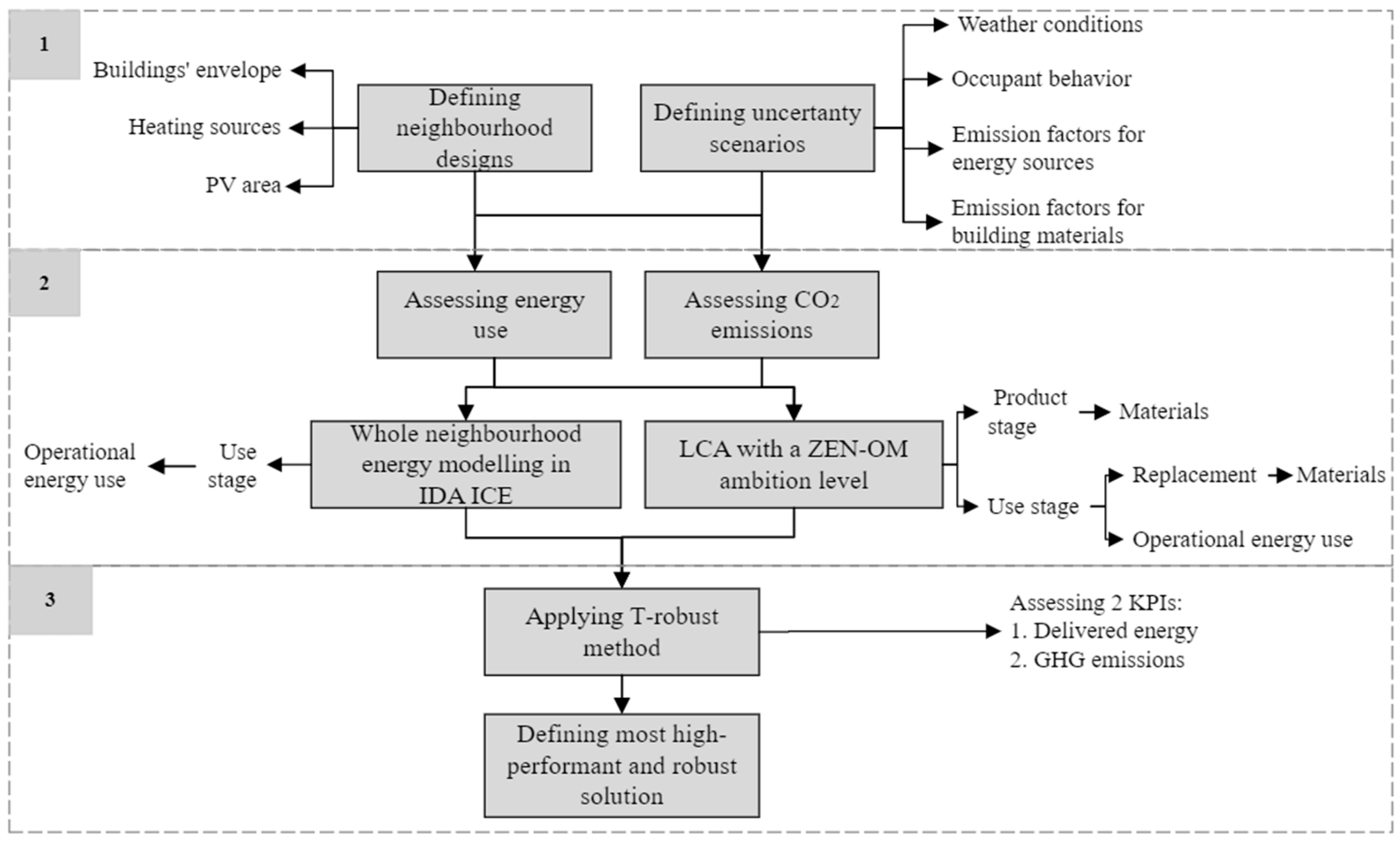
2.1. Overall Approach

The methodological approach outlined in this article is illustrated in Figure 1.
The first step involves defining neighborhood designs for further analysis. This includes selecting the main characteristics for the building’s envelope, heating sources, and available photovoltaic (PV) areas. Additionally, this step involves defining scenarios based on uncertainty factors such as weather conditions, occupant behavior, and emission factors for energy sources and building materials.
In the second step, the energy use of the whole neighborhood is assessed through detailed modeling for each design under each uncertainty scenario. Additionally, an LCA is conducted for all designs to assess GHG emissions, aiming for a specific ZEN ambition level. The latter involves assessing both embodied carbon in the building material (from raw material supply to manufacturing) and the use stage (materials’ replacement and energy use during operation).
In the third step, the T-robust method developed in [3] is applied to assess two KPIs and calculate the MT-KPI, which integrates performance targets across multiple criteria into the decision-making process, thus eliminating the need for criteria weighting. The MT-KPI is defined based on the number of KPIs considered; for instance, Homaei and Hamdy [3] utilized two KPIs, while Moschetti et al. [4] expanded it to three. The MT-KPI penalizes infeasible solutions by incorporating a robustness margin for each KPI. Each KPI has a corresponding performance target and robustness margin that creates different performance zones, as illustrated in Figure 2. The calculation of the MT-KPI depends on these performance zones and is defined in Table 1 for the two KPIs considered in this study, KPI1 and KPI2. Here, KPIi,rel represents the relative performance of each indicator, based on the robustness margins (KPIi,m), and is calculated as shown in Equation (1).
K P I 1 , r e l = K P I 1 K P I 1 , m × 100 K P I 2 , r e l = K P I 2 K P I 2 , m × 100
Following the MT-KPI calculations, the minimax regret method [20] was used to evaluate the difference between each design’s MT-KPI value in each scenario and the minimum performance across all designs for that scenario. This difference is termed performance regret, as defined by the minimax regret method. The maximum performance regret indicates the greatest deviation for each design, representing the largest gap between its worst and best performance. Consequently, the most robust design is identified as the one with the smallest maximum performance regret across all scenarios. Further details on the T-robust method are given in Table A3 and Table A4 in Appendix A.

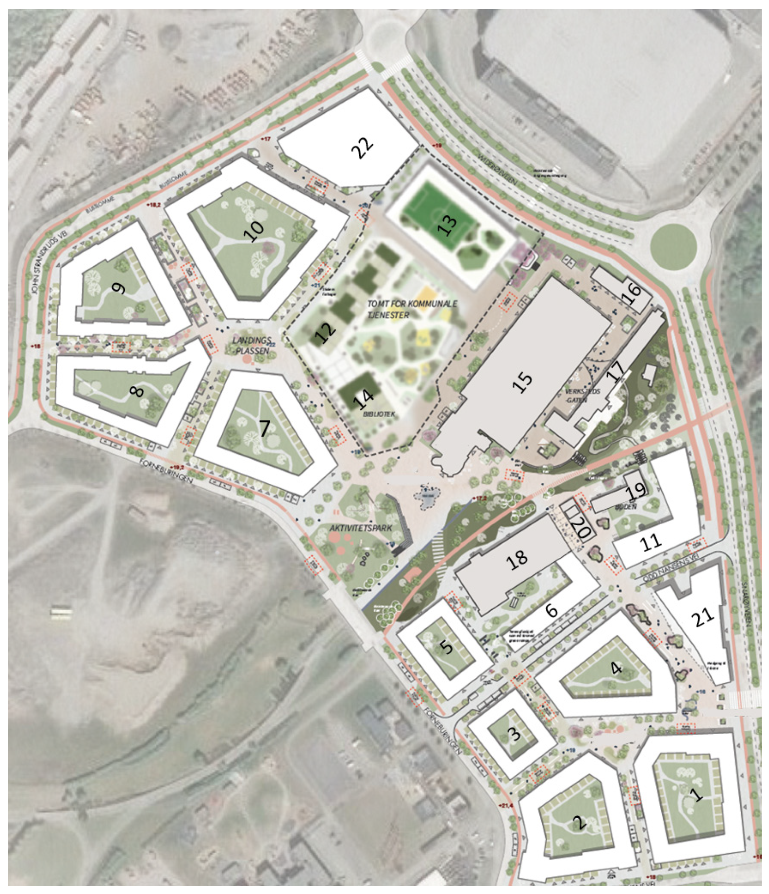
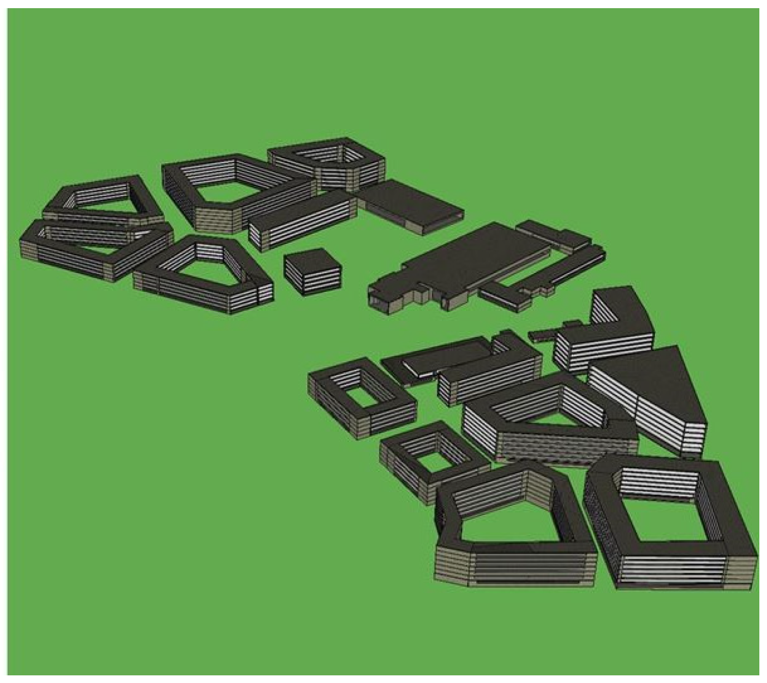
2.2. Case Study: Flytårnet Neighborhood

Flytårnet neighborhood is located within the Norwegian municipality of Bærum and aims to achieve zero-emission status by 2027. Consequently, evaluating climate and environmentally friendly solutions during the initial planning phase of Flytårnet was crucial. Figure 3 illustrates the neighborhood plan, while Table 2 provides the area of each building type.
The neighborhood currently comprises several existing buildings (indicated by gray areas in Figure 3), such as an air traffic control tower (area 15), repurposed as a cultural building, and a fire station (area 18), now functioning as an administration building. These existing buildings will undergo renovation and will be integrated into the new neighborhood, which will also include numerous newly constructed buildings serving various purposes, including apartment blocks, schools, sports facilities, and commercial establishments. Since the neighborhood was in the initial planning phase, detailed information about the construction type and materials for each building or building category was not yet available. Therefore, we analyzed different scenarios, as outlined in Section 2.4.

2.3. Analyzed Designs

In this study, four main designs were defined and analyzed based on input from the municipality that owns the case study neighborhood. Each design represents distinct combinations for both new and existing buildings, as follows: 1. standards that the building envelope must meet, 2. different heating sources, and 3. area allocated for photovoltaic (PV) installations.
Regarding the building envelope, Designs D1 and D3 comply with the Norwegian building technical regulation TEK17 [21] for both existing and new buildings, while Designs D2 and D4 have existing buildings adhering to TEK17 and new buildings meeting the stricter Norwegian Passive House (PH) standards [22,23].
The heating sources, covering room heating and domestic hot water (DHW), also differ. Designs D1 and D2 utilize electric heating (EH) for existing buildings and district heating (DH) for new ones. In Designs D3 and D4, existing buildings use electric heating, but new buildings employ air-source heat pumps (HP).
Finally, the PV installations vary in area coverage: Designs D1 and D2 feature PV systems across all roof areas, Design D3 is limited to new buildings, and Design D4 includes PV systems solely on apartment blocks.
Table 3 outlines all the aforementioned key parameters employed for the analyzed designs.

2.4. Analyzed Scenarios

Sixteen alternative scenarios were identified to assess the effect of different uncertainties, including changes in climate conditions, CO2 emission factors for materials and energy systems, and occupant behavior.
Table 4 provides an overview of the uncertainty parameters within the analyzed scenarios.
Two weather files were evaluated to depict both current and future climatic conditions. The current climatic conditions were defined using a standard typical meteorological year (TMY) weather file in EPW format for the location of Fornebu, an area of Bærum municipality (Norway). Future climatic conditions in 2050 were determined by modifying the current conditions’ weather file using the “CCworldWeatherGen tool” [24], based on the General Circulation Model (GCM) HadCM3 and the IPCC’s A2 emission representing a medium-high scenario. The resulting weather file accounts for the potential impacts of climate change and represents possible future weather conditions for the year 2050 in Fornebu.
Regarding CO2 emission factors for energy sources, two alternatives were defined to represent low and high emissions for both electricity and district heating as energy sources. The analysis utilizes two alternative emission factors for electricity, reflecting the Norwegian and European electricity mixes. These factors are based on the Norwegian standard NS 3720:2018 [25], which provides guidelines for evaluating the life-cycle emissions of buildings. The first CO2 emission factor for electricity reflects the Norwegian consumption mix based on the average from the past three years, projecting a transition to zero emissions by 2050 in line with national climate targets. The second CO2 emission factor for electricity employs the European consumption mix, also based on the average over the last three years, with a planned linear decline in emissions toward a near-zero production mix by 2050. For district heating, the first emission factor was chosen based on the mix of energy carriers currently used for district heating generation at the national level [26]. This consists of 52% waste heat, 21% bioenergy, 12% electricity, 12% ambient heat, and 3% fossil gas. The second emission factor for district heating was derived from the combination of energy carriers used by the district heating company supplying heat to the analyzed neighborhood [27]. This consists of 92% ambient heat, 4% bioenergy, and 4% electricity. The combination of low and high values for CO2 emission factors for energy sources is presented in Table 5.
In the assessment of CO2 emission factors for building materials, both typical and low-carbon materials were considered, with the latter having lower GHG emissions.
For new buildings, CO2 emission factors for various building categories with representative components and materials were sourced from existing literature focused on the Norwegian context [28,29]. This literature provides emissions data per square meter across several building categories, characterized by either typical or low-carbon materials. Since information on building components and materials for Flytårnet was unavailable, we referred to the data in [28,29], which also describe the building categories within the analyzed neighborhood. These categories are primarily defined by buildings with a concrete/steel load-bearing system, highly insulated external walls constructed with a wooden framework, concrete-based slabs, and roofs, as well as triple-glazed wooden windows with aluminum cladding. As a result, concrete constitutes approximately 80% of the total building mass. Replacing conventional concrete with low-carbon alternatives yields an average CO2 emissions reduction of 10%. Steel, used in columns and beams, represents 1–3% of the total mass of the model buildings yet accounts for 9–20% of the total emissions. Employing steel columns and beams with a higher proportion of scrap steel leads to an average emissions reduction of 6% across the model buildings. Additional measures identified in [28,29] for low-carbon alternatives include the use of untreated pine cladding, the replacement of ceramic tiles with vinyl, and the substitution of standard insulation with glass wool. It is worth noting that, according to the referenced sources, shifting to low-emission materials does not affect the thermal performance or energy efficiency of the buildings in the neighborhood.
For existing buildings, an energy upgrade was implemented to comply with the current minimum energy requirements established in TEK17. This upgrade included the addition of insulation to external walls, roofs, and ground floors, as well as the replacement of existing windows with more efficient triple-glazed alternatives. The greenhouse gas (GHG) emission values associated with the insulation and window products used in this upgrade were obtained from Norwegian Environmental Product Declarations (EPDs). Both low and high GHG emission values were considered to represent conventional and environmentally friendly alternatives, respectively [30,31,32,33,34,35]. Table A1 in Appendix A illustrates the CO2 emission factors used for both new and existing buildings within the Flytårnet neighborhood.
Similarly, for PV panels, EPDs of different technologies were considered to determine low and high values for both conventional and environmentally friendly alternatives [36,37].
Occupant behavior significantly affects building energy performance [38]. Our study examines two distinct occupant types: active and passive. Active users customize their behaviors based on outdoor conditions and implement energy-conscious measures. In contrast, passive users engage less and do not adopt energy-saving practices.
On the one hand, passive occupant behavior maintains a constant room set-point temperature according to NS 3031:2020 [39] across all building categories. This behavior assumes consistent occupancy for apartment blocks based on EN 16798-1 [40] and occupancy for other building categories according to NS 3031:2020. It also employs specific power usage based on NS 3031:2020 for electrical equipment features in different building categories, as well as a luminous efficacy of 12 lm/W for lighting.
On the other hand, active occupant behavior incorporates a 3 °C setback temperature at night for all building categories. It assumes occupancy for apartment blocks and offices, with two days of home office per week, while maintaining the same schedules as passive behavior for other building categories. Occupancy schedules for apartment blocks [41] were further differentiated by age groups (under 30 years, 30–64 years, and over 64 years) [42] for active behavior, whereas a uniform age group mix was applied for passive behavior. Active users employ electrical equipment with 10% higher efficiency than that specified in NS 3031:2020. Finally, lighting in active behavior uses LED lights with a luminous efficacy of 60 lm/W. Table A2 in Appendix A summarizes the main parameters for simulated occupant behaviors.

2.5. Analyzed Performance Indicators and Targets

Based on the preferences of the project owner (Bærum municipality), two main KPIs were assessed, and a target value and a robustness margin were defined for each KPI, as required by the T-robust method.
The first KPI focuses on delivered energy (for heating, DHW, mechanical ventilation, electric appliances, and lighting) during the use life cycle stage (B6). The target value for this KPI is based on the requirements of the Norwegian energy labeling system [43], which sets delivered energy values in different energy classes for different building categories. The delivered energy for the whole neighborhood in the best energy class was calculated. The calculated value was reduced by an assumption of 50% to achieve the zero-emission ambition of Flytårnet [44]. Note that in the calculation of the target for delivered energy, the contribution of the energy generated by PV is neglected. A 5% robustness margin was applied to the KPI based on the authors’ assumption and findings from previous studies [3].
The second KPI focuses on GHG emissions associated with the production stage (A1–A3) and two modules in the use stage: replacement (B4), as well as operational energy use, including on-site energy (B6). The target value is derived from the sum of target values in each of the life cycle stages considered. For GHG emissions related to building material production and replacement (A1–A3 and B4), the target value is calculated by multiplying the low identified emission factor for each building category as given in [28] by the respective building areas and then summing them up. Additionally, for PV panels, the target value is defined by multiplying the maximum available area for installing PVs on the roofs of the buildings in the neighborhood by the lowest emission factor among the two values considered in our calculations, specifically that related to environmentally friendly materials. For the GHG emissions associated with a building’s delivered energy (B6), the target value is defined by multiplying the first KPI target by the lowest emission factor for electricity as the most used source of energy in Norway. It was assumed that the robustness margin allows a 5% tolerance from the performance target. Table 6 illustrates the target values and correspondent robustness margins for each of the KPIs analyzed in this study.

2.6. Energy Modeling of Flytårnet Neighborhood

A comprehensive model of the neighborhood under study, encompassing all identified designs and scenarios, was developed (Figure 4) using the dynamic simulation software “Indoor Climate and Energy software” (IDA ICE) version 4.8. This software has undergone validation in numerous studies adhering to CEN standards and ASHRAE standards [45,46]. Modeling the neighborhood with IDA ICE enabled the analysis of energy consumption and generation on an hourly basis, which is important for understanding the real-time dynamics of energy use. This level of detail allows for precise evaluation of self-produced electricity consumption patterns within the neighborhood, as well as potential exports to the grid. Moreover, this model is flexible, allowing the consideration of various simulation factors, such as different climates and specific parameters related to occupant behavior.
Concerning the building envelope, various U-values for external building components, infiltration rates, and thermal bridge values were employed, based on the Norwegian building technical regulation TEK17 and PH standards. The primary parameters for envelope and building systems are provided in Table 7.
Heat gains and schedules related to internal loads, such as occupants, electric equipment, and artificial lighting, were set up for each building category according to the Norwegian standard NS 3031:2020 and the European standard EN 16798-1. Regarding the main technical systems of the buildings, heating set-points, ventilation air flows, and DHW, energy use was determined for each building category based on NS 3031:2020. This standard also served as the principal reference for the operational schedules of the technical systems. A balanced ventilation system was assumed for all designs in accordance with the Norwegian TEK17 standard. Additionally, the coefficient of performance (COP) for the heat pump was set as 3.5 for the designs, including the air-source heat pump.
The hourly energy generation from PV was determined through IDA ICE software based on the allocated PV area varying among the designs being considered for the neighborhood (see Table 3). The estimation of generated energy depended on factors such as varying yearly weather conditions and system efficiency (set to 18%), along with the available roof area. The orientation of the PV panels was set to face south, with an inclination of 30°, which was determined to be the most effective combination for energy generation.

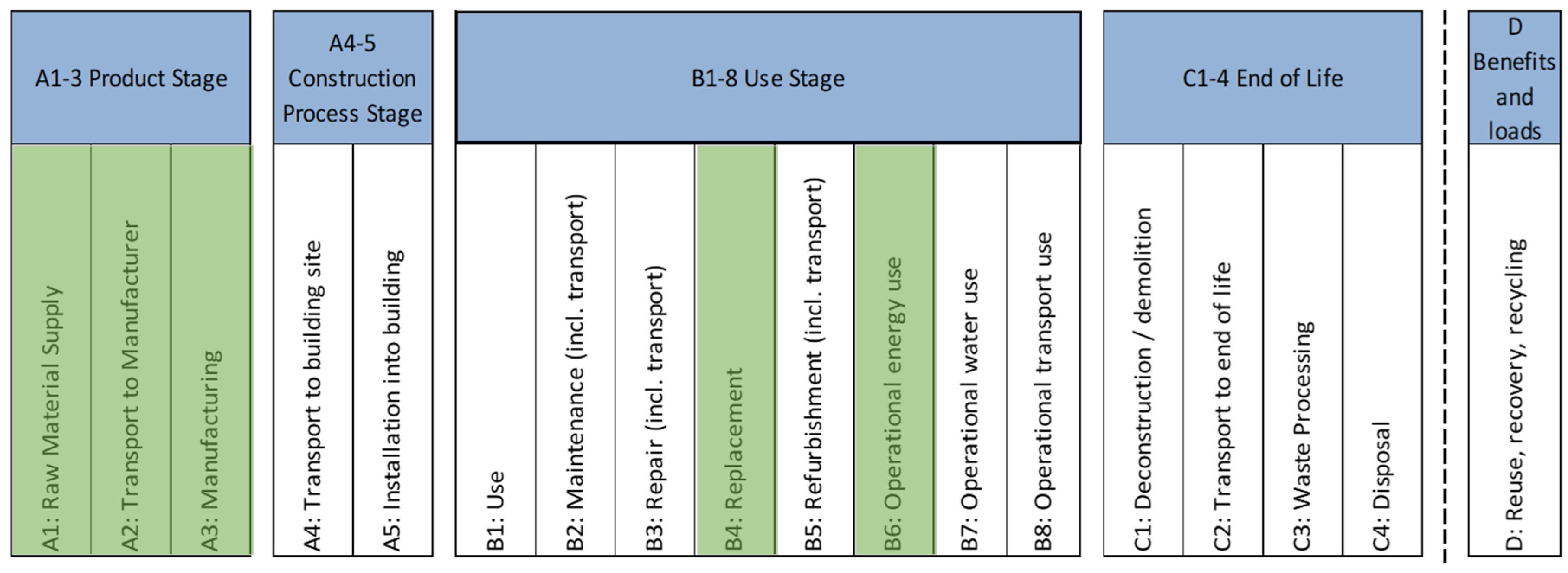
2.7. LCA of Flytårnet Neighborhood

A life cycle assessment (LCA) model was developed for Flytårnet, with the primary focus of quantifying GHG emissions associated with the following neighborhood components: buildings and on-site energy generation system (PV). Mobility, including transportation infrastructure as well as its emission and energy use, falls outside of the scope of this article.
This study adopted the “ZEN-OM” ambition level, covering the production stage (A1–A3), replacements (B4), and operational energy use (B6) throughout the life cycle of the neighborhood. The stages mentioned are illustrated in Figure 5. ZEN-OM is among the ambition levels proposed by Laulesset et al. [47] for achieving carbon neutrality in a zero-emission neighborhood. These levels stem from the recommendations outlined by the FME ZEB known as the “Zero-emission Buildings (ZEB) definition” [48]. The framework involves integrating various life cycle modules, spanning from A1 to C4. The selection of specific modules depends on the ambition level set by the project owner.
The ambition levels, adapted from the ZEB definition, are described as follows:
  • ZEN O: Addresses emissions solely related to operational energy (“O”), specifically module B6.
  • ZEN OM: Encompasses both operational energy (“O”) emissions and embodied emissions from materials (“M”) and their replacement, covering modules A1–A3 and B4, B6.
  • ZEN COM: Similar to ZEN OM, this level includes also emissions from the construction (“C”) stage, incorporating modules A4–A5.
  • ZEN COME: Expands upon ZEN COM by also considering emissions from the end-of-life (“E”) stage, covering modules C1 to C4.
The analysis period in our analysis spans 60 years, corresponding to the assumed lifetime of buildings.

2.7.1. Product and Replacement Stages (A1–A3, B4)

The GHG emissions of the neighborhood in the production and replacement stages were defined by summing up the GHG emissions from the construction of all new buildings and their renovation during the neighborhood lifespan, together with the GHG emissions from the materials used for upgrading the existing buildings and the standard material replacement in these buildings. This top-down approach for the LCA model was adopted because, with the neighborhood in an early planning stage, detailed information on the construction type and materials for each building or building category was not available. GHG emissions for new and existing buildings were defined by multiplying emission factors, as shown in Table A1, by the area of each building category and then summing them up. For both new and existing buildings, both the product stage (A1–A3) and the material replacement stage (B4) were considered.
Equation (2) shows the calculation of the total embodied emissions in neighborhood buildings, Ebuild (kg CO2 eq.), for the product and replacement stages, over a 60-year period.
E b u i l d = b c ,   n e w E m a t , i n i t b c , n e w × A b c , n e w + i = 0 60 E m a t , r e p l . i , b c , n e w × A b c , n e w + b c ,   e x E m a t , i n i t b c , e x × A b c , e x + i = 0 60 E m a t , r e p l . i , b c , e x × A b c , e x
where Emat,init,bc,new stands for the emissions embodied in the materials initially contained in the new buildings, expressed per building floor area and year (kg CO2-eq./m2/yr); Abc,new is the area of the new building categories (m2); Emat,repl,bc,new represents the emissions embodied in the materials used in replacements for new buildings, expressed per building floor area and year (kg CO2-eq./m2/yr); i is the year over a 60-year period; Abc,ex is the area of the existing building categories (m2); Emat,init,bc,ex stands for emissions embodied in the initial materials for upgrading specific components in existing buildings, expressed per building floor area and year (kg CO2-eq./m2/yr); and Emat,repl,bc,ex represents the emissions embodied in the materials used in replacements for existing buildings, expressed per building floor area and year (kg CO2-eq./m2/yr).
Further details regarding the GHG emission assessment are provided in Section 2.4.

2.7.2. Operational Energy Use (B6)

The operational energy use involves in this study the delivered energy, which was calculated using the IDA ICE model developed for the neighborhood, accounting for different designs and uncertainty scenarios. It is assumed that the delivered energy over the 60-year calculation period is the sum of the equal contribution from each year, with loads (such as weather and internal gains) remaining constant throughout the analysis period. More details about the energy systems across different designs and the emission factors for various energy sources are provided in Section 2.4.
The locally generated electricity is expected to lead to negative (i.e., avoided) emissions, as the PV panels offset a portion of the electricity demand of the buildings, thereby reducing dependence on external grid electricity.
Equation (3) illustrates how the neighborhood buildings’ energy need calculated by IDA ICE is employed to define the energy delivered to buildings, DEbuild (kWh), over a 60-year period.
D E b u i l d = b u i l d i = 0 60 h = 0 8640 D E e l ( E l n e e d , i , h E l P V , i , h ) × E l e f f + i = 0 60 h = 0 8640 D E t h e r m E n n e e d , t h e r m , i , h × D H e f f × Y t h e r m
where ∑build stands for summation over contributes from new and existing buildings; i represents the year over a 60-year period; h is the hour over a year; DEel is the electricity delivered to buildings; Elneed stands for the electricity demand (kWh); ElPV is the electricity generated by PV (kWh); Eleff represents the efficiency of the electric system, either as direct electricity or electric heat pump (kWh); DEtherm is the thermal energy delivered to buildings via district heating; Enneed,therm is the thermal energy demand; DHeff is the efficiency of district heating; and Ytherm is a binary variable, with Ytherm = 1 if the building’s thermal energy is provided by district heating network or Ytherm = 0 if electricity is the only energy source for the building.
Equation (4) shows the calculation of GHG emissions from energy delivered to all buildings, EDE,build (kg CO2 eq.), over a 60-year period.
E D E , b u i l d = b u i l d D E e l × E e l + D E t h e r m × E D H × Y t h e r m
where ∑build stands for summation over contributes from new and existing buildings; DEel electricity delivered to buildings; Eel is the emission factor for electricity (kg CO2 eq./kWh); DEDH energy delivered to buildings via district heating; and EDH is the emission factor for district heating (kg CO2 eq./kWh).
Equation (5) shows the calculation of GHG emissions from a neighborhood’s on-site energy generation system, i.e., the PV system, EPV (kg CO2 eq.), over a 60-year period.
E P V = r o o f , P V   E P V , i n i t ×   A P V r o o f , P V + i = 0 60 E P V , r e p l × A P V i , r o o f , P V
where ∑roof,PV is the summation over contributions from all building roofs with PV panels; EPV,init is the factor for embodied emissions in initial PV panels (kg CO2 eq./m2); EPV,repl is the factor for embodied emissions in PV panels used in replacement (kg CO2 eq./m2); i represents the year over a 60-year period; and APV is the area of PV panels (m2).
It is worth noting that EPV,init and EPV,repl were set to be equal in our analysis.
The GHG emissions for the whole neighborhood, Eneigh,tot (kg CO2 eq.), over a 60-year period, are calculated as shown in Equation (6).
E n e i g h , t o t = E b u i l d + E D E , b u i l d + E P V
where Ebuild represents the total GHG emissions embodied in neighborhood buildings for the production and replacement stages (A1–A3 and B4); EDE,build stands for GHG emissions from energy delivered to all neighborhood buildings (B6); and EPV represents the GHG emissions from the PV system throughout the neighborhood (B6).

3. Results

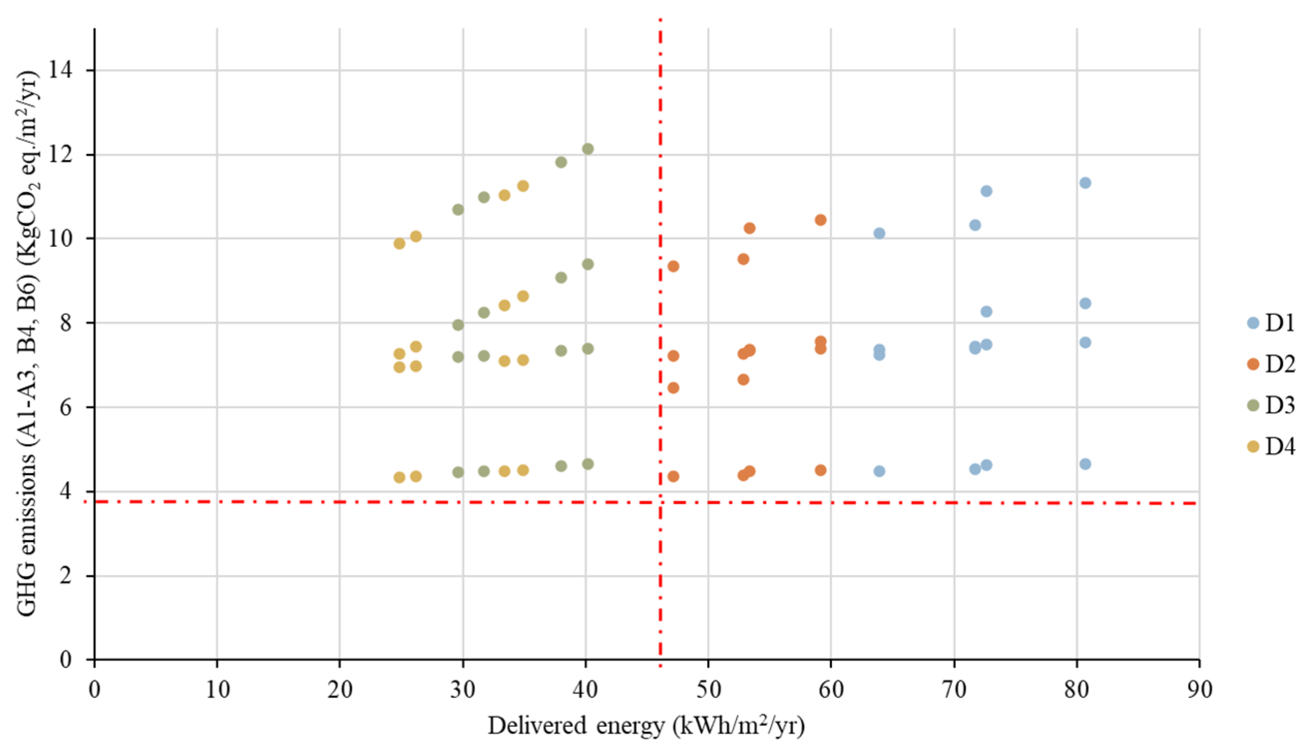
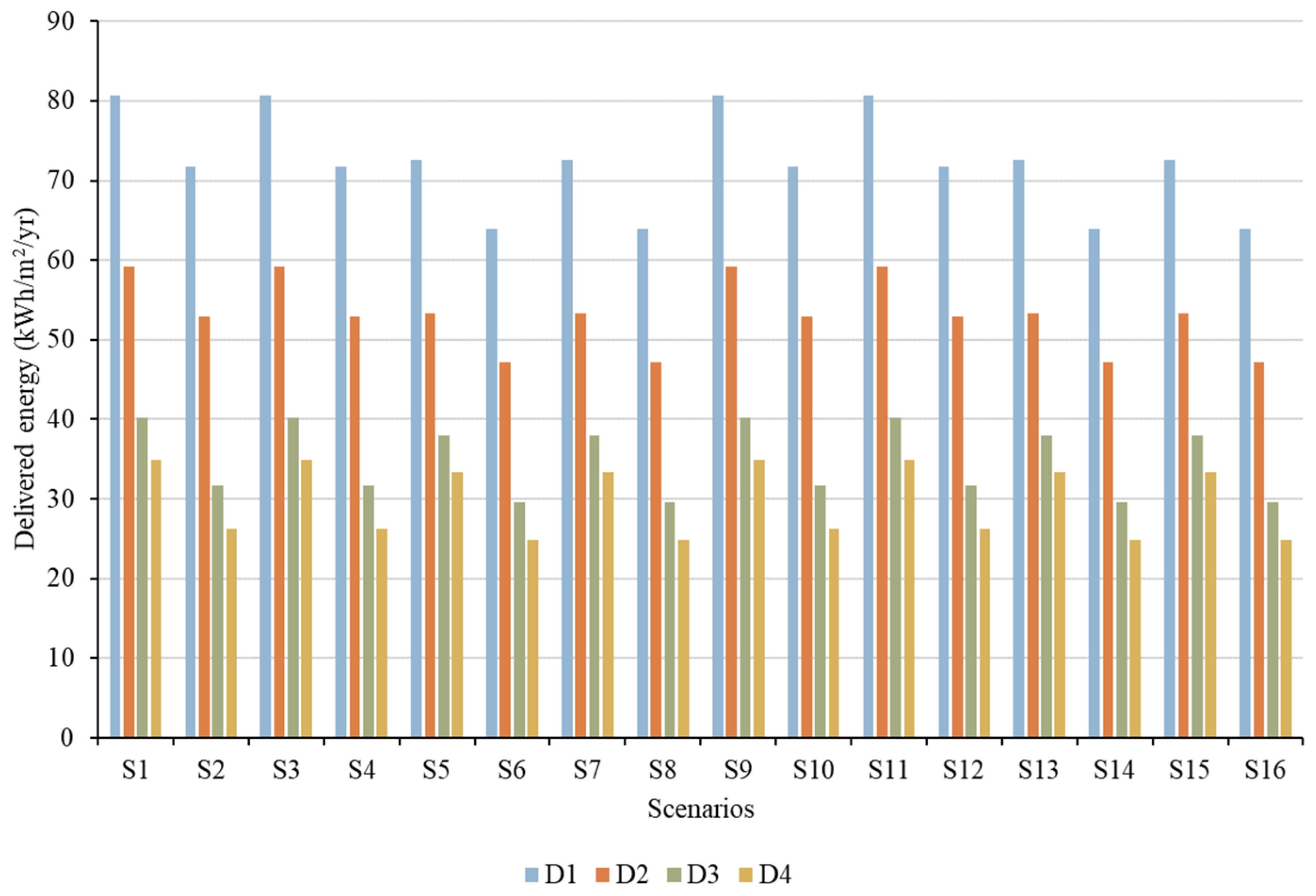
3.1. Performance Assessment of Designs and Scenarios Using KPIs

Figure 6 illustrates the results for the first KPI for the four designs across sixteen uncertainty scenarios, expressed per total neighborhood building floor area and year, over a 60-year period. D1 consistently has the highest delivered energy among the four designs, reaching up to approximately 80 kWh/m2/yr, due to its compliance with the less stringent building standard (TEK17) and the use of district heating as the heating source. In contrast, D4 has the lowest delivered energy, achieving as low as approximately 25 kWh/m2/yr, attributed to the implementation of the more stringent PH standard and the use of heat pumps in the new buildings. When it comes to the scenario options, using the 2050 weather file in the neighborhood simulation results in lower delivered energy compared with the current weather file. This is primarily because cooling energy demand is not considered in our calculations, and heating energy demand decreases with higher temperatures in 2050. Additionally, active occupant behavior reduces delivered energy levels. The scenarios combining the 2050 weather file with active occupant behavior—specifically S6, S8, S14, and S16—yield the lowest delivered energy for all designs.
Figure 7 illustrates the results for the second KPI for the four designs across sixteen uncertainty scenarios, ex-pressed per total neighborhood building floor area and year, over a 60-year period. The results, ranging from approximately 4 to 12 kg CO2 eq./m2/yr, indicate that the most influential factor is the selection of high versus low emission factors for energy sources and materials. There is a marked difference between the low-emission scenarios (S1, S2, S5, S6, S9, S10, S13, S14) and the high-emission scenarios (S3, S4, S7, S8, S11, S12, S15, S16). Since material emissions have been included as a scenario option, the amount of material emission is the same in different designs, and the evaluated emissions primarily reflect the use stage emissions. This is particularly evident in high-emission scenarios due to the greater difference in emission factors for electricity and district heating. In these high-emission scenarios, D2 has the lowest emissions due to the use of district heating and passive house standards for the new building. Conversely, D3 shows the highest emission because of the use of electricity as the heat source and TEK17 as the building standard in new buildings. For the low-emission scenarios, all designs exhibit emissions within a similar range. However, there is competition between D2 and D4 for having the lowest emission in low-emission scenarios. This highlights the complexity of comparing GHG emissions at an aggregate level across designs under different uncertainties.
Figure 8 shows the distribution of GHG emissions across the four designs within two exemplary scenarios. The figure demonstrates how different scenarios influence GHG emissions, depending on factors like weather files, emission factors, and occupancy behavior. This finding highlights the importance of evaluating uncertainties in the neighborhood design, as well as selecting a robust design. These results are in line with those of similar studies [14,15].
Figure 9 shows the results of all designs across all scenarios considering the two KPIs. The red lines show the robustness margin values of each KPI. As can be seen, none of the designs meet the performance target regarding both KPIs. By analyzing Figure 9, the following points can be observed:
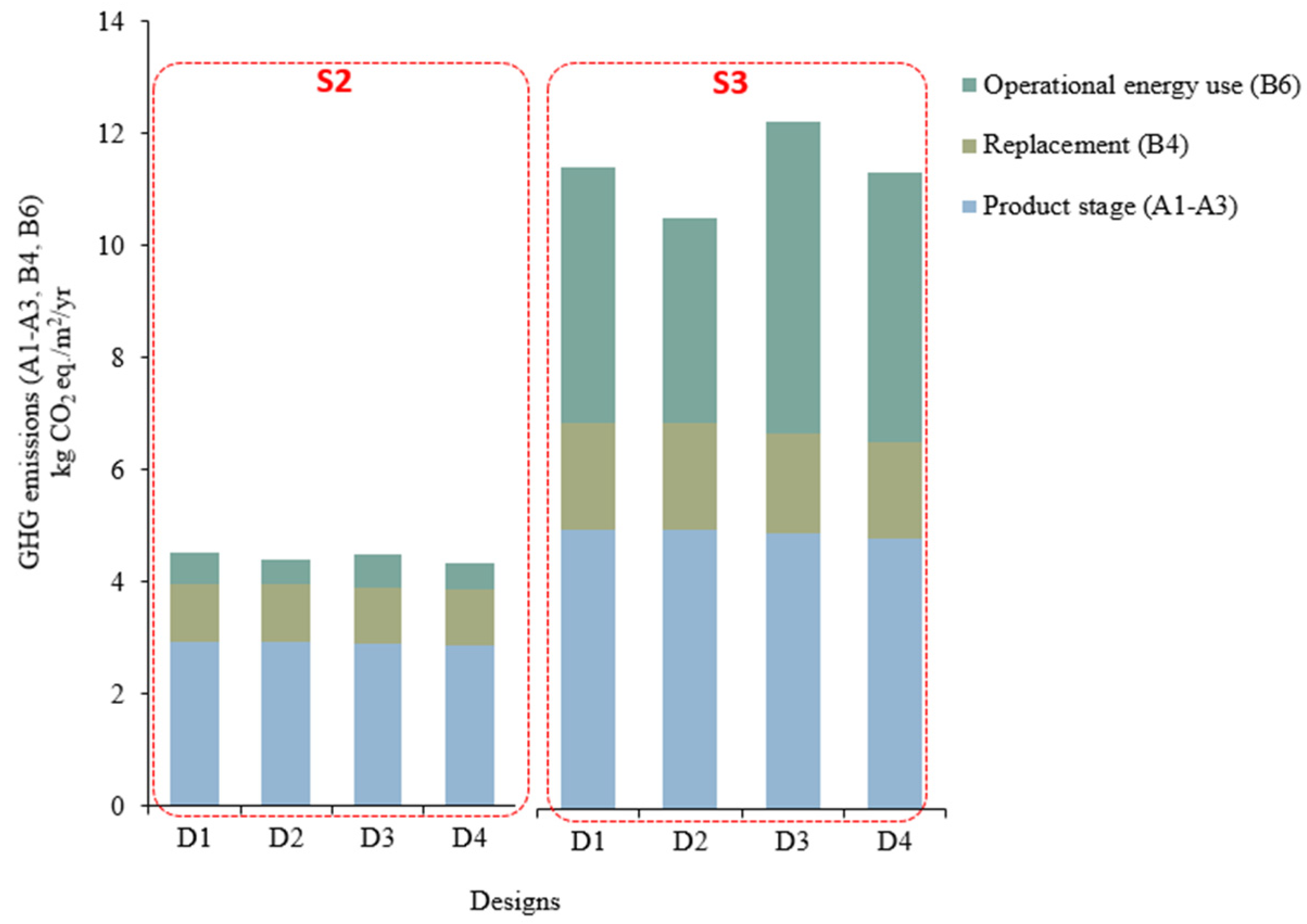
  • Regarding the robustness margin of GHG emissions, all designs will experience GHG emission values higher than 3.9 kg CO2/m2/yr under all scenarios. It can be observed from Figure 9 that in low-emission scenarios, all designs perform within a similar range, but in high-emission scenarios, the performance of designs is more distributed.
  • When it comes to KPI 1, about operational energy use, D3 and D4 meet the robustness margin in all scenarios, while D1 and D2 consistently perform worse than the robustness margin. This indicates that D1 and D2 are less robust in terms of KPI 1.
Figure 9. GHG emissions (A1–A3, B4, B6) vs. delivered energy for the four designs across uncertainty scenarios (the red lines show the robustness margins).
Energies 17 06210 g009
However, comparing even just the two designs (D3 and D4) that appear to perform best with respect to two KPIs is neither straightforward nor resource-efficient in real-world scenarios, as observed in our study. The choice of the best design among those analyzed is complex and becomes even more challenging with a greater number of designs and scenarios. Therefore, the T-robust method was used to assist decision-makers in selecting the most robust and high-performance design.

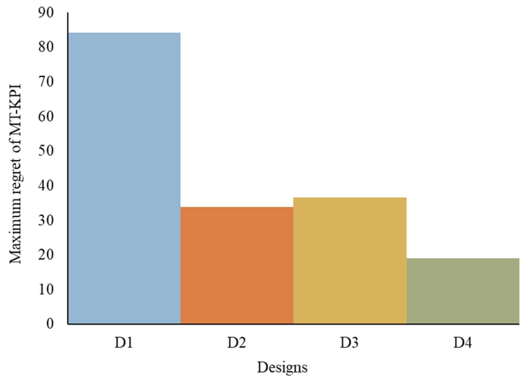
3.2. Robustness-Based MCDM Assessment

Figure 10 presents the results of the robustness assessment using the MT-KPI. As shown in the figure, D4 emerges as the most robust and high-performance neighborhood design based on the maximum regret indicator, having the lowest maximum regret value among all designs.
The MT-KPI calculations for each design under every scenario were executed using an automated MATLAB [50] algorithm. Similarly, the minimax regret method calculations were also automated using MATLAB, with the corresponding formulas detailed in Appendix A (Table A3 and Table A4).
A key advantage of the T-robust method is its automatic establishment of preferences using performance targets. Considering the specified performance targets for GHG emissions and operational energy use, D4 deviates less from these targets and proves to be the most robust design in the face of future uncertainties.

3.3. Test Conditions for KPI 2

To assess the impact of the selected life cycle modules on the analysis, the T-robust method was applied under two different test conditions (T). Each test condition involves different life cycle stages in the calculation of KPI 2, as shown in Table 8. It is important to note that KPI 1 remains consistent for both T1 and T2. In T1, KPI 2 includes only operational energy use (B6), aligning with the ZEN-O ambition level, as outlined in Section 2.7. Conversely, in T2, KPI 2 incorporates only building material and replacement (A1–A3, B4) emissions. As can be seen in Table 7, the selected robust design is different in T1 and T2. When KPI 2 focuses solely on operational energy use emissions, D2 is identified as the most robust design. Even though D3 and D4 perform similarly well in terms of operational energy use, D2 deviates less from the emission target across all scenarios and is therefore chosen as the most robust design by the T-robust method. On the contrary, when KPI 2 focuses only on building material and replacement emissions, D4 is selected as the most robust design. This is because, in T2, KPI 1 is the same as in T1 for all designs, and D4 performs better under uncertainties related to KPI 2 (see Figure 11), leading the T-robust method to select it as the most robust design. This finding is also in line with the selected design when emissions include both material and use phase emissions (Section 3.1). The analysis shows how excluding certain elements in emission calculations and neglecting uncertainties can lead decision-makers to select an inappropriate design and highlights the importance of considering a comprehensive range of GHG emissions from different sources in selecting a robust design.

4. Discussion

The results on GHG emissions and operational energy use align with findings from similar studies [18]. However, direct comparison is challenging due to variations among neighborhoods in terms of included building typologies and discrepancies across studies stemming from differences in incorporated built environment components and analyzed life cycle stages.
The first research question identified in this article, concerning how to comprehensively understand energy use and GHG emissions across various life cycle stages to inform neighborhood performance assessment and design decisions, is addressed through a holistic approach. This involves evaluating the energy and environmental impact at different stages of a neighborhood’s development, from initial planning and construction to operation. The use of integrated modeling tools, with parallel energy and LCA modeling, is also essential to assess trade-offs between design alternatives and uncertainty scenarios.
The second research question, exploring the advantages and challenges of integrating robustness assessment and MCDM for neighborhood performance evaluation, highlights several key considerations. The primary advantage is the ability to assess performance against multiple criteria and under various future scenarios and uncertainties. This enhances the robustness of design decisions and helps stakeholders prioritize different criteria according to project goals and community needs. It also facilitates the identification of optimal solutions that balance competing objectives, such as minimizing emissions while maximizing energy efficiency.
However, challenges arise from the complexity of modeling and the need for extensive data collection, which can be resource-intensive. The accuracy of data is critical to ensure valid assessments and reliable decision-making. Addressing uncertainties, such as future climate conditions and occupant behaviors, requires careful scenario planning. Ensuring that assessments capture these uncertainties and provide reliable guidance for decision-makers is difficult. Therefore, creating user-friendly tools for analysis, based, e.g., on the algorithms used in this study, will facilitate understanding and accessibility, enabling stakeholders to engage more effectively in the decision-making process.
Balancing multiple, often conflicting criteria is also challenging, particularly when stakeholders have varying priorities. Therefore, developing standardized guidelines that address the relative importance of different criteria and acceptable trade-offs is crucial for the successful implementation of this approach.
When assessing this article’s results, several critical parameters emerged, as follows:
  • The building envelope significantly influences the comparison of different neighborhood designs and the choice of the most robust design. The chosen energy standard, whether it is stringent like PH or less strict like TEK17, leads to varying energy demand, impacting both energy consumption and GHG emissions during the neighborhood’s life cycle.
  • The selection of high- or low-emission materials affects emissions related to material production and replacement stages, which can have a greater impact than energy-use-related emissions, particularly in low-carbon grid contexts like in Norway. In such settings, achieving full compensation for the life cycle GHG emissions from materials remains challenging, even with extensive use of PV panels. D2 is, for instance, the design with the highest allocated area for PVs among those assessed, and this contributes to its selection as the most robust design when only the neighborhood’s use stage is considered. However, when other life cycle stages are also considered, D2 loses its position as the most robust design.
  • Emission factors for energy sources also have a critical role in determining the final design choice. When focusing solely on the operational energy stage, some designs may show low delivered energy but emit high levels of GHG during the use stage. The discrepancy in CO2 emission factors between district heating and electricity stems from the energy carriers used in heat production. Norwegian standards, such as the Norwegian NS 3720, often consider recovered heat in district heating as environmentally friendly since it avoids the consumption of primary energy sources. As a result, emissions from district heating are allocated solely to the original activity generating the waste heat rather than to the district heating process itself. In contrast, electricity production typically involves higher emission factors, although still lower than the average European level. Thus, careful consideration of these emission factors is crucial when designing environmentally sustainable systems, particularly when choosing specific energy sources.
  • The selection of life cycle modules for GHG emission calculation is crucial in determining the most robust design using the T-robust method. This approach helps decision-makers choose GHG emission indicators more effectively under future uncertainties. In this study, when the indicator focuses solely on operational energy emissions, D2 proves to be the most robust design due to its use of a low-emission energy source and the largest allocated PV area. However, when GHG emissions also account for materials, replacement, and operational energy, D4 emerges as the most robust option due to its lower overall energy consumption and reduced deviation from the emission target. Although D4 has higher operational phase emissions, its overall performance in terms of both material and energy emissions is superior. This demonstrates how the choice of life cycle elements in indicator assessments can significantly influence decision-making, potentially leading to suboptimal design choices. The T-robust method effectively captures these nuances, aiding decision-makers in selecting robust designs without the complexity of comparing multiple indicators. Incorporating LCA from the early planning stages ensures more informed decision-making by accounting for both embodied and operational emissions, leading to a more comprehensive assessment of a building’s environmental impact.
Certain limitations of this study should be considered to facilitate the comparability of the results. Firstly, the LCA model does not account for long-term technological advancements and improvements in production processes, which can lead to emission reduction over time in a 60-year analysis period. Further research is needed to predict more accurate scenarios for material production improvements. The LCA model also faces uncertainties regarding emission intensities from buildings and energy sources, which are specifically tailored to the Norwegian context. Secondly, the energy model is based on assumptions that might affect result interpretation. For instance, two different occupancy patterns were assessed based on regulatory framework and possible improvements, but future patterns are often difficult to predict accurately. Furthermore, buildings’ thermal dynamics, including U-values and infiltration rates, might change over time and affect the overall neighborhood’s energy efficiency.

5. Conclusions

This article presents a comprehensive evaluation of neighborhood performance through a robustness-based multi-criteria approach, focusing on greenhouse gas (GHG) emissions and energy use across various life cycle stages. Using Flytårnet—a Norwegian neighborhood aiming for zero emissions by 2027—as a case study, the research explores the influence of building materials and energy sources on GHG emissions and energy use. By employing a case study methodology, the article aims to deepen our understanding of neighborhood performance dynamics.
The analysis incorporates the T-robust method, a robustness-based multi-criteria decision-making (MCDM) framework, to identify high-performance, resilient designs capable of withstanding uncertainties. Results indicate that buildings in the neighborhood receive 25 to 80 kWh/m2/year of energy during operation, including from photovoltaics. Over 60 years, life cycle GHG emissions vary from 4 to 12 kg CO2-eq./m2/year, accounting for uncertainties and covering material production, replacement, energy consumption, and generation. This study reveals that the optimal design varies significantly depending on whether the assessment focuses solely on the use phase or considers the full life cycle.
These findings highlight how different life cycle stages impact the selection of robust neighborhood designs. The research underscores the need for urban planners to integrate life cycle assessments (LCAs) early in the planning process, extending beyond operational performance to include embodied emissions from building materials. The T-robust method proves essential in accounting for uncertainties and ensuring long-term design resilience. For Flytårnet, this study demonstrates that designs optimized for operational energy may not perform as well when full life cycle emissions are included, emphasizing the importance of a holistic evaluation framework.
The article provides valuable guidance for decision-makers and designers striving to select high-performance, resilient neighborhood designs while navigating multiple conflicting performance criteria. It advances knowledge in sustainable neighborhood development and supports strategic urban planning. Additionally, this study addresses a gap in integrating comprehensive LCAs into neighborhood decision-making, especially for pre-use stages and embodied emissions from materials. Employing robustness-based multi-criteria analysis from the outset is crucial for zero-emission neighborhoods, as evaluating multiple designs under uncertainty through competing key performance indicators ensures robust solutions. The implemented robustness-based multi-criteria methodology in this paper, known as the T-robust method, is generic and can be used across different contexts, including different geographical environments and climatic conditions. Furthermore, the T-robust method can address multiple uncertainties, such as evolving market dynamics, regulatory changes, and technological advancements.
Future research could expand on the findings of this study by integrating additional factors, such as mobility, into neighborhood GHG and energy analyses and incorporating more life cycle stages, including end-of-life considerations. Further work could also focus on refining the research framework to accommodate different types and scales of communities, as well as validating its effectiveness across diverse case studies. Additionally, future studies could examine how specific characteristics influence outcomes, providing policymakers with more targeted and actionable recommendations. Finally, future research could also incorporate long-term monitoring mechanisms, enabling real-time validation and iterative refinement of the evaluation model based on observed performance data.

Author Contributions

Conceptualization, R.M. and S.H.; methodology, R.M. and S.H.; software, S.H.; validation, R.M. and S.H.; formal analysis, R.M. and S.H.; investigation, R.M. and S.H.; resources, R.M. and S.H.; data curation, R.M. and S.H.; writing—original draft preparation, R.M. and S.H.; writing—review and editing, R.M. and S.H.; visualization, R.M. and S.H.; supervision, R.M.; project administration, R.M.; funding acquisition, R.M. All authors have read and agreed to the published version of the manuscript.

Funding

This article has been written within the Research Centre on Zero Emission Neighbourhoods in Smart Cities (FME ZEN). The authors gratefully acknowledge the support from the ZEN partners and the Research Council of Norway (project no. 257660).

Data Availability Statement

Dataset available on request from the authors.

Conflicts of Interest

The authors declare no conflicts of interest.

Appendix A

Table A1. CO2 emission factors for all building categories, considering both typical and low-carbon materials.
CO2 Emissions Related to Life Cycle Stages
A1–A3, B4 (kg CO2 eq./m2/yr)
Type of BuildingTypical MaterialsLow-Carbon Materials
A1–A3B4A1–A3B4
Office buildings4.41.72.61.0
Apartment blocks5.41.63.21.0
Schools4.41.33.00.9
Commercial building3.81.52.41.0
Cultural buildings4.41.33.00.9
Sport buildings4.41.33.00.9
Existing buildings0.5 *1.2 **0.3 *0.9 **
* This average value includes additional insulation and new triple-pane windows for the upgrade of existing buildings. ** This average value accounts for materials replacements in standard maintenance for existing buildings as for new buildings.
Table A2. Parameters used in IDA ICE for simulating active and passive occupant behaviors.
Occupant Behavior
ActivePassive
Heating system_setpoint and scheduleTwo different temperatures
based on occupancy.
For apartments: 22 °C during day and 19 °C during night.
For sport buildings: 19 °C when occupied and 16 °C when not occupied.
For all other buildings: 21 °C when occupied and 18 °C when not occupied.
Constant temperature during day, i.e.,
22 °C for apartments,
19 °C for sport building,
21 °C for other building categories.
Building occupancy schedulesSame as occupancy for ‘’passive behavior’’ but considering 2 days home office per week.Occupancy for apartment blocks based on prEN16798-1 (employed).
Occupancy for other building categories based on NS 3031:2020.
Additional building occupancy schedule_only apartment blocksDifferent occupancy schedules based on age groups.
Non-uniform age group mix:
35% under 30 years
47% 30–64 year
17% over 64.
Same occupancy schedules for all apartment blocks (based on prEN16798-1) with uniform age group mix.
Electric equipment efficiency10% higher efficiency than in the “passive behavior”.Different for building categories, based on NS 3031:2020
Lighting efficiencyLED lights with luminous efficacy of 60 lm/W.Standard lights with luminous efficacy of 12 lm/W.
Table A3. Finding the maximum and minimum performance of a design across scenarios and best performance for designs and scenarios, from [4].
DesignScenariosMax and Min Performance Across Scenarios
S1S2SiSnMaximum
Performance (A)
Minimum
Performance (B)
D1KPI11KPI21KPIi1KPIn1A1 = max
(KPI11,…, KPIn1)
B1 = min
(KPI11,…, KPIn1)
D2KPI12KPI22KPIi2KPIn2A2B2
DiKPI1iKPI2iKPIiiKPIniAiBi
DmKPI1mKPI2mKPIimKPInmAmBm
Minimum performance for each scenario (C)C1 = min (KPI11,…, KPI1m)C2CiCn
Best performance of all designs across all scenariosD = min(B) = min(C)
Table A4. Robustness calculation using max–min, best-case and worst-case, and min–max regret methods, from [4].
Performance Regret (R)
DesignsScenarios
S1S2Sn
D1R11 = KPI11 − C1R21 = KPI21 − C2Rn1 = KPIn1 − Cn
D2R12 = KPI12 − C1R22 = KPI22 − C2Rn2 = KPIn2 − Cn
DiR1i = KPI1i − C1R2i= KPI2i − C2Rni = KPIni − Cn
DmR1m = KPI1m − C1R2m = KPI2m − C2Rnm = KPInm − Cn

References

  1. Salter, J.; Lu, Y.; Kim, J.C.; Kellett, R.; Girling, C.; Inomata, F.; Krahn, A. Iterative ‘What-If’ Neighborhood Simulation: Energy and Emissions Impacts. Build. Cities 2020, 1, 293–307. [Google Scholar] [CrossRef]
  2. Charani Shandiz, S.; Rismanchi, B.; Foliente, G. Energy Master Planning for Net-Zero Emission Communities: State of the Art and Research Challenges. Renew. Sustain. Energy Rev. 2021, 137, 110600. [Google Scholar] [CrossRef]
  3. Homaei, S.; Hamdy, M. A Robustness-Based Decision Making Approach for Multi-Target High Performance Buildings under Uncertain Scenarios. Appl. Energy 2020, 267, 114868. [Google Scholar] [CrossRef]
  4. Moschetti, R.; Homaei, S.; Taveres-Cachat, E.; Grynning, S. Assessing Responsive Building Envelope Designs through Robustness-Based Multi-Criteria Decision Making in Zero-Emission Buildings. Energies 2022, 15, 1314. [Google Scholar] [CrossRef]
  5. Homaei, S.; Moschetti, R.; Clauss, J. Selection of the Most High-Performance and Robust Design for a Zero-Emission Neighbourhood: Case Study of Flytårnet Area in Norway. In Proceedings of the Building Simulation 2023: 18th Conference of IBPSA, Shanghai, China, 4–6 September 2023; pp. 2415–2422. [Google Scholar] [CrossRef]
  6. Weiler, V.; Eicker, U. Automatic Energy Demand and System Simulation at District Level. Nachhalt. Manag. Forum 2021, 29, 133–141. [Google Scholar] [CrossRef]
  7. Li, W.; Zhou, Y.; Cetin, K.; Eom, J.; Wang, Y.; Chen, G.; Zhang, X. Modeling Urban Building Energy Use: A Review of Modeling Approaches and Procedures. Energy 2017, 141, 2445–2457. [Google Scholar] [CrossRef]
  8. Swan, L.G.; Ugursal, V.I. Modeling of End-Use Energy Consumption in the Residential Sector: A Review of Modeling Techniques. Renew. Sustain. Energy Rev. 2009, 13, 1819–1835. [Google Scholar] [CrossRef]
  9. Kavgic, M.; Mavrogianni, A.; Mumovic, D.; Summerfield, A.; Stevanovic, Z.; Djurovic-Petrovic, M. A Review of Bottom-up Building Stock Models for Energy Consumption in the Residential Sector. Build. Environ. 2010, 45, 1683–1697. [Google Scholar] [CrossRef]
  10. Nageler, P.; Koch, A.; Mauthner, F.; Leusbrock, I.; Mach, T.; Hochenauer, C.; Heimrath, R. Comparison of Dynamic Urban Building Energy Models (UBEM): Sigmoid Energy Signature and Physical Modelling Approach. Energy Build. 2018, 179, 333–343. [Google Scholar] [CrossRef]
  11. Kong, D.; Cheshmehzangi, A.; Zhang, Z.; Ardakani, S.P.; Gu, T. Urban Building Energy Modeling (UBEM): A Systematic Review of Challenges and Opportunities. Energy Effic. 2023, 16, 69. [Google Scholar] [CrossRef]
  12. Lausselet, C. The Use of LCA Methods for Evaluating and Planning Netzero-Emission Neighbourhoods. Ph.D. Thesis, NTNU, Trondheim, Norway, 2021. [Google Scholar]
  13. Hachem, C. Impact of Neighborhood Design on Energy Performance and GHG Emissions. Appl. Energy 2016, 177, 422–434. [Google Scholar] [CrossRef]
  14. Moschetti, R.; Brattebø, H.; Sparrevik, M. Exploring the Pathway from Zero-Energy to Zero-Emission Building Solutions: A Case Study of a Norwegian Office Building. Energy Build. 2019, 188–189, 84–97. [Google Scholar] [CrossRef]
  15. Kristjansdottir, T.F.; Heeren, N.; Andresen, I.; Brattebø, H. Comparative Emission Analysis of Low-Energy and Zero-Emission Buildings. Build. Res. Inf. 2018, 46, 367–382. [Google Scholar] [CrossRef]
  16. Verellen, E.; Allacker, K. Life Cycle Assessment of Clustered Buildings with a Similar Renovation Potential. Int. J. Life Cycle Assess 2022, 27, 1127–1144. [Google Scholar] [CrossRef]
  17. Stephan, A.; Crawford, R.H.; De Myttenaere, K. Multi-Scale Life Cycle Energy Analysis of a Low-Density Suburban Neighbourhood in Melbourne, Australia. Build. Environ. 2013, 68, 35–49. [Google Scholar] [CrossRef]
  18. Lotteau, M.; Loubet, P.; Pousse, M.; Dufrasnes, E.; Sonnemann, G. Critical Review of Life Cycle Assessment (LCA) for the Built Environment at the Neighborhood Scale. Build. Environ. 2015, 93, 165–178. [Google Scholar] [CrossRef]
  19. Lotteau, M.; Yepez-Salmon, G.; Salmon, N. Environmental Assessment of Sustainable Neighborhood Projects through NEST, a Decision Support Tool for Early Stage Urban Planning. Procedia Eng. 2015, 115, 69–76. [Google Scholar] [CrossRef]
  20. Kotireddy, R.; Hoes, P.-J.; Hensen, J.L.M. A Methodology for Performance Robustness Assessment of Low-Energy Buildings Using Scenario Analysis. Appl. Energy 2018, 212, 428–442. [Google Scholar] [CrossRef]
  21. The Norwegian Building Authority. Building Technical Regulation, TEK17; The Norwegian Building Authority: Trondheim, Norway, 2017. (In Norwegian) [Google Scholar]
  22. NS 3700; Criteria for Passive Houses and Low Energy Buildings—Residential Buildings. Standards Norway: Lysaker, Norway, 2013. (In Norwegian)
  23. NS 3701; Criteria for Passive Houses and Low Energy Buildings—Non-Residential Buildings. Standards Norway: Lysaker, Norway, 2012. (In Norwegian)
  24. Sustainable Energy Research Group, University of Southampton. Climate Change World Weather File Generator for World-Wide Weather Data—CCWorldWeatherGen. Available online: https://energy.soton.ac.uk/climate-change-world-weather-file-generator-for-world-wide-weather-data-ccworldweathergen/ (accessed on 9 October 2022).
  25. NS 3720; Method for Greenhouse Gas Calculations for Buildings. Standards Norway: Lysaker, Norway, 2018. (In Norwegian)
  26. Norsk Energi. Climate Accounting for District Heating 2020. Common Emission Factors for the Norwegian District Heating Industry—Update 2020; Norsk Energi: Oslo, Norway, 2020. (In Norwegian) [Google Scholar]
  27. Oslofjord Varme. Key Figures for Environmental Accounting and BREEAM Certification; Environmental Report 2020; Oslofjord Varme: Sandvika, Norway, 2020. (In Norwegian) [Google Scholar]
  28. Fuglseth, M.; Haanes, H.; Andvik, O.D.; Nordby, A.S.; Brekke-Rotwitt, P.; Våtevik, S. Climate-Friendly Building Materials: Potential for Emission Reduction and Barriers to Adoption; Asplan Viak: Sandvika, Norway, 2020. (In Norwegian) [Google Scholar]
  29. Wiik, M.; Selvig, E.; Fuglseth, M.; Lausselet, C.; Resch, E.; Andresen, I.; Brattebø, H.; Hahn, U. GHG Emission Requirements and Benchmark Values for Norwegian Buildings. IOP Conf. Ser. Earth Environ. Sci. 2020, 588, 022005. [Google Scholar] [CrossRef]
  30. EPD-Norway. Environmental Product Declaration: Glava Glass Wool 2019; EPD: Stockholm, Sweden, 2019. (In Norwegian) [Google Scholar]
  31. EPD-Norway. Environmental Product Declaration: EPS Insulation Boards 2021; EPD: Stockholm, Sweden, 2021. [Google Scholar]
  32. EPD-Norway. Environmental Product Declaration: EPS Insulation Boards from Recycled Expanded Polystyrene 2021; EPD: Stockholm, Sweden, 2021. [Google Scholar]
  33. EPD-Norway. Environmental Product Declaration: H-Window+ Fixed Frame, 90 mm Profile 2024; EPD: Stockholm, Sweden, 2024. [Google Scholar]
  34. EPD-Norway. Environmental Product Declaration: Top-Hung Pine Windows with and without Aluminum Cladding 2022; EPD: Stockholm, Sweden, 2022. (In Norwegian) [Google Scholar]
  35. EPD-Norway. Environmental Product Declaration: Stone Wool Insulation 2019; EPD: Stockholm, Sweden, 2019. [Google Scholar]
  36. EPD-Norway. Environmental Product Declaration: Alpha Pure-R 2023; EPD: Stockholm, Sweden, 2023. [Google Scholar]
  37. EPD-Norway. Environmental Product Declaration: First Solar Series 7 Photovoltaic Module 2023; EPD: Stockholm, Sweden, 2023. [Google Scholar]
  38. D’Agostino, D.; Tzeiranaki, S.T.; Zangheri, P.; Bertoldi, P. Assessing Nearly Zero Energy Buildings (NZEBs) Development in Europe. Energy Strategy Rev. 2021, 36, 100680. [Google Scholar] [CrossRef]
  39. SN/NSPEK 3031:2020; Energy Performance of Buildings—Calculation of Energy Needs and Energy Supply. Standards Norway: Lysaker, Norway, 2020. (In Norwegian)
  40. EN 16798-1; Energy Performance of Buildings—Ventilation for Buildings. Part 1: Indoor Environmental Input Parameters for Design and Assessment of Energy Performance of Buildings Addressing Indoor Air Quality, Thermal Environment, Lighting and Acoustics. European Committee for Standardization (CEN): Brussels, Belgium, 2019.
  41. Mitra, D.; Steinmetz, N.; Chu, Y.; Cetin, K.S. Typical Occupancy Profiles and Behaviors in Residential Buildings in the United States. Energy Build. 2020, 210, 109713. [Google Scholar] [CrossRef]
  42. Statistics Norway Age Distribution of the Residents in Bærum Municipality. Available online: https://www.ssb.no/kommunefakta/baerum (accessed on 20 December 2023). (In Norwegian).
  43. Enova SF Norwegian Energy Labelling System. Available online: https://www.enova.no/energimerking/om-energimerkeordningen/om-energiattesten/karakterskalaen/ (accessed on 3 June 2024).
  44. Andresen, I.; Resch, E.; Wiik, M.R.K.; Selvig, E.; Stoknes, S. FutureBuilt ZERO—Criteria, Calculation Rules and Documentation Requirements. FutureBuilt: Oslo, Norway, 2021. [Google Scholar]
  45. Moosberger, S. Validation and Certification of Dynamic Building Simulation Tools—Overview and Experience with IDA ICE; IBPSA-CH: Horw, Switzerland, 2009. [Google Scholar]
  46. Kropf, S.; Zweifel, G. Validation of the Building Simulation Program IDA-ICE According to CEN 13791 “Thermal Performance of Buildings—Calculation of Internal Temperatures of a Room in Summer Without Mechanical Cooling—General Criteria and Validation Procedures”; University of Applied Sciences and Arts of Lucerne, School of Engineering and Architecture: Horw, Switzerland, 2001. [Google Scholar]
  47. Lausselet, C.; Borgnes, V.; Brattebø, H. LCA Modelling for Zero Emission Neighbourhoods in Early Stage Planning. Build. Environ. 2019, 149, 379–389. [Google Scholar] [CrossRef]
  48. Fufa, S.M.; Dahl Schlandbusch, R.; Sørnes, K.; Inman, M.; Andresen, I. A Norwegian ZEB Definition Guideline; The Research Centre on Zero Emission Buildings: Trondheim, Norway, 2016. [Google Scholar]
  49. Wiik, M.R.K.; Homaei, S.; Lien, S.K.; Sartori, I.; Meland, S.; Karlsson, H.; Ekambaram, A. The ZEN Definition. A Guideline for the ZEN Pilot Areas, Version 4.0; SINTEF Academic Press: Oslo, Norway, 2024. [Google Scholar]
  50. MATLAB, Version 23.2 (R2023b); The MathWorks Inc.: Natick, MA, USA, 2023.
Figure 1. Methodological approach adopted in this study.
Energies 17 06210 g001
Figure 2. Illustration of the performance zones, adapted from [3].
Energies 17 06210 g002
Figure 3. Site plan of Flytårnet neighborhood, from [5]. Buildings marked in gray (15-16-17-18-19) are existing buildings planned for renovation, while those in white will be newly constructed.
Energies 17 06210 g003
Figure 4. Simulation model of Flytårnet neighborhood in IDA-ICE. From: [5].
Energies 17 06210 g004
Figure 5. Included modules in the neighborhood LCA, adapted from [49].
Energies 17 06210 g005
Figure 6. Delivered energy (KPI 1) for the four designs across 16 scenarios.
Energies 17 06210 g006
Figure 7. GHG emissions in modules A1–A3, B4, B6 (KPI 2) for the four designs across 16 scenarios.
Energies 17 06210 g007
Figure 8. Distribution of GHG emissions for the four designs within two exemplary scenarios (S2 and S3).
Energies 17 06210 g008
Figure 10. Calculated maximum regret for MT-KPI of the four designs. The lower the value, the more robust the design.
Energies 17 06210 g010
Figure 11. Performance of the four designs across 16 scenarios under the other two test conditions with GHG emission indicator, KPI 2, including different life cycle stages, i.e., (a) B6; (b) A1–A3, B4. The red lines show the robustness margins.
Energies 17 06210 g011
Table 1. Calculation of MT-KPI in different performance zones, from [3].
Num.Performance ZoneFeasibility MT-KPI
1KPI1,rel > 100 and KPI2,rel > 100 Completely infeasible(KPI1,rel − 100) + (KPI2,rel − 100)
22 KPI1,rel > 100 and KPI2,rel ≤ 100 Feasible for KPI2(KPI1,rel − 100) + (1/(100 − KPI2,rel))
33 KPI1,rel ≤ 100 and KPI2,rel ≤ 100 Completely feasible(1/(100 − KPI1,rel)) + (1/(100 − KPI2,rel))
44 KPI1,rel ≤ 100 and KPI2,rel > 100Feasible for KPI1 (1/(100 − KPI1,rel)) + (KPI2,rel − 100)
Table 2. Floor area distribution for all building categories in Flytårnet, from [5].
Type of BuildingTotal Area (m2)Share (%)Area in Figure 3
Apartment blocks139,659581 to 10
Schools27,5901111 and 12
Sport buildings3900213
Cultural buildings19,175814 to 17
Workshop buildings4505218 to 20
Commercial buildings30,2031221
Office buildings16,002722
Total241,034100-
Table 3. The four designs analyzed in Flytårnet.
DesignBuilding
Envelope
Building
Envelope
Heating
Source
Heating
Source
PV Area
(EB)(NB)(EB)(NB)
D1TEK17TEK17EHDHAll available roof area on all buildings (25,000 m2)
D2TEK17PHEHDHAll available roof area on all buildings (25,000 m2)
D3TEK17TEK17EHHPAll available roof area only on new buildings (18,000 m2)
D4TEK17PHEHHPAll available roof area only on apartment blocks (12,000 m2)
EB: existing buildings; NB: new buildings; HE: electric heating, HP: heat pump, DH: district heating.
Table 4. Scenarios analyzed in Flytårnet.
Scenarios
ParameterOption12345678910111213141516
WeatherCurrentxxxx xxxx
2050 xxxx xxxx
CO2 emission factors for energy sourcesHigh xx xxxx xx
Lowxx xx xx xx
CO2 emission factors for materialsHigh xx xx xx xx
Lowxx xx xx xx
Occupant behaviorPassivex x x x x x x x
Active x x x x x x x x
x shows the selected parameter in each scenario.
Table 5. CO2 emission factors for energy sources.
Energy SourceScenario Options
LowHigh
Electricity0.018 kg CO2 eq./kWh0.136 kg CO2 eq./kWh
District heating0.005 kg CO2 eq./kWh0.023 kg CO2 eq./kWh
Table 6. Target value and robustness margins for both KPIs.
Target ValueRobustness Margin
KPI 1: Delivered energy (B6) (kWh/m2/yr)4446
KPI 2: GHG emissions (A1–A3, B4, B6)
(kg CO2 eq./m2/yr)
3.73.9
Table 7. Main design parameters in Flytårnet model, from [5].
Design ParametersTEK17PH Standard
U-value external walls (W/m2/K)0.220.12 *
U-value roof (W/m2/K)0.180.09 *
U-value ground floor (W/m2/K)0.180.08 *
U-value windows/doors (W/m2/K)1.20.8
Air leakage at 50 Pa (1/h)1.50.6
Thermal bridge coefficient (W/m2/K)0.10.03
Ventilation, fan power (kW/m3/s)1.5 **1.5
Ventilation, heat recovery (%)80 **80
* These are not requirements in PH standard but suggested values. ** These values are not directly given in TEK17 but are assumed equal to PH values.
Table 8. Included life cycle modules and selected most robust design in the two test conditions.
Test ConditionKPI 2, Included Life Cycle StagesSelected Robust Design
T1Operational energy use (B6)D2
T2Building material production and replacement emissions (A1–A3, B4)D4
Disclaimer/Publisher’s Note: The statements, opinions and data contained in all publications are solely those of the individual author(s) and contributor(s) and not of MDPI and/or the editor(s). MDPI and/or the editor(s) disclaim responsibility for any injury to people or property resulting from any ideas, methods, instructions or products referred to in the content.

