
Fired Heaters Optimization by Estimating Real-Time Combustion Products Using Numerical Methods

 , , and
Abstract
1. Introduction
2. Methodology and Simulation Model
2.1. Composition and Properties of Gas Mixture
2.2. Chemical Reactions in the Combustion Process
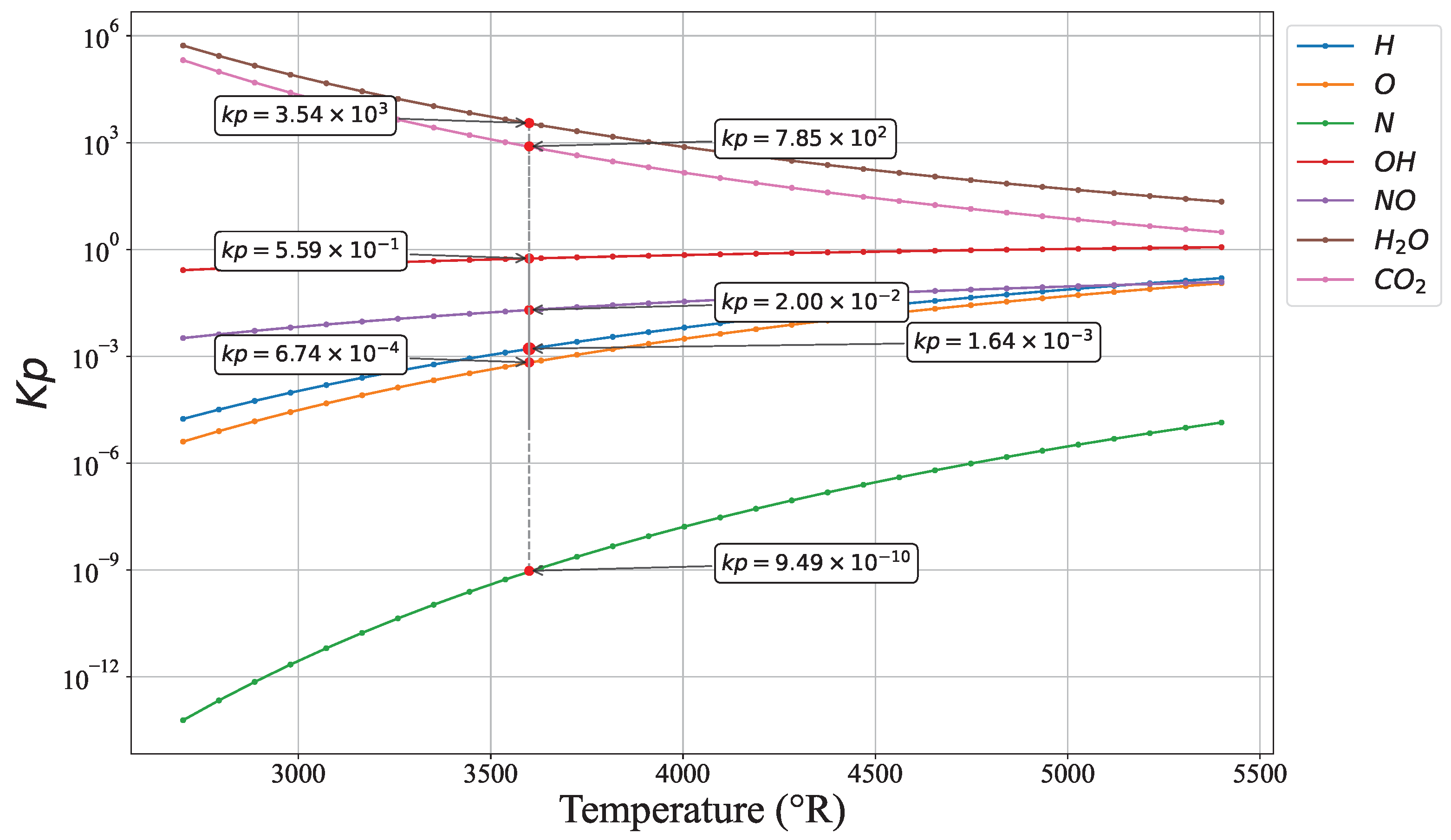
Gas Equilibrium Constants
2.3. Numerical Modeling of the Combustion Process
Initial Value Estimation
3. Results
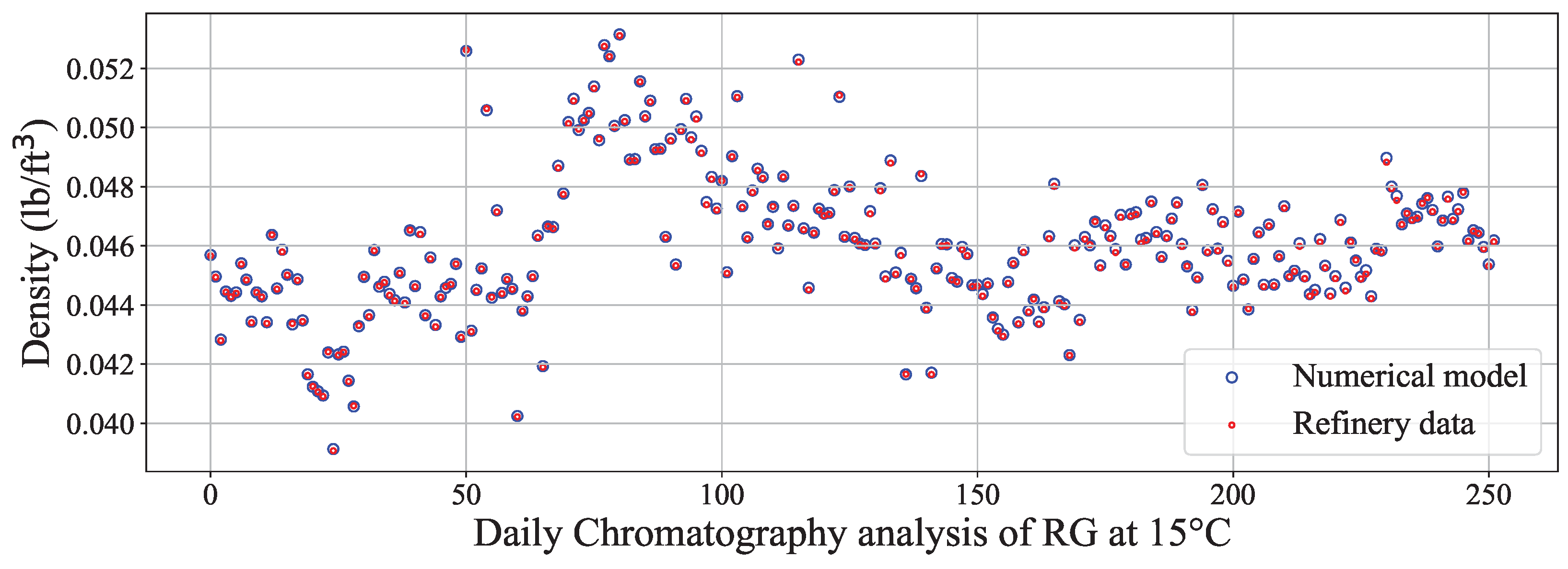
3.1. Numerical Model Validation
3.2. Approaches for Achieving a 50%+ Reduction in LPG Use
- Calculate the mass and density of the gas mixture.
- The LHV of the mixture must be .
- Obtain the adiabatic flame temperature.
- Reducing emissions and minimizing excess air.
4. Conclusions
Author Contributions
Funding
Data Availability Statement
Acknowledgments
Conflicts of Interest
References
- Garg, A. A New Approach to Optimizing Fired Heaters. 2010. Available online: https://oaktrust.library.tamu.edu/handle/1969.1/94037 (accessed on 19 September 2024).
- Garg, A. Optimize fired heater operations to save money. Hydrocarb. Process. 1997, 76, 97–112. [Google Scholar]
- Litvinenko, V. The role of hydrocarbons in the global energy agenda: The focus on liquefied natural gas. Resources 2020, 9, 59. [Google Scholar] [CrossRef]
- Filimonova, I.V.; Cherepanova, D.; Provornaya, I.; Kozhevin, V.; Nemov, V. The dependence of sustainable economic growth on the complex of factors in hydrocarbons-exporting countries. Energy Rep. 2020, 6, 68–73. [Google Scholar] [CrossRef]
- Tcvetkov, P.; Cherepovitsyn, A.; Makhovikov, A. Economic assessment of heat and power generation from small-scale liquefied natural gas in Russia. Energy Rep. 2020, 6, 391–402. [Google Scholar] [CrossRef]
- Garba, M.D.; Usman, M.; Khan, S.; Shehzad, F.; Galadima, A.; Ehsan, M.F.; Ghanem, A.S.; Humayun, M. CO2 towards fuels: A review of catalytic conversion of carbon dioxide to hydrocarbons. J. Environ. Chem. Eng. 2021, 9, 104756. [Google Scholar] [CrossRef]
- Miller, S.A.; Wilkinson, J.D.; Lynch, J.T.; Hudson, H.M.; Cuellar, K.T.; Johnke, A.F.; Lewis, W.L. Hydrocarbon Gas Processing. U.S. Patent 10,227,273, 12 March 2019. [Google Scholar]
- Qamar, R.A.; Mushtaq, A.; Ulla, A.; Ali, Z.U. Simulation of Liquefied Petroleum Gas Recovery from Off Gases in a Fuel Oil Refinery. J. Adv. Res. Fluid Mech. Therm. Sci. 2020, 73, 109–130. [Google Scholar] [CrossRef]
- Eshaghi, S.; Hamrang, F. An innovative techno-economic analysis for the selection of an integrated ejector system in the flare gas recovery of a refinery plant. Energy 2021, 228, 120594. [Google Scholar] [CrossRef]
- Cala, O.M.; Stand, L.M.; Kafarov, V.; Rueda, J.S. Efecto de la composición del gas de refinería sobre las características del proceso de combustión. Rev. Ing. Univ. Medellín 2013, 12, 101–111. [Google Scholar] [CrossRef]
- Arefin, M.A.; Nabi, M.N.; Akram, M.W.; Islam, M.T.; Chowdhury, M.W. A review on liquefied natural gas as fuels for dual fuel engines: Opportunities, challenges and responses. Energies 2020, 13, 6127. [Google Scholar] [CrossRef]
- Amell, A.; Barraza, L.; Gómez, E. Tecnología de la Combustión de Gases y Quemadores Atmosféricos de Premezcla. Línea, Disponible. 1996. Available online: http://es.scribd.com/doc/73707395/3-Quemadores-Atmosfericos-1 (accessed on 19 September 2024).
- Murshed, M.; Alam, R.; Ansarin, A. The environmental Kuznets curve hypothesis for Bangladesh: The importance of natural gas, liquefied petroleum gas, and hydropower consumption. Environ. Sci. Pollut. Res. 2021, 28, 17208–17227. [Google Scholar] [CrossRef]
- Kim, S.Y.; Costa, A.L.; Bagajewicz, M.J. New robust approach for the globally optimal design of fired heaters. Chem. Eng. Res. Des. 2023, 197, 434–448. [Google Scholar] [CrossRef]
- Ghorashi, S.A.; Khandelwal, B. Toward the ultra-clean and highly efficient biomass-fired heaters. A review. Renew. Energy 2023, 205, 631–647. [Google Scholar] [CrossRef]
- Qasim, F.; Lee, D.H.; Won, J.; Ha, J.K.; Park, S.J. Development of Advanced Advisory System for Anomalies (AAA) to Predict and Detect the Abnormal Operation in Fired Heaters for Real Time Process Safety and Optimization. Energies 2021, 14, 7183. [Google Scholar] [CrossRef]
- Thorat, S.; McQueen, G.; Luzunaris, P.T. The role of optimal design and application of heat tracing systems to improve the energy conservation in petrochemical facilities. IEEE Trans. Ind. Appl. 2013, 50, 163–173. [Google Scholar] [CrossRef]
- Masoumi, M.E.; Izakmehri, Z. Improving of refinery furnaces efficiency using mathematical modeling. Int. J. Model. Optim. 2011, 1, 74. [Google Scholar] [CrossRef]
- EU. A Clean Planet for All, a European Long-Term Strategic Vision for a Prosperous, Modern, Competitive and Climate Neutral Economy; Depth Analysis in Support of the Commission Communication Com; European Commission: Brussels, Belgium, 2018; Volume 773. [Google Scholar]
- Wildy, F.; Instruments, A.P. Fired heater optimization. In Technical Sales Support Manager; AMETEK Process Instruments: Pittsburgh, PA, USA, 2000. [Google Scholar]
- Rico, J.C.S.; Sánchez, Y.A.C. Análisis teórico de la combustión en quemadores de gas natural. Sci. Tech. 2005, 3, 139–143. [Google Scholar]
- Bouras, F.; Khaldi, F. Optimization of Combustion Efficiency Using a Fuel Composition Based on CH4 and/or H2. Russ. J. Appl. Chem. 2020, 93, 1954–1959. [Google Scholar] [CrossRef]
- Horbaj, P. Simulation method for optimization of a mixture of fuel gases. Gas Waerme Int. 2000, 49, 250–252. [Google Scholar]
- Kazi, S.R.; Sundar, K.; Srinivasan, S.; Zlotnik, A. Modeling and optimization of steady flow of natural gas and hydrogen mixtures in pipeline networks. Int. J. Hydrogen Energy 2024, 54, 14–24. [Google Scholar] [CrossRef]
- Simsek, S.; Uslu, S.; Simsek, H.; Uslu, G. Improving the combustion process by determining the optimum percentage of liquefied petroleum gas (LPG) via response surface methodology (RSM) in a spark ignition (SI) engine running on gasoline-LPG blends. Fuel Process. Technol. 2021, 221, 106947. [Google Scholar] [CrossRef]
- Derikvand, H.; Dehaj, M.S.; Taghavifar, H. The effect of different sampling method integrated in NSGA II optimization on performance and emission of diesel/hydrogen dual-fuel CI engine. Appl. Soft Comput. 2022, 128, 109434. [Google Scholar] [CrossRef]
- Saifullin, E.; Larionov, V.; Busarov, A.; Busarov, V. Optimization of hydrocarbon fuels combustion variable composition in thermal power plants. J. Phys. Conf. Ser. 2016, 669, 012037. [Google Scholar] [CrossRef]
- Patrón, G.D.; Ricardez-Sandoval, L. An integrated real-time optimization, control, and estimation scheme for post-combustion CO2 capture. Appl. Energy 2022, 308, 118302. [Google Scholar] [CrossRef]
- Cote Florez, M.S. Revision de Alternativas Operativas Para el Cumplimiento de Especificaciones de Calidad de Gas en un Campo Productor. Ph.D. Thesis, Universidad Industrial de Santander, Escuela De Ingeniería de Petróleos, Bucaramanga, Colombia, 2018. [Google Scholar]
- Arroyo, H.; Nichiren, S.; Alonso, M.; Delfin, F. Calidad y Medición del Gas Natural. 2006. Available online: https://es.scribd.com/document/462864821/Calidad-y-medicion-del-gas-natural (accessed on 19 September 2024).
- Chomiak, J.; Longwell, J.; Sarofim, A. Combustion of low calorific value gases; problems and prospects. Prog. Energy Combust. Sci. 1989, 15, 109–129. [Google Scholar] [CrossRef]
- Pinzón Vargas, B.L.; Plazas Puentes, M.I. Evaluación Técnico-Financiera de las Tecnologías de Construcción Modular para la Refinación de Petróleo Crudo en el Proyecto RefiBoyacá. Bachelor’s Thesis, Fundación Universidad de América, Bogotá, Colombia, 2018. [Google Scholar]
- Qin, C.; Li, J.; Yang, C.; Ai, B.; Zhou, Y. Comparative Study of Parameter Extraction from a Solar Cell or a Photovoltaic Module by Combining Metaheuristic Algorithms with Different Simulation Current Calculation Methods. Energies 2024, 17, 2284. [Google Scholar] [CrossRef]
- Olikara, C.; Borman, G.L. A Computer Program for Calculating Properties of Equilibrium Combustion Products with Some Applications to IC Engines; Technical Report; SAE Technical Paper; SAE International: Warrendale, PA, USA, 1975. [Google Scholar]
- Lide, D.R. CRC Handbook of Chemistry and Physics; CRC Press: Boca Raton, FL, USA, 2004; Volume 85. [Google Scholar]
- Turns, S.R. Introdução à Combustão-: Conceitos e Aplicações; AMGH Editora: Porto Alegre, Brazil, 2013. [Google Scholar]
- Worters, M.; Millard, D.; Hunter, G.; Helling, C.; Woitke, P. Comparison Catalogue of Gas-Equilibrium Constants, Kp. 2017. Available online: https://research-repository.st-andrews.ac.uk/handle/10023/12242 (accessed on 19 September 2024).
- Klotz, I.M. Chemical Thermodynamics; WA Benjamin Inc.: New York, NY, USA, 1964. [Google Scholar]
- Yıldız, M. Chemical equilibrium based combustion model to evaluate the effects of H2 addition to biogases with different CO2 contents. Int. J. Hydrogen Energy 2024, 52, 1334–1344. [Google Scholar] [CrossRef]
- Way, R. Methods for determination of composition and thermodynamic properties of combustion products for internal combustion engine calculations. Proc. Inst. Mech. Eng. 1976, 190, 687–697. [Google Scholar] [CrossRef]


| Fuels | |||||
|---|---|---|---|---|---|
| Comp. | MF | MF | MF | MF | MF |
| 0.16983526 | 0.28839122 | 0.15382659 | 0.0 | 0.0 | |
| 0.00355668 | 0.0018357 | 0.00180876 | 0.0 | 0.0 | |
| 0.50036226 | 0.49431918 | 0.63173331 | 0.9831 | 0.0 | |
| 0.1371265 | 0.04462025 | 0.11880152 | 0.00258124 | 0.9838 | |
| 0.05565108 | 0.03992771 | 0.04821289 | 0.0 | 0.0 | |
| 0.0549727 | 0.0147482 | 0.00479593 | 0.002 | 0.0054 | |
| propylene | 0.02094179 | 0.00305931 | 0.00649243 | 0.0 | 0.0098 |
| 0.0 | 0.0 | 0.00327537 | 0.0 | 0.001 | |
| 7.54 | 0.0 | 6.62 | 0.0 | 0.0 | |
| isobutane | 0.00558021 | 0.004937739 | 0.00230704 | 0.0 | 0.0 |
| propadiene | 0.0 | 0.0 | 0.0 | 0.0 | 0.0 |
| n-butane | 0.00679208 | 0.00343208 | 0.00306676 | 0.0 | 0.0 |
| 0.0004077 | 0.0153073 | 0.00022166 | 0.001 | 0.0 | |
| trans-2-butene | 0.0032849 | 0.0023618 | 0.0013005 | 0.0 | 0.0 |
| 0.0212296 | 0.080129 | 0.0109625 | 0.011 | 0.0 | |
| 1-butene | 0.0032146 | 0.00032 | 0.0010858 | 0.0 | 0.0 |
| isobutene | 0.0042796 | 0.0008848 | 0.0009842 | 0.0 | 0.0 |
| 2-butene | 0.0022651 | 0.0015048 | 1.32 | 0.0 | 0.0 |
| isopentene | 0.0020144 | 0.000221 | 0.0022329 | 0.0002048 | 0.0 |
| n-pentane | 0.00162679 | 5.559 | 0.0021111 | 6.879 | 0.0 |
| 1,3-butadiene | 0.0001166 | 0.0 | 4.06 | 0.0 | 0.0 |
| 0.00653259 | 0.0039111 | 0.0067198 | 0.0 | 0.0 | |
| Hexans+ | 0.0002015 | 3.27 | 0.0 | 3.03 | 0.0 |
| 0.9999994 | 0.99999949 | 0.99999948 | 0.99998514 | 1.0 |
| Equation | A | B | C | D | E |
|---|---|---|---|---|---|
| (10) | −0.112464 × | 0.267269 × | −0.7457 × | 0.242484 × | |
| (11) | −0.129540 × | 0.321779 × | −0.7383 × | 0.344645 × | |
| (12) | −0.245828 × | 0.314505 × | −0.9637 × | 0.585643 × | |
| (13) | −0.213308 × | 0.355015 × | −0.3102 × | ||
| (14) | 0.150879 × | −0.470959 × | 0.272805 × | −0.1544 × | |
| (15) | 0.124210 × | −0.260286 × | −0.1626 × | ||
| (16) | −0.4153 × | 0.148627 × | −0.475746 × | −0.9002 × |
| Gas | Mass | Density | Density | LHV |
|---|---|---|---|---|
| gmol | kg/m3 | lb/ft3 | BTU/ft3 | |
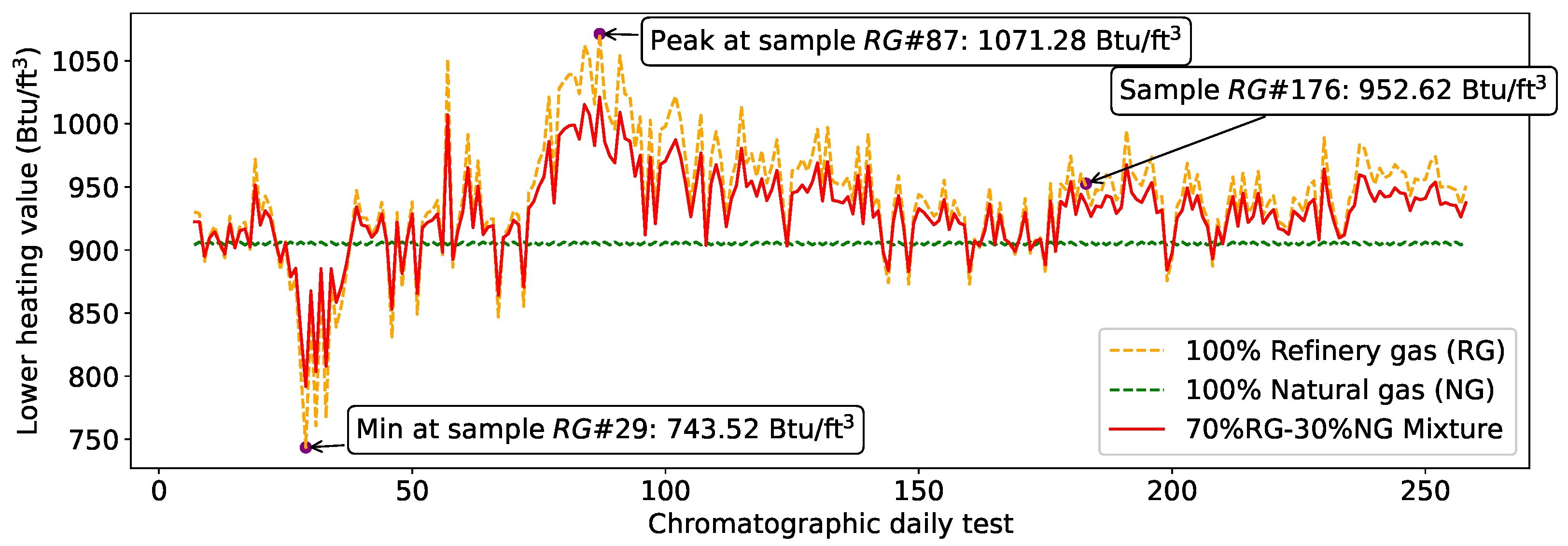
| 15.48 | 0.6558 | 0.04094 | 743.52 | |
| 20.06 | 0.8513 | 0.05314 | 1071.28 | |
| 17.38 | 0.7371 | 0.04601 | 952.62 | |
| 16.29 | 0.6907 | 0.04311 | 903.98 | |
| 44.23 | 1.9040 | 0.11886 | 2225.47 |
| Mix | RG-NG-LPG | Mass | Density | LHV |
|---|---|---|---|---|
| %-%-% | gmol | lb/ft3 | Btu/ft3 | |
| 70-14-16 | 20.19 | 0.0537 | 1003.09 | |
| 70-30-00 | 18.92 | 0.0501 | 1021.09 | |
| 70-25-05 | 18.45 | 0.0489 | 1004.10 |
| Comb. | ||||
|---|---|---|---|---|
| Prod. | MF | MF | MF | |
| H | ||||
| O | ||||
| N | ||||
| SUM |
Disclaimer/Publisher’s Note: The statements, opinions and data contained in all publications are solely those of the individual author(s) and contributor(s) and not of MDPI and/or the editor(s). MDPI and/or the editor(s) disclaim responsibility for any injury to people or property resulting from any ideas, methods, instructions or products referred to in the content. |
© 2024 by the authors. Licensee MDPI, Basel, Switzerland. This article is an open access article distributed under the terms and conditions of the Creative Commons Attribution (CC BY) license (https://creativecommons.org/licenses/by/4.0/).
Share and Cite
Sánchez, R.; Palencia-Díaz, A.; Fábregas-Villegas, J.; Velilla-Díaz, W. Fired Heaters Optimization by Estimating Real-Time Combustion Products Using Numerical Methods. Energies 2024, 17, 6190. https://doi.org/10.3390/en17236190
Sánchez R, Palencia-Díaz A, Fábregas-Villegas J, Velilla-Díaz W. Fired Heaters Optimization by Estimating Real-Time Combustion Products Using Numerical Methods. Energies. 2024; 17(23):6190. https://doi.org/10.3390/en17236190
Chicago/Turabian StyleSánchez, Ricardo, Argemiro Palencia-Díaz, Jonathan Fábregas-Villegas, and Wilmer Velilla-Díaz. 2024. "Fired Heaters Optimization by Estimating Real-Time Combustion Products Using Numerical Methods" Energies 17, no. 23: 6190. https://doi.org/10.3390/en17236190
APA StyleSánchez, R., Palencia-Díaz, A., Fábregas-Villegas, J., & Velilla-Díaz, W. (2024). Fired Heaters Optimization by Estimating Real-Time Combustion Products Using Numerical Methods. Energies, 17(23), 6190. https://doi.org/10.3390/en17236190