AVR Fractional-Order Controller Based on Caputo–Fabrizio Fractional Derivatives and Integral Operators

Abstract

The application of a fractional-order controller (FOC) using the Caputo–Fabrizio representation in the automatic voltage regulation (AVR) system of a synchronous generator is shown in this paper. The mathematical model of the system is created and the adequacy of the model is confirmed. The efficiency of the proposed regulator in different operating regimes is demonstrated. In particular, the proposed controller improves voltage regulation in a wide range of changes in the coordinates that characterize the power system operation mode, and it increases the system’s robustness to both uncertainties and nonlinearities that often occur in power systems. The synthesized fractional-order regulator provides higher response and control accuracy compared to traditional regulators used in automatic voltage regulation (AVR) systems.

1. Introduction

In the 21st century, humanity is faced with a new challenge—the need to radically reduce greenhouse gas emissions. Satisfying the projected electricity demand in 2050 will require the use of various low- or zero-carbon technologies, including nuclear power as a distributed low-carbon technology [1]. Nuclear power remains a strong competitor as a supplier of carbon-neutral electric power for a base load. Small nuclear modular reactors (SMRs) offer a variety of advantages, including lower capital costs, enhanced safety and greater flexibility [2]. SMRs are seen as a promising technology that can simultaneously satisfy the demand for electricity and heat [3], which would significantly increase the energy independence of communities, and provide a reliable source of clean energy production.

In a dispersed power generation system, SMRs can be used in connection with renewable energy sources to create hybrid power systems. The growing impact of renewable energy sources require greater system flexibility to always keep supply and demand in balance [4,5]. In such hybrid systems, SMRs can be used as a stable and reliable power source, as well as to balance grid-load oscillations caused by the specific operation of the renewable energy sources [6]. The operational stability of such hybrid networks is directly related to the quality of the SMR control, including synchronous generator excitation control. At the same time, many publications on SMR control do not attend to the synchronous generator control, supposing that traditional excitation control systems will be used.

The problem of synchronous generator control-system synthesis is not new [7,8,9]. In [10], a review of the proposed approaches to the synthesis of power system control systems is presented, including decentralized and distributed controls, which are becoming the most popular in distributed generation systems and smart grids. To strengthen the damping and improve system stability, automatic voltage regulation and power system stabilization (AVR/PSS) systems are widely used in existing power systems [11,12]. Since AVR/PSS are traditionally synthesized separately (AVR is the main controller, PSS is an additional or slave controller), effective voltage control and system stability improvements are difficult to achieve simultaneously [8,12]. In addition, controllers synthesized on the basis of linearized models of power systems that correspond to certain operating conditions considerably worsen the control quality when operating conditions change [13]. To avoid these problems, the Lyapunov method was used in [12] to synthesize controllers, which ensures the stability of the system under parameter changes, and the application of the sliding mode control method was proposed in [14,15,16]. Synchronous generator excitation controllers synthesized by the sliding mode control method are usually used to improve the transient stability of power systems. The main problem of sliding mode control is the well-known oscillation effects that can excite the nonmodeled dynamics of a synchronous generator and usually occur as vibrations in the mechanical part, which leads to a decrease in control efficiency.

Nonlinear controllers of synchronous generator excitation control systems synthesized based on nonlinear models by applying modern methods of nonlinear control theory successfully eliminate the limitations that are typical in such systems, synthesized by methods of classical control theory. In [17,18,19], the application of energy-based approaches, in particular the theory of passivity control, to the synthesis of control systems for a stand-alone generator of an autonomous power system with an energy storage device and a small modular reactor circuit are proposed. The main problem with this approach is the choice of the interaction and damping matrices, as well as the synthesis of their parameters. In [20,21,22], adaptive controllers for excitation control systems synthesized by the back-stepping method were proposed. The results presented by the authors demonstrate the reliable operation of the system under parametric uncertainty, provided that the adaptation coefficient is properly selected and the Lyapunov control functions are formed. Another approach that has been widely applied in recent years in power systems is model predictive control [23,24,25]. As noted in [25], the main feature of a control system synthesized in this way is to provide stability to non-simulated power system dynamics. The main disadvantages of such systems are the dependence of the control quality on the horizon of the prediction and the complexity of the system, due to the demand to obtain information that cannot be measured directly. A similar problem with obtaining information about variables that cannot be measured directly occurs in excitation control systems synthesized by the feedback linearization method [26,27,28,29,30]. Synthesized by feedback linearization, excitation controllers are used to improve the transient stability of power systems and provide it in a significantly better way than other nonlinear control technologies [29]. However, the implementation of such controllers for excitation control systems requires the estimation of the rotor angle, which leads to system complexity. In [28,30], a partial feedback linearization control was proposed, which utilizes the speed deviation rather than the rotor angle as feedback. Since the speed deviation is a derivative of the rotor angle, the partial feedback linearization control provides higher damping in the system in comparison to other excitation controllers synthesized by the feedback linearization method. A significant disadvantage of such systems is still their robustness to large external disturbances and parameter uncertainties. Meanwhile, the implementation of robust control methods [31] is complicated by the nonlinearity of the object, and requires the use of local linearization and solving the Riccati equation at each control step.

It is important to note that the excitation control systems analyzed above, based on nonlinear control theory, are quite complex and may be difficult to implement in real systems.

The efficiency of the proposed control systems is traditionally analyzed using mathematical models. Depending on the research objectives, two approaches are used [32,33]:

-

A synchronous generator operates in a self-contained mode (the power system is replaced by an infinite bus);

-

The synchronous generator operates as part of a system (a multi-machine model of the system, which enables the analysis of the interactions between generators operating in this system).

Mathematical models of a synchronous generator in the form of transfer functions of 3–5 orders in the system model “synchronous generator-infinite bus” are useful for the synthesis of control influences, analysis of small-scale stability and system robustness under different operating modes [34]. Modern power systems are mostly interconnected in nature, so it is important to create an appropriate representation of an interconnected power system to conduct research on such multi-machine power systems. Until recently, the multi-machine representation was formed based on two-machine models and also used a description in the form of transfer functions typical of the synchronous generator-infinite bus model. At the present time, models that considered both the processes in the damping windings and the mutual influences between generators in different operating modes were used. The increasing number of machine models in a multi-machine system leads to a more complex system model, which makes it difficult to synthesize control influences and understand the physical processes in the system. Moreover, physical understanding becomes fuzzy when we deal with multiple machines. The system model description in the form of transfer functions does not take into account the nonlinear dynamics of the system [35] and the change in parameters during its operation. The imperfection of the models used in the synthesis of control influences can cause incorrect operation of the control system in real conditions. The analysis of processes in hybrid systems [36,37,38] requires the use of more complex nonlinear models of synchronous generators [39], including those that can operate in real-time systems and be used to set up excitation control systems [40].

Thus, a significant range of disturbance changes and the rapidity of processes in distributed power systems with different energy sources complicate the task of generator control and motivates the search for new approaches to excitation control that would improve the quality of voltage regulation and generator stability under such conditions [6,41]. In this case, as mentioned above, for the synthesis of control systems, it is necessary to use models of multi-machine systems that take into account the nonlinearity and mutual influences between all elements. In our opinion, a perspective approach to solving the above-mentioned problems is to use fractional calculus. The use of this approach demonstrates successful results both for system modeling [42,43] and for the synthesis of control influences [44,45,46].

The novelty of this study is the proposed new structure of the synchronous generator’s automatic voltage regulation system with a fractional-order controller. The synthesis of the proposed fractional-order controller is described in Section 1. Section 2 describes the developed mathematical model created using the original method of average voltages in numerical integration step (AVIS), which was used to verify the effectiveness of the proposed controller. In Section 3, the adequacy of the developed model is confirmed by comparing the results of mathematical modelling with experimental data obtained at the power plant. Section 4 presents the results of mathematical modelling, which confirm the effectiveness of the proposed control system in comparison with the classical control system in a two-bus system with consideration of mutual influences between generators.

• Proportional–integral–differential (PID) fractional-order controller

The equation of the fractional-order PID controller is as follows [47]:

$$u\left(t\right)=k_p·e\left(t\right)+k_i·I^{\mu }e\left(t\right)+k_d·D^{\alpha }e\left(t\right),$$

(1)

where e(t) is the regulation error; k_p, k_i, k_d are the gain of the proportional, integral and differential components, respectively.

Traditionally, the Caputo representation has been used to describe the fractional order derivative D^α (α ∈ R⁺) of function g(t):

$${}^{C}D^{\alpha }g\left(t\right)={\displaystyle \frac{1}{\Gamma \left(1-\alpha \right)}}·{{\displaystyle \int }}_0^t{\left(t-\tau \right)}^{-\alpha }·\dot{g}\left(\tau \right)d\tau ,$$

(2)

and the Riemann–Liouville representation is used to describe the fractional order integral ^RLI^α of function g(t):

$${}^{RL}I^{\alpha }g\left(t\right)={\displaystyle \frac{1}{\Gamma \left(\alpha \right)}}·{{\displaystyle \int }}_0^t{\left(t-\tau \right)}^{\alpha -1}·g\left(\tau \right)d\tau ,$$

(3)

where Γ is the gamma function.

In the analysis and synthesis of control systems, it is often assumed that the initial conditions of the differential equations of the automatic control system equal zero. Under this assumption, the time-domain operator D^α can be simply represented in the frequency domain as s^α. In this context, the negative sign in the derivative order (−α) essentially means a fractional integration operator [48]. Subsequently, the Oustaloup approximation is used to approximate the fractional derivative s^γ at 0 < α < 1 with an integer operator [49]. As noted in [50], the use of this approach causes certain difficulties both at the stage of synthesis of control influences and in the analysis of systems in the time domain.

In [51], Caputo and Fabrizio proposed a representation of the fractional derivative of order 0 < α < 1 by the following equation:

$${}^{CF}D^{\alpha }g\left(t\right)={\displaystyle \frac{\left(2-\alpha \right)·M\left(\alpha \right)}{2·\left(1-\alpha \right)}}·{{\displaystyle \int }}_0^t{e}^{{\displaystyle \frac{-\alpha \left(t-\tau \right)}{1-\alpha }}}·\dot{g}\left(\tau \right)d\tau ,$$

(4)

obtained from the Caputo view by replacing the Kernel ${\left(t-\tau \right)}^{-\alpha }$ by $e^{{\displaystyle \frac{-\alpha \left(t-\tau \right)}{1-\alpha }}}$, and 1/Γ(α) on ${\displaystyle \raisebox{1ex}{$1$}\!\left/ \!\raisebox{-1ex}{$\sqrt{2\pi \left(1-{\alpha }^2\right)}$}\right.}$; at the same time, $M\left(\alpha \right)={\displaystyle \raisebox{1ex}{$2$}\!\left/ \!\raisebox{-1ex}{$\left(2-\alpha \right)$}\right.}$ is a normalization factor that depends on α. Then the representation of the fractional derivative of the order 0 < α < 1 will be as shown in [52]:

$${}^{CF}D^{\alpha }g\left(t\right)={\displaystyle \frac{1}{\left(1-\alpha \right)}}{{\displaystyle \int }}_0^t{e}^{{\displaystyle \frac{-\alpha \left(t-\tau \right)}{1-\alpha }}}·\dot{g}\left(\tau \right)d\tau .,$$

(5)

The fractional integral can be represented as follows [53]:

$${}^{CF}I^{\alpha }g\left(t\right)={\displaystyle \frac{1}{\alpha }}{{\displaystyle \int }}_0^t{e}^{{\displaystyle \frac{-\left(1-\alpha \right)·\left(t-\tau \right)}{\alpha }}}g\left(\tau \right)d\tau ,$$

(6)

After applying the Laplace transform with the assumption of zero initial conditions, we obtain:

$$\mathcal{L}({}^{CF}D^{\alpha }g\left(t\right))={\displaystyle \frac{1}{1-\alpha }}·{\displaystyle \frac{s·G\left(s\right)}{s+\frac{\alpha }{1-\alpha }}}={\displaystyle \frac{\frac{1}{\alpha }·s}{s·\frac{1-\alpha }{\alpha }+1}}G\left(s\right),$$

(7)

$$\mathcal{L}({}^{CF}I^{\alpha }g\left(t\right))={\displaystyle \frac{1}{\alpha }}·{\displaystyle \frac{1}{s+\frac{1-\alpha }{\alpha }}}G\left(s\right)={\displaystyle \frac{\frac{1}{1-\alpha }}{\frac{\alpha }{1-\alpha }s+1}}G\left(s\right),$$

(8)

The use of the Caputo–Fabrizio representation makes it possible to obtain Laplace transform integer representations of the derivative and fractional integral, which avoids the approximation of the fractional representation of the derivative s^α and the integral s^−α and, accordingly, the PID controller equation can be written as follows:

$$u\left(s\right)=k_p·e\left(s\right)+{\displaystyle \frac{k_i}{\mu ·s+\left(1-\mu \right)}}e\left(s\right)+{\displaystyle \frac{\frac{k_d}{\alpha }s}{\frac{1-\alpha }{\alpha }s+1}}e\left(s\right),$$

(9)

This structure of the controller, with a change in the parameter μ, makes it possible to implement various structures of excitation control systems [54]. In particular, for the case 0 < μ < 1, taking $T_{f1}={\displaystyle \frac{1-\alpha }{\alpha }};T_{f2}={\displaystyle \frac{\mu }{1-\mu }}$ we obtained the following:

$$\begin{array}{l}u\left(s\right)=K_P+{\displaystyle \frac{\frac{K_D}{\alpha }s}{T_{f1}s+1}}+{\displaystyle \frac{\frac{K_I}{1-\mu }}{T_{f2}s+1}}={\displaystyle \frac{\left[K_P(T_{f1}{T}_{f2}{s}^2+\left(T_{f1}+T_{f2}\right)s+1)+\frac{K_D}{\alpha }s\left(T_{f2}s+1\right)+\frac{K_I}{1-\mu }\left(T_{f1}s+1\right)\right]}{\left(T_{f1}s+1\right)\left(T_{f2}s+1\right)}}=\\ ={\displaystyle \frac{s^2(K_P{T}_{f1}{T}_{f2}+\frac{K_D}{\alpha }{T}_{f2})+s\left(K_P(T_{f1}+T_{f2}\right)+\frac{K_D}{\alpha }+\frac{K_I}{1-\mu }{T}_{f1})+K_P+\frac{K_I}{1-\mu }}{\left(T_{f1}s+1\right)\left(T_{f2}s+1\right)}}\end{array}$$

(10)

For

$$D=\left(K_P(T_{f1}+T_{f2}\right)+{\displaystyle \frac{K_D}{\alpha }}+{\displaystyle \frac{K_I}{1-\mu }}{T}_{f1}{)}^2-4(K_P{T}_{f1}{T}_{f2}+{\displaystyle \frac{K_D}{\alpha }}{T}_{f2})\left(K_P+{\displaystyle \frac{K_I}{1-\mu }}\right)\gg 0$$

$${\lambda }_{1,2}={\displaystyle \frac{-\left(K_P(T_{f1}+T_{f2}\right)+\frac{K_D}{\alpha }+\frac{K_I}{1-\mu }{T}_{f1})\pm \sqrt{D}}{2(K_P{T}_{f1}{T}_{f2}+\frac{K_D}{\alpha }{T}_{f2})}}.$$

the output signal of the controller will be as follows:

$$u\left(s\right)=k{\displaystyle \frac{\left(T_{f3}s+1\right)\left(T_{f4}s+1\right)}{\left(T_{f1}s+1\right)\left(T_{f2}s+1\right)}},$$

(11)

where

$$\begin{gathered} T_{f3}={\displaystyle \frac{2(K_P{T}_{f1}{T}_{f2}+\frac{K_D}{\alpha }{T}_{f2})}{\left(K_P(T_{f1}+T_{f2}\right)+\frac{K_D}{\alpha }+\frac{K_I}{1-\mu }{T}_{f1})-\sqrt{D}}};T_{f4}={\displaystyle \frac{2(K_P{T}_{f1}{T}_{f2}+\frac{K_D}{\alpha }{T}_{f2})}{\left(K_P(T_{f1}+T_{f2}\right)+\frac{K_D}{\alpha }+\frac{K_I}{1-\mu }{T}_{f1})+\sqrt{D}}}; \\ k={\displaystyle \frac{\left(K_P+\frac{K_I}{1-\mu }\right)}{(K_P{T}_{f1}{T}_{f2}+\frac{K_D}{\alpha }{T}_{f2})}} \end{gathered}$$

which corresponds to the lead–lag structure of the compensator. Moreover, changing the parameters α and μ enables not only the control of the location of the zeros and poles of the compensator, but also changing its gain.

In the case of μ = 1, we obtain the traditional structure of a PID controller with a real differentiator:

$$u\left(s\right)=k_p·e\left(s\right)+{\displaystyle \frac{k_i}{s}}·e\left(s\right)+{\displaystyle \frac{\frac{k_d}{\alpha }s}{\frac{1-\alpha }{\alpha }s+1}}·e\left(s\right),$$

(12)

With similarity to the classical, the PID controller can be written as follows:

$$u\left(s\right)=k_p\left(1+{\displaystyle \frac{1}{{\tau }_i^{*}s}}+{\displaystyle \frac{{\tau }_d^{*}s}{\frac{{\tau }_d^{*}}{N}s+1}}\right)e\left(s\right),$$

(13)

where ${\tau }_i^{*}={\displaystyle \frac{k_p}{k_i}} {\tau }_d^{*}={\displaystyle \frac{k_d}{\alpha ·k_p}}\mathrm{and} {\displaystyle \frac{1-\alpha }{\alpha }}={\displaystyle \frac{{\tau }_d^{*}}{N}}$, $\mathrm{N}=2÷20$ is mostly assumed equal 10.

And applying classical methods of tuning PID controllers, in particular, the following: Ziegler–Nichols; Chien, Hrones and Reswick; Tyreus–Luyben:

$$\left\{\begin{array}{l}{k}_p={\beta }_1·k_u\\ {\displaystyle \frac{k_p}{k_i}}={\beta }_2·T_u\\ {\displaystyle \frac{k_d}{\alpha k_p}}={\beta }_3·T_u\\ {\displaystyle \frac{1-\alpha }{\alpha }}={\displaystyle \frac{{\beta }_3}{N}}{T}_u\end{array}\right.,$$

where ${\mathsf{\beta }}_1, {\mathsf{\beta }}_2, {\mathsf{\beta }}_3$ are parameters that depend on the chosen method of tuning the PID controller; k_u and T_u are the gain of the proportional controller at which the system has unattenuated oscillations and the period of these oscillations, respectively.

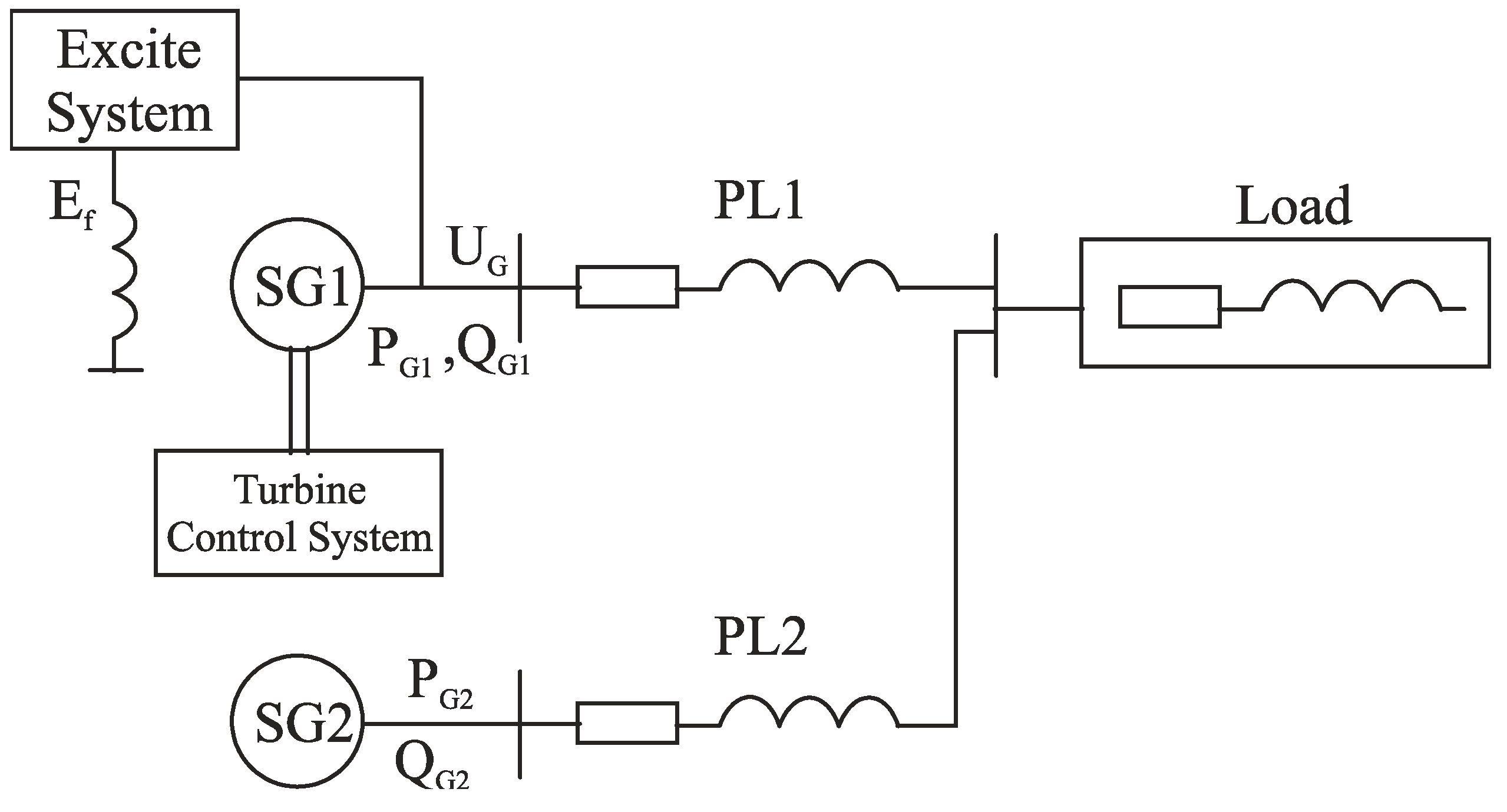
2. Mathematical Model of the Research System

The proposed generator voltage control system with fractional-order controller was studied for an example of a synchronous generator SG1 with a self-excitation system operating in a power system containing a parallel synchronous generator SG2 (the excitation system and turbine control system of this were assumed to be similar to SG1) and a load (Figure 1).

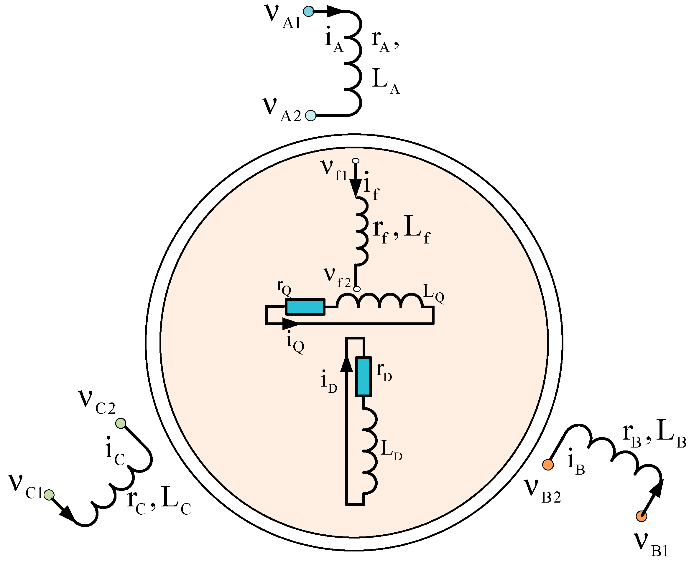
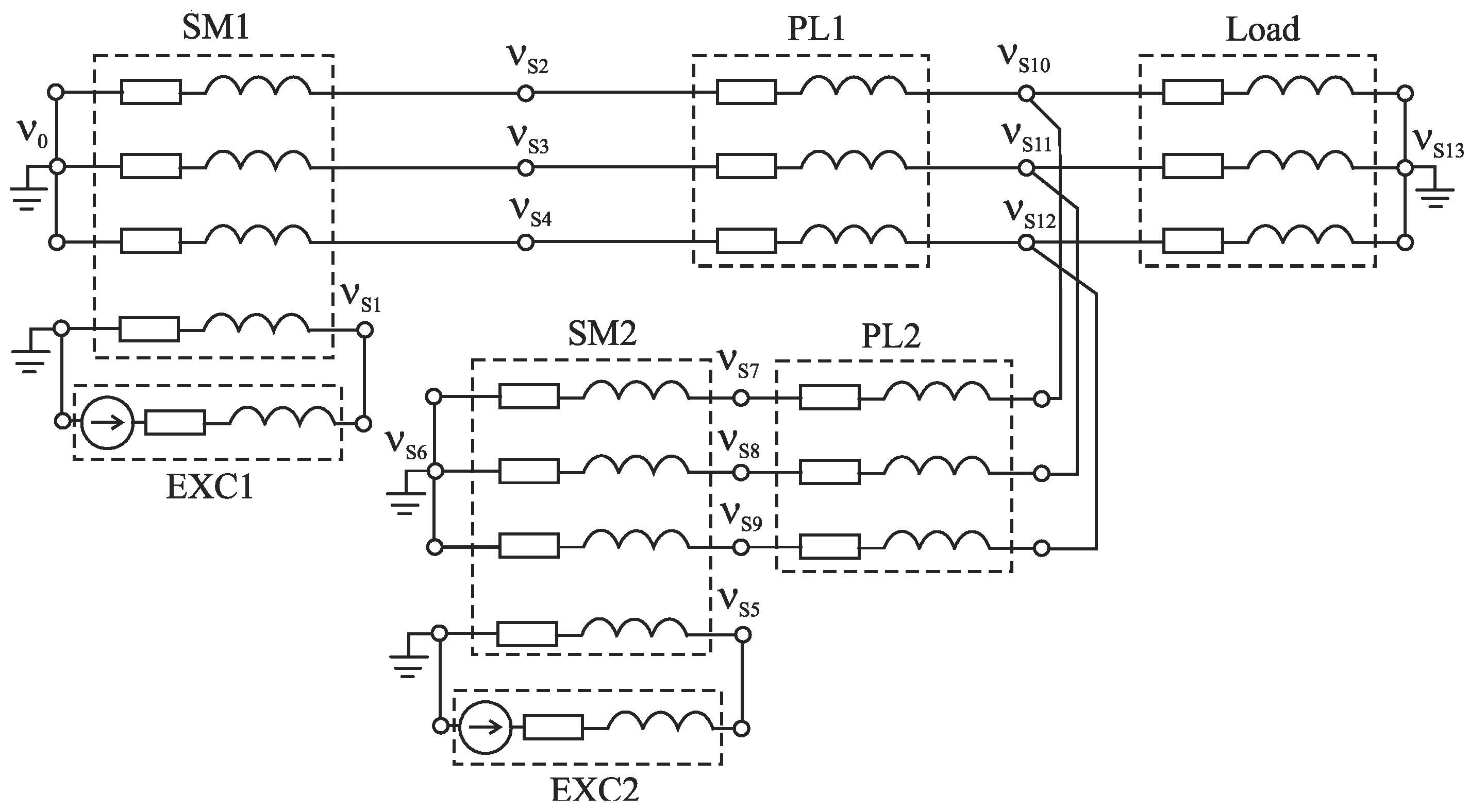
2.1. Mathematical Model of the Power Circuit

To create mathematical models of the elements of electric power systems, we used the method of average voltages in a numerical integration step (AVIS) described in [55]. According to this method, the following equation is written for an electrical branch containing a winding with active resistance R and inductance, capacitance C, and a source of EMF [55]:

$$\begin{gathered} \mathrm{U}+\mathrm{E}-{\mathrm{u}}_{\mathrm{R}0}-{\mathrm{u}}_{\mathrm{C}0}+\left({\displaystyle \frac{\mathrm{R}}{\mathrm{m}+1}}+{\displaystyle \frac{\Delta \mathrm{t}}{\mathrm{C}}}·{\displaystyle \frac{2-\left(\mathrm{m}+1\right)\left(\mathrm{m}+2\right)}{2\left(\mathrm{m}+1\right)\left(\mathrm{m}+2\right)}}\right){\mathrm{i}}_0- \\ -{\displaystyle \sum _{\mathrm{k}=1}^{\mathrm{m}-1}\left(\frac{\mathrm{R}\Delta {\mathrm{t}}^{\mathrm{k}}}{\left(\mathrm{k}+1\right)!}·\frac{\mathrm{m}-\mathrm{k}}{\mathrm{m}+1}+\frac{\Delta {\mathrm{t}}^{\mathrm{k}+1}}{\mathrm{C}\left(\mathrm{k}+2\right)!}·\frac{\left(\mathrm{m}+1\right)\left(\mathrm{m}+2\right)-\left(\mathrm{k}+1\right)\left(\mathrm{k}+2\right)}{\left(\mathrm{m}+1\right)\left(\mathrm{m}+2\right)}\right)\frac{{\mathrm{d}}^{\left(\mathrm{k}\right)}{\mathrm{i}}_0}{\mathrm{d}{\mathrm{t}}^{\left(\mathrm{k}\right)}}-} \\ -\left({\displaystyle \frac{\mathrm{R}}{\mathrm{m}+1}}+{\displaystyle \frac{\Delta \mathrm{t}}{\mathrm{C}\left(\mathrm{m}+1\right)\left(\mathrm{m}+2\right)}}\right){\mathrm{i}}_1-{\displaystyle \frac{{\mathsf{\psi }}_1-{\mathsf{\psi }}_0}{\Delta \mathrm{t}}}=0, \end{gathered}$$

(14)

where $\mathrm{U}={\displaystyle \frac{1}{\Delta \mathrm{t}}}{\displaystyle \underset{{\mathrm{t}}_0}{\overset{{\mathrm{t}}_0+\Delta \mathrm{t}}{\int }}\mathrm{udt}}$, $\mathrm{E}={\displaystyle \frac{1}{\Delta \mathrm{t}}}{\displaystyle \underset{{\mathrm{t}}_0}{\overset{{\mathrm{t}}_0+\Delta \mathrm{t}}{\int }}\mathrm{edt}}$ are the average values of applied voltage and electromotive force on the integration step (u and e are intermediated value of ones); u_R0 and u_C0 are the voltages on resistance and capacitor at the beginning of the integration step; i₀ and i₁ is the current value at the beginning and at the end of the integration step; ψ₀ and ψ₁ are branch flux linkages at the beginning and at the end of the integration step, Δt is the integration step value; m is the order of polynomial by which a current is described in an integration step (the order of AVIS method).

The calculation schemes of a synchronous machine in the form of a multipole is shown in Figure 2. The stator windings are modeled in phase coordinates, and the damper winding is represented by short-circuited branches along the d-axis and q-axis, respectively.

Applying Equation (14) for the second order (m = 2) to the electrical circuit of phase A of the stator winding (Figure 2), we obtain the following equation:

$${\mathrm{U}}_{\mathrm{A}}-{\mathrm{R}}_{\mathrm{A}}{\mathrm{i}}_{\mathrm{A}0}+{\displaystyle \frac{{\mathrm{R}}_{\mathrm{A}}}{3}}\left({\mathrm{i}}_{\mathrm{A}0}-{\mathrm{i}}_{\mathrm{A}1}\right)-{\displaystyle \frac{\mathrm{R}\Delta \mathrm{t}}{6}}{\displaystyle \frac{\mathrm{d}{\mathrm{i}}_{\mathrm{A}0}}{\mathrm{d}\mathrm{t}}}+{\displaystyle \frac{{\mathsf{\psi }}_{\mathrm{A}0}-{\mathsf{\psi }}_{\mathrm{A}1}}{\Delta \mathrm{t}}}=0$$

(15)

where ${\mathrm{U}}_{\mathrm{A}}={\displaystyle \frac{1}{\Delta \mathrm{t}}}{\displaystyle \underset{{\mathrm{t}}_0}{\overset{{\mathrm{t}}_0+\Delta \mathrm{t}}{\int }}{\mathrm{u}}_{\mathrm{A}}\mathrm{dt}}$—is the average voltage applied to the circuit at the step of numerical integration (u_A is the instantaneous value of the voltage applied to the circuit); hereafter, the index 0 means the value of the variable at the start of the step, and the index 1 means the value of the variable at the end of the step. Similar equations can be written for other circuits of the calculation scheme.

The phase linkage in Equation (15) is determined on the basis of the currents of all phases and windings of the SM (including damping windings), self and mutual inductances:

$${\mathsf{\psi }}_{\mathrm{A}}={\mathrm{L}}_{\mathrm{A}\mathrm{A}}{\mathrm{i}}_{\mathrm{A}}+{\mathrm{L}}_{\mathrm{A}\mathrm{B}}{\mathrm{i}}_{\mathrm{B}}+{\mathrm{L}}_{\mathrm{A}\mathrm{C}}{\mathrm{i}}_{\mathrm{C}}+{\mathrm{L}}_{\mathrm{A}\mathrm{F}}{\mathrm{i}}_{\mathrm{f}}+{\mathrm{L}}_{\mathrm{A}\mathrm{D}}{\mathrm{i}}_{\mathrm{D}}+{\mathrm{L}}_{\mathrm{A}\mathrm{Q}}{\mathrm{i}}_{\mathrm{Q}}.$$

(16)

The equations for flux linkages of other phases and windings will be similar.

Mark ${\overrightarrow{\mathrm{i}}}_{\mathrm{e}\mathrm{e}}={\left({\mathrm{i}}_{\mathrm{A}},{\mathrm{i}}_{\mathrm{B}},{\mathrm{i}}_{\mathrm{C}},{\mathrm{i}}_{\mathrm{f}}\right)}^{\mathrm{T}}$—column vector of external circuits (stator winding and excitation winding) currents; ${\overrightarrow{\mathrm{i}}}_{\mathrm{i}\mathrm{i}}={\left({\mathrm{i}}_{\mathrm{D}},{\mathrm{i}}_{\mathrm{Q}}\right)}^{\mathrm{T}}$—column vector of internal circuits (damping winding) currents; ${\overrightarrow{\mathsf{\nu }}}_1=\left({\mathsf{\nu }}_{\mathrm{A}1},{\mathsf{\nu }}_{\mathrm{B}1}\right.,{\mathsf{\nu }}_{\mathrm{C}1},{\left.{\mathsf{\nu }}_{\mathrm{f}1}\right)}^{\mathrm{T}}$, ${\overrightarrow{\mathsf{\nu }}}_2=\left({\mathsf{\nu }}_{\mathrm{A}2},{\mathsf{\nu }}_{\mathrm{B}2}\right.,{\mathsf{\nu }}_{\mathrm{C}2},{\left.{\mathsf{\nu }}_{\mathrm{f}2}\right)}^{\mathrm{T}}$ are the vectors of the external pole potentials; ${\overrightarrow{\mathsf{\psi }}}_{\mathrm{e}\mathrm{e}}=\left({\mathsf{\psi }}_{\mathrm{A}}\right.,{\mathsf{\psi }}_{\mathrm{B}},{\mathsf{\psi }}_{\mathrm{C}},{\left.{\mathsf{\psi }}_{\mathrm{f}}\right)}^{\mathrm{T}}$, $R_{\mathrm{e}\mathrm{e}}=\mathrm{diag}\left({\mathrm{r}}_{\mathrm{A}}\right.,{\mathrm{r}}_{\mathrm{B}},{\mathrm{r}}_{\mathrm{C}},\left.{\mathrm{r}}_{\mathrm{f}}\right)$ are the vectors of flux linkages and the matrices of the resistances for stator winding and excitation winding; ${\mathsf{\psi }}_{\mathrm{i}\mathrm{i}}={({\mathsf{\psi }}_{\mathrm{D}},{\mathsf{\psi }}_{\mathrm{Q}})}^{\mathrm{T}}$, $R_{\mathrm{i}\mathrm{i}}=\mathrm{diag}\left({\mathrm{r}}_{\mathrm{D}}\right.,\left.{\mathrm{r}}_{\mathrm{Q}}\right)$ are the vectors of flux linkages and the matrices of resistances of the damping winding.

Then, taking into account Equation (15), we can write the equation for the external circuits (stator and excitation windings)

$${\displaystyle \frac{1}{\Delta \mathrm{t}}}{\displaystyle \underset{{\mathrm{t}}_0}{\overset{{\mathrm{t}}_0+\Delta \mathrm{t}}{\int }}{\overrightarrow{\mathsf{\nu }}}_1\mathrm{d}\mathrm{t}}-{\displaystyle \frac{1}{\Delta \mathrm{t}}}{\displaystyle \underset{{\mathrm{t}}_0}{\overset{{\mathrm{t}}_0+\Delta \mathrm{t}}{\int }}{\overrightarrow{\mathsf{\nu }}}_2\mathrm{d}\mathrm{t}}-R_{\mathrm{e}\mathrm{e}}{\overrightarrow{\mathrm{i}}}_{\mathrm{e}\mathrm{e}0}+{\displaystyle \frac{R_{\mathrm{e}\mathrm{e}}}{3}}{\overrightarrow{\mathrm{i}}}_{\mathrm{e}\mathrm{e}0}-{\displaystyle \frac{R_{\mathrm{e}\mathrm{e}}}{3}}{\overrightarrow{\mathrm{i}}}_{\mathrm{e}\mathrm{e}1}-{\displaystyle \frac{R_{\mathrm{e}\mathrm{e}}\Delta \mathrm{t}}{6}}{\displaystyle \frac{\mathrm{d}{\overrightarrow{\mathrm{i}}}_{\mathrm{e}\mathrm{e}0}}{\mathrm{d}\mathrm{t}}}-{\displaystyle \frac{1}{\Delta \mathrm{t}}}\left({\overrightarrow{\mathsf{\psi }}}_{\mathrm{e}\mathrm{e}1}-{\overrightarrow{\mathsf{\psi }}}_{\mathrm{e}\mathrm{e}0}\right)=0$$

(17)

For the internal circuits of the rotor (damper system), the vector equation will be as follows:

$$R_{\mathrm{i}\mathrm{i}}{\overrightarrow{\mathrm{i}}}_{\mathrm{i}\mathrm{i}0}-{\displaystyle \frac{R_{\mathrm{i}\mathrm{i}}}{3}}{\overrightarrow{\mathrm{i}}}_{\mathrm{i}\mathrm{i}0}+{\displaystyle \frac{R_{\mathrm{i}\mathrm{i}}}{3}}{\overrightarrow{\mathrm{i}}}_{\mathrm{i}\mathrm{i}1}+{\displaystyle \frac{R_{\mathrm{i}\mathrm{i}}\Delta \mathrm{t}}{6}}{\displaystyle \frac{\mathrm{d}{\overrightarrow{\mathrm{i}}}_{\mathrm{i}\mathrm{i}0}}{\mathrm{d}\mathrm{t}}}+{\displaystyle \frac{1}{\Delta \mathrm{t}}}\left({\overrightarrow{\mathsf{\psi }}}_{\mathrm{i}\mathrm{i}1}-{\overrightarrow{\mathsf{\psi }}}_{\mathrm{i}\mathrm{i}0}\right)=0,$$

(18)

The change in the flux linkages of the synchronous machine’s external circuits in the step will be equal:

$${\overrightarrow{\mathsf{\psi }}}_{\mathrm{e}\mathrm{e}1}-{\overrightarrow{\mathsf{\psi }}}_{\mathrm{e}\mathrm{e}0}=L_{\mathrm{e}\mathrm{e}1}·{\overrightarrow{\mathrm{i}}}_{\mathrm{e}\mathrm{e}1}+L_{\mathrm{e}\mathrm{i}1}·{\overrightarrow{\mathrm{i}}}_{\mathrm{i}\mathrm{i}1}-L_{\mathrm{e}\mathrm{e}0}·{\overrightarrow{\mathrm{i}}}_{\mathrm{e}\mathrm{e}0}-L_{\mathrm{e}\mathrm{i}0}·{\overrightarrow{\mathrm{i}}}_{\mathrm{i}\mathrm{i}0},$$

(19)

where $L_{\mathrm{e}\mathrm{e}}$-matrix (4 × 4) self and mutual inductances of the stator and field windings, in which the diagonal elements are the self-inductances of the stator and field windings, and all other elements are the mutual inductances between these windings (these inductances are calculated using the known electromagnetic parameters and the rotor angle); $L_{\mathrm{e}\mathrm{i}}$, $L_{\mathrm{i}\mathrm{e}}$—matrices of mutual inductances between the external and internal circuits. The change in the flux linkages of the synchronous machine’s internal circuits in the step will be equal:

$${\overrightarrow{\mathsf{\psi }}}_{\mathrm{i}\mathrm{i}1}-{\overrightarrow{\mathsf{\psi }}}_{\mathrm{i}\mathrm{i}0}=L_{\mathrm{i}\mathrm{i}}·{\overrightarrow{\mathrm{i}}}_{\mathrm{i}\mathrm{i}1}+L_{\mathrm{i}\mathrm{e}1}·{\overrightarrow{\mathrm{i}}}_{\mathrm{e}\mathrm{e}1}-L_{\mathrm{i}\mathrm{i}}·{\overrightarrow{\mathrm{i}}}_{\mathrm{i}\mathrm{i}0}-L_{\mathrm{i}\mathrm{e}0}·{\overrightarrow{\mathrm{i}}}_{\mathrm{e}\mathrm{e}0},$$

(20)

where $L_{\mathrm{i}\mathrm{i}}=\mathrm{d}\mathrm{i}\mathrm{a}\mathrm{g}\left({\mathrm{L}}_{\mathrm{D}\mathrm{D}},{\mathrm{L}}_{\mathrm{Q}\mathrm{Q}}\right)$—matrix of self-inductances of the internal circuits (rotor damping winding).

Based on Equations (17) and (18), taking into account Equations (19) and (20), we obtain the vector equation of a synchronous machine as a multipole:

$${\overrightarrow{\mathrm{i}}}_{\mathrm{S}\mathrm{M}}+G_{\mathrm{S}\mathrm{M}}{\displaystyle \frac{1}{\Delta \mathrm{t}}}{\displaystyle \underset{{\mathrm{t}}_0}{\overset{{\mathrm{t}}_0+\Delta \mathrm{t}}{\int }}{\overrightarrow{\mathrm{v}}}_{\mathrm{S}\mathrm{M}}\mathrm{d}\mathrm{t}}+{\overrightarrow{\mathrm{C}}}_{\mathrm{S}\mathrm{M}}=0,$$

(21)

where ${\overrightarrow{\mathrm{v}}}_{\mathrm{S}\mathrm{M}}={\left({\overrightarrow{\mathrm{v}}}_1,{\overrightarrow{\mathrm{v}}}_2\right)}^{\mathrm{T}}$ is the vector of the external pole potentials; ${\overrightarrow{\mathrm{i}}}_{\mathrm{S}\mathrm{M}}={\left({\overrightarrow{\mathrm{i}}}_{\mathrm{e}\mathrm{e}},-{\overrightarrow{\mathrm{i}}}_{\mathrm{e}\mathrm{e}}\right)}^{\mathrm{T}}$ is the vector of the currents in the internal and external branches; $G_{\mathrm{S}\mathrm{M}}=\left(\begin{array}{l}\begin{array}{cc}{R}_{\mathrm{s}\mathrm{m}}^{-1}& -R_{\mathrm{s}\mathrm{m}}^{-1}\end{array}\\ \begin{array}{cc}-R_{\mathrm{s}\mathrm{m}}^{-1}& R_{\mathrm{s}\mathrm{m}}^{-1}\end{array}\end{array}\right)$, ${\stackrel{\rightharpoonup }{\mathrm{C}}}_{\mathrm{S}\mathrm{M}}=\left(\begin{array}{l}{R}_{\mathrm{s}\mathrm{m}}^{-1}\\ -R_{\mathrm{s}\mathrm{m}}^{-1}\end{array}\right)\times {\overrightarrow{\mathrm{E}}}_{\mathrm{s}\mathrm{m}}$ are the matrices of coefficients in which: $R_{\mathrm{s}\mathrm{m}}=R_{\mathrm{e}\mathrm{e}1}^{*}-R_{\mathrm{i}\mathrm{i}}^{*-1}{\displaystyle \frac{L_{\mathrm{i}\mathrm{e}1}{L}_{\mathrm{e}\mathrm{i}1}}{\Delta {\mathrm{t}}^2}}$, $R_{\mathrm{e}\mathrm{e}0}^{*}=\left({\displaystyle \frac{R_{\mathrm{e}\mathrm{e}}}{3}}+{\displaystyle \frac{L_{\mathrm{e}\mathrm{e}0}}{\Delta \mathrm{t}}}\right)$, $R_{\mathrm{e}\mathrm{e}1}^{*}=\left({\displaystyle \frac{R_{\mathrm{e}\mathrm{e}}}{3}}+{\displaystyle \frac{L_{\mathrm{e}\mathrm{e}1}}{\Delta \mathrm{t}}}\right)$ are the matrices of the step resistances of the external circuits at the beginning and the end of the step; $R_{\mathrm{i}\mathrm{i}}^{*}=\left({\displaystyle \frac{R_{\mathrm{i}\mathrm{i}}}{3}}+{\displaystyle \frac{L_{\mathrm{i}\mathrm{i}}}{\Delta \mathrm{t}}}\right)$ is the step resistance of the damper system (and is constant).

$$\begin{array}{l}\overrightarrow{\mathrm{E}}={\displaystyle \frac{R_{\mathrm{e}\mathrm{e}}\Delta \mathrm{t}}{6}}{\displaystyle \frac{\mathrm{d}{\overrightarrow{\mathrm{i}}}_{\mathrm{e}\mathrm{e}0}}{\mathrm{d}\mathrm{t}}}-{\displaystyle \frac{L_{\mathrm{e}\mathrm{i}1}{R}_{\mathrm{i}\mathrm{i}}^{*-1}}{\Delta \mathrm{t}}}{\displaystyle \frac{R_{\mathrm{i}\mathrm{i}}\Delta \mathrm{t}}{6}}{\displaystyle \frac{\mathrm{d}{\overrightarrow{\mathrm{i}}}_{\mathrm{i}\mathrm{i}0}}{\mathrm{d}\mathrm{t}}}+\left(R_{\mathrm{e}\mathrm{e}}-R_{\mathrm{e}\mathrm{e}0}^{*}+R_{\mathrm{i}\mathrm{i}}^{*-1}{\displaystyle \frac{L_{\mathrm{e}\mathrm{i}1}{L}_{\mathrm{i}\mathrm{e}0}}{\Delta {\mathrm{t}}^2}}\right){\overrightarrow{\mathrm{i}}}_{\mathrm{e}\mathrm{e}0}-\\ -\left({\displaystyle \frac{1}{\Delta \mathrm{t}}}{L}_{\mathrm{e}\mathrm{i}0}-{\displaystyle \frac{1}{\Delta \mathrm{t}}}{L}_{\mathrm{e}\mathrm{i}1}+{\displaystyle \frac{1}{\Delta \mathrm{t}}}{L}_{\mathrm{e}\mathrm{i}1}{R}_{\mathrm{i}\mathrm{i}}^{*-1}{R}_{\mathrm{i}\mathrm{i}}\right){\overrightarrow{\mathrm{i}}}_{\mathrm{i}\mathrm{i}0}\end{array}$$

is the step e.m.f. determined by the initial conditions.

Equation (21) is the algebraic equation from which the stator and excitation winding currents are determined at the end of the integration step. The currents of the damping winding at the end of the step are determined from Equation (18) as the following:

$${\overrightarrow{\mathrm{i}}}_{\mathrm{i}\mathrm{i}1}=R_{\mathrm{i}\mathrm{i}}^{*-1}\left(-R_{\mathrm{i}\mathrm{i}}{\overrightarrow{\mathrm{i}}}_{\mathrm{i}\mathrm{i}0}-{\displaystyle \frac{R_{\mathrm{i}\mathrm{i}}\Delta \mathrm{t}}{6}}{\displaystyle \frac{\mathrm{d}{\mathrm{i}}_{\mathrm{i}\mathrm{i}0}}{\mathrm{d}\mathrm{t}}}+R_{\mathrm{i}\mathrm{i}}^{*}{\overrightarrow{\mathrm{i}}}_{\mathrm{i}\mathrm{i}0}-{\displaystyle \frac{1}{\Delta \mathrm{t}}}{L}_{\mathrm{i}\mathrm{e}1}{\overrightarrow{\mathrm{i}}}_{\mathrm{e}\mathrm{e}1}+{\displaystyle \frac{1}{\Delta \mathrm{t}}}{L}_{\mathrm{i}\mathrm{e}0}{\overrightarrow{\mathrm{i}}}_{\mathrm{e}\mathrm{e}0}\right),$$

(22)

The input information for the currents’ calculation are the currents at the start of the step (${\overrightarrow{\mathrm{i}}}_{\mathrm{e}\mathrm{e}0}$ and ${\overrightarrow{\mathrm{i}}}_{\mathrm{i}\mathrm{i}0}$), the average values of the pole potentials at the step, the electromagnetic parameters, and the values of the current derivatives ${\displaystyle \frac{\mathrm{d}{\overrightarrow{\mathrm{i}}}_{\mathrm{e}\mathrm{e}0}}{\mathrm{d}\mathrm{t}}}$, ${\displaystyle \frac{\mathrm{d}{\overrightarrow{\mathrm{i}}}_{\mathrm{i}\mathrm{i}0}}{\mathrm{d}\mathrm{t}}}$ at the start of the step.

To determine the currents’ derivatives, we use the equations of electrical balance for the external and internal circuits:

$${\overrightarrow{\mathsf{\nu }}}_1-{\overrightarrow{\mathsf{\nu }}}_2-R_{\mathrm{e}\mathrm{e}}·{\overrightarrow{\mathrm{i}}}_{\mathrm{e}\mathrm{e}}-{\displaystyle \frac{\mathrm{d}{\overrightarrow{\mathsf{\psi }}}_{\mathrm{e}\mathrm{e}}}{\mathrm{d}\mathrm{t}}}=0, R_{\mathrm{i}\mathrm{i}}·{\overrightarrow{\mathrm{i}}}_{\mathrm{i}\mathrm{i}}+{\displaystyle \frac{\mathrm{d}{\overrightarrow{\mathsf{\psi }}}_{\mathrm{i}\mathrm{i}}}{\mathrm{d}\mathrm{t}}}=0,$$

(23)

The flux linkage derivatives in Equation (23) are equal to the following:

$${\displaystyle \frac{\mathrm{d}{\overrightarrow{\mathsf{\psi }}}_{\mathrm{e}\mathrm{e}}}{\mathrm{d}\mathrm{t}}}={\displaystyle \frac{\partial {\overrightarrow{\mathsf{\psi }}}_{\mathrm{e}\mathrm{e}}}{\partial {\overrightarrow{\mathrm{i}}}_{\mathrm{e}\mathrm{e}}}}·{\displaystyle \frac{\mathrm{d}{\overrightarrow{\mathrm{i}}}_{\mathrm{e}\mathrm{e}}}{\mathrm{d}\mathrm{t}}}+{\displaystyle \frac{\partial {\overrightarrow{\mathsf{\psi }}}_{\mathrm{e}\mathrm{e}}}{\partial {\overrightarrow{\mathrm{i}}}_{\mathrm{i}\mathrm{i}}}}·{\displaystyle \frac{\mathrm{d}{\overrightarrow{\mathrm{i}}}_{\mathrm{i}\mathrm{i}}}{\mathrm{d}\mathrm{t}}}+{\displaystyle \frac{\partial {\overrightarrow{\mathsf{\psi }}}_{\mathrm{e}\mathrm{e}}}{\partial \mathsf{\gamma }}}·{\displaystyle \frac{\mathrm{d}\mathsf{\gamma }}{\mathrm{d}\mathrm{t}}}=L_{\mathrm{e}\mathrm{e}}{\displaystyle \frac{\mathrm{d}{\overrightarrow{\mathrm{i}}}_{\mathrm{e}\mathrm{e}}}{\mathrm{d}\mathrm{t}}}+L_{\mathrm{e}\mathrm{i}}·{\displaystyle \frac{\mathrm{d}{\overrightarrow{\mathrm{i}}}_{\mathrm{i}\mathrm{i}}}{\mathrm{d}\mathrm{t}}}+\left({\displaystyle \frac{\partial {\stackrel{⌣}{\mathrm{L}}}_{\mathrm{e}\mathrm{e}}}{\partial \mathsf{\gamma }}}·{\overrightarrow{\mathrm{i}}}_{\mathrm{e}\mathrm{e}}+{\displaystyle \frac{\partial {\stackrel{⌣}{\mathrm{L}}}_{\mathrm{e}\mathrm{i}}}{\partial \mathsf{\gamma }}}·{\overrightarrow{\mathrm{i}}}_{\mathrm{i}\mathrm{i}}\right){\mathrm{p}}_0\mathsf{\omega },$$

(24)

$${\displaystyle \frac{\mathrm{d}{\overrightarrow{\mathsf{\psi }}}_{\mathrm{i}\mathrm{i}}}{\mathrm{d}\mathrm{t}}}={\displaystyle \frac{\partial {\overrightarrow{\mathsf{\psi }}}_{\mathrm{i}\mathrm{i}}}{\partial {\overrightarrow{\mathrm{i}}}_{\mathrm{e}\mathrm{e}}}}·{\displaystyle \frac{\mathrm{d}{\overrightarrow{\mathrm{i}}}_{\mathrm{e}\mathrm{e}}}{\mathrm{d}\mathrm{t}}}+{\displaystyle \frac{\partial {\overrightarrow{\mathsf{\psi }}}_{\mathrm{i}\mathrm{i}}}{\partial {\overrightarrow{\mathrm{i}}}_{\mathrm{i}\mathrm{i}}}}·{\displaystyle \frac{\mathrm{d}{\overrightarrow{\mathrm{i}}}_{\mathrm{i}\mathrm{i}}}{\mathrm{d}\mathrm{t}}}+{\displaystyle \frac{\partial {\overrightarrow{\mathsf{\psi }}}_{\mathrm{i}\mathrm{i}}}{\partial \mathsf{\gamma }}}·{\displaystyle \frac{\mathrm{d}\mathsf{\gamma }}{\mathrm{d}\mathrm{t}}}=L_{\mathrm{i}\mathrm{e}}{\displaystyle \frac{\mathrm{d}{\overrightarrow{\mathrm{i}}}_{\mathrm{e}\mathrm{e}}}{\mathrm{d}\mathrm{t}}}+L_{\mathrm{i}\mathrm{i}}{\displaystyle \frac{\mathrm{d}{\overrightarrow{\mathrm{i}}}_{\mathrm{i}\mathrm{i}}}{\mathrm{d}\mathrm{t}}}+{\displaystyle \frac{\partial L_{\mathrm{i}\mathrm{e}}}{\partial \mathsf{\gamma }}}{\overrightarrow{\mathrm{i}}}_{\mathrm{e}\mathrm{e}}·{\mathrm{p}}_0\mathsf{\omega },$$

(25)

where γ is the rotor rotation angle, p₀ is the number of pole pairs.

The expressions (24), (25) are obtained on the basis of the equations for the flux linkages (19), (20), taking into account that ${\displaystyle \frac{\partial L_{\mathrm{i}\mathrm{i}}}{\partial \mathsf{\gamma }}}=0$. From (23)–(25), the vector equation for determining the derivative currents of the synchronous machine windings is obtained:

$${\displaystyle \frac{\mathrm{d}{\overrightarrow{\mathrm{i}}}_{\mathrm{S}\mathrm{M}}}{\mathrm{d}\mathrm{t}}}+{G^{\prime }}_{\mathrm{S}\mathrm{M}}{\overrightarrow{\mathrm{v}}}_{\mathrm{S}\mathrm{M}}+{{\overrightarrow{\mathrm{C}}}^{\prime }}_{\mathrm{S}\mathrm{M}}=0,$$

(26)

$${\displaystyle \frac{\mathrm{d}{\overrightarrow{\mathrm{i}}}_{\mathrm{i}\mathrm{i}}}{\mathrm{d}\mathrm{t}}}=-{\stackrel{⌣}{\mathrm{L}}}_{\mathrm{i}\mathrm{i}}^{-1}·\left({\stackrel{⌣}{\mathrm{L}}}_{\mathrm{i}\mathrm{e}}·{\displaystyle \frac{\mathrm{d}{\overrightarrow{\mathrm{i}}}_{\mathrm{e}\mathrm{e}}}{\mathrm{d}\mathrm{t}}}+{\overrightarrow{\mathsf{\psi }}}_{\mathrm{i}\mathrm{i}}^{\mathsf{\gamma }}·{\mathrm{p}}_0\mathsf{\omega }+{\stackrel{⌣}{\mathrm{R}}}_{\mathrm{i}\mathrm{i}}·{\overrightarrow{\mathrm{i}}}_{\mathrm{i}\mathrm{i}}\right),$$

(27)

where

$$\begin{array}{c}{G^{\prime }}_{\mathrm{S}\mathrm{M}}=\left(\begin{array}{l}\begin{array}{cc}{L}_{\mathrm{s}\mathrm{m}}^{-1}& -L_{\mathrm{s}\mathrm{m}}^{-1}\end{array}\\ \begin{array}{cc}-L_{\mathrm{s}\mathrm{m}}^{-1}& L_{\mathrm{s}\mathrm{m}}^{-1}\end{array}\end{array}\right), {{\stackrel{\rightharpoonup }{\mathrm{C}}}^{\prime }}_{\mathrm{S}\mathrm{M}}=\left(\begin{array}{l}{L}_{\mathrm{s}\mathrm{m}}^{-1}\\ -L_{\mathrm{s}\mathrm{m}}^{-1}\end{array}\right)\times {\overrightarrow{\mathrm{E}}}_{\mathrm{s}\mathrm{m}}\\ & & , L_{\mathrm{s}\mathrm{m}}=L_{\mathrm{e}\mathrm{e}}-L_{\mathrm{e}\mathrm{i}}·L_{\mathrm{i}\mathrm{i}}^{-1}·L_{\mathrm{i}\mathrm{e}},\end{array}$$

$${{\overrightarrow{\mathrm{E}}}^{\prime }}_{\mathrm{s}\mathrm{m}}=\left({\displaystyle \frac{\partial L_{\mathrm{e}\mathrm{e}}}{\partial \mathsf{\gamma }}}·{\overrightarrow{\mathrm{i}}}_{\mathrm{e}\mathrm{e}}+{\displaystyle \frac{\partial L_{\mathrm{e}\mathrm{i}}}{\partial \mathsf{\gamma }}}·{\overrightarrow{\mathrm{i}}}_{\mathrm{i}\mathrm{i}}\right){\mathrm{p}}_0\mathsf{\omega }+R_{\mathrm{e}\mathrm{e}}·{\overrightarrow{\mathrm{i}}}_{\mathrm{e}\mathrm{e}}-L_{\mathrm{e}\mathrm{i}}·L_{\mathrm{i}\mathrm{i}}^{-1}·\left({\displaystyle \frac{\partial L_{\mathrm{i}\mathrm{e}}}{\partial \mathsf{\gamma }}}{\overrightarrow{\mathrm{i}}}_{\mathrm{e}\mathrm{e}}·{\mathrm{p}}_0\mathsf{\omega }+R_{\mathrm{i}\mathrm{i}}·{\overrightarrow{\mathrm{i}}}_{\mathrm{i}\mathrm{i}}\right).$$

The input information for determining the current derivatives according to (26), (27) is the winding currents at the beginning of the step, instantaneous values of the poles’ potentials, rotation speed, and the electromagnetic parameters.

The rotation speed and rotor angle are determined from the following mechanical state equations:

$${\displaystyle \frac{\mathrm{d}\mathsf{\omega }}{\mathrm{dt}}}={\displaystyle \frac{{\mathrm{T}}_{\mathrm{t}}+{\mathrm{T}}_{\mathrm{g}}}{\mathrm{J}}},$$

(28)

$${\displaystyle \frac{\mathrm{d}\mathsf{\gamma }}{\mathrm{dt}}}={\mathrm{p}}_0\mathsf{\omega },$$

(29)

where T_t is the turbine torque applied to the synchronous machine shaft, T_g is the electromagnetic torque of the synchronous machine, J is the rotor moment of inertia.

Vector Equations (21) and (22) together with Equations (26)–(29) form a mathematical model of a synchronous machine.

To calculate the currents of the windings, it is necessary to determine the average values of the potentials of the independent nodes of the system at the integration step. They are determined on the basis of the calculation scheme of the electric power system, which is formed by interconnecting elements–multipoles, namely, two parallel-operating synchronous generators SM1 and SM2, their excitation sources EXC1 and EXC2, power lines PL2 and PL2, and load (Figure 3).

For the independent system nodes potentials ${\overrightarrow{\mathsf{\nu }}}_{\mathrm{s}}={\left({\mathsf{\nu }}_{\mathrm{s}1},{\mathsf{\nu }}_{\mathrm{s}2},{\mathsf{\nu }}_{\mathrm{s}3},\dots ,{\mathsf{\nu }}_{\mathrm{s}13}\right)}^{\mathrm{T}}$ (system nodes are the points of connection for the outer branches of multipoles, and the number of independent nodes is one less than the total number of nodes for each galvanically connected electrical scheme), the following vector algebraic equation is written according to [55].

$$G_{\mathrm{s}\mathrm{c}}{\displaystyle \frac{1}{\Delta \mathrm{t}}}{\displaystyle \underset{{\mathrm{t}}_0}{\overset{{\mathrm{t}}_0+\Delta \mathrm{t}}{\int }}{\overrightarrow{\mathsf{\nu }}}_{\mathrm{s}}\mathrm{d}\mathrm{t}}+{\overrightarrow{\mathrm{C}}}_{\mathrm{s}\mathrm{c}}=0,$$

(30)

where coefficients (matrix G_sc of dimension nxn and vector of dimension n, where n is the number of system independent nodes) are determined on the basis of the coefficients of Equation (21) of all system elements and their incidence matrices by the following formulas:

$$G_{\mathrm{s}\mathrm{c}}={\displaystyle \sum _{\mathrm{j}}{\Pi }_{\mathrm{j}}{G}_{\mathrm{j}}}{\Pi }_{\mathrm{j}}^{\mathrm{T}}, {\overrightarrow{\mathrm{C}}}_{\mathrm{s}\mathrm{c}}={\displaystyle \sum _{\mathrm{j}}{\Pi }_{\mathrm{j}}{\overrightarrow{\mathrm{C}}}_{\mathrm{j}}}, \mathrm{j}\to \mathrm{SM}1, \mathrm{SM}2, \mathrm{EXC}1, \mathrm{EXC}2, \mathrm{PL}1, \mathrm{PL}2, \mathrm{Load},$$

(31)

where ${\Pi }_{\mathrm{j}}$ is the incidence matrix, which consists of 0 and 1 and determines the method of connecting the outer branches of the multipoles to the independent nodes of the calculation scheme and describes its topology; G_j and ${\overrightarrow{\mathrm{C}}}_{\mathrm{j}}$ are the coefficients of Equation (21) for each element in the system.

The mathematical modeling algorithm is as follows. The coefficients of equations of the form (21) are calculated for all elements of the system (models of all typical elements of electric power systems are represented by vector equations of a similar form). Next, the coefficients of Equation (30) are determined by the formulas given above. On the basis of that determined from Equation (30), the average values of independent system nodes‘ potentials, the average values of the external poles’ potentials of each element–multipole are determined by the formula:

$${\displaystyle \frac{1}{\Delta \mathrm{t}}}{\displaystyle \underset{{\mathrm{t}}_0}{\overset{{\mathrm{t}}_0+\Delta \mathrm{t}}{\int }}{\overrightarrow{\mathrm{v}}}_{\mathrm{e}}\mathrm{d}\mathrm{t}}={\Pi }_{\mathrm{e}}^{\mathrm{T}}{\displaystyle \frac{1}{\Delta \mathrm{t}}}{\displaystyle \underset{{\mathrm{t}}_0}{\overset{{\mathrm{t}}_0+\Delta \mathrm{t}}{\int }}{\overrightarrow{\mathrm{v}}}_{\mathrm{c}}\mathrm{d}\mathrm{t}},$$

(32)

Next, from Equation (21) for each element, the currents of the outer branches are determined.

To calculate the instantaneous values of the voltages between the nodes of the electrical circuit and the current derivatives, the following algebraic vector equation is formed on a similar principle:

$${G^{\prime }}_{\mathrm{s}\mathrm{c}}{\overrightarrow{\mathsf{\nu }}}_{\mathrm{s}}+{{\overrightarrow{\mathrm{C}}}^{\prime }}_{\mathrm{s}\mathrm{c}}=0,$$

(33)

the coefficients of which are determined based on the coefficients of Equation (26) for all elements and their incidence matrices by the following equations:

$${G^{\prime }}_{\mathrm{s}\mathrm{c}}={\displaystyle \sum _{\mathrm{j}}{\Pi }_{\mathrm{j}}{G^{\prime }}_{\mathrm{j}}}{\Pi }_{\mathrm{j}}^{\mathrm{T}}, {{\overrightarrow{\mathrm{C}}}^{\prime }}_{\mathrm{s}\mathrm{c}}={\displaystyle \sum _{\mathrm{j}}{\Pi }_{\mathrm{j}}{{\overrightarrow{\mathrm{C}}}^{\prime }}_{\mathrm{j}}}, \mathrm{j}\to \mathrm{SM}1, \mathrm{SM}2, \mathrm{EXC}1, \mathrm{EXC}2, \mathrm{PL}1, \mathrm{PL}2, \mathrm{Load},$$

(34)

The potentials of the external poles for each element–multipole are determined on the basis of the independent system nodes’ potentials obtained from Equation (33) according to the dependence similar to (32). The derivatives of the currents are determined from Equation (26) for each element based on the previously determined potentials of its external poles.

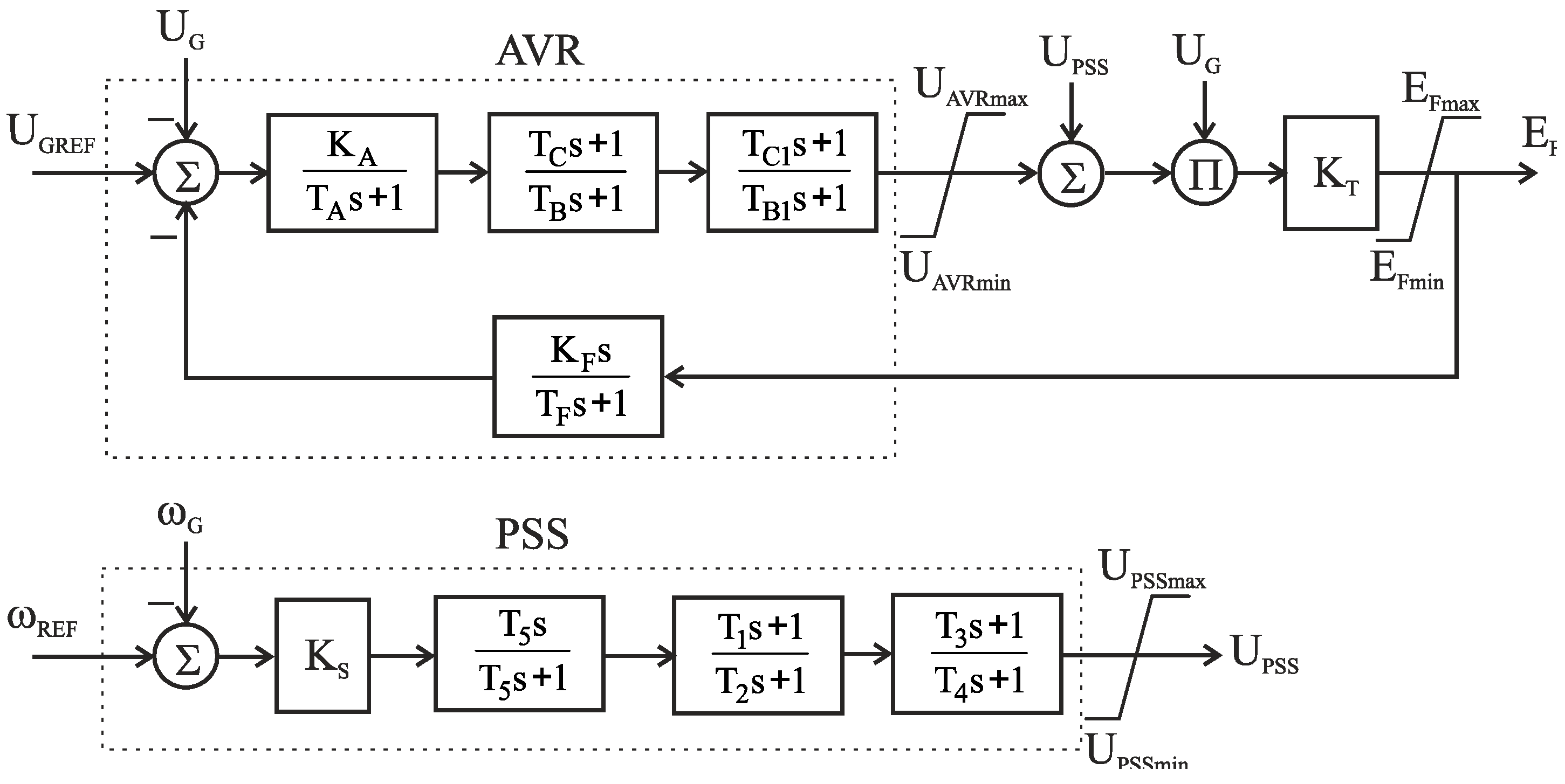
2.2. Mathematical Model of the Excitation Control System

The studied system uses a static excitation system, which is widely used for excitation control of a small and medium- power synchronous machine. In this system, the excitation voltage of the synchronous machine is regulated by a thyristor converter, the input of which is connected to the generator outputs through a step-down transformer (self-excitation circuit). Static excitation systems provide a high response of excitation control.

In the developed model, the power scheme of the excitation system is equivalent to an RL-branch with an EMF source (EXC1, EXC2), from which the value of E_F is determined by the output signal of the automatic excitation control system. In addition to the automatic excitation control system, the excitation voltage is also influenced by the generator voltage U_G, since the generator is excited according to the self-excitation scheme. A block diagram of the excitation control systems with a standard automatic voltage regulator ST1C according to [54,56] and a system stabilizer of the PSS1A type is shown in Figure 4.

All values in the block diagram are given in relative units. The system provides output signal limitations for the AVR and PSS, as well as limitations on the generator excitation voltage due to the design of the static excitation system (maximum excitation voltage in forcing mode is two nominal values).

The generator active power setpoint P_GREF is the reference signal for the turbine control system. The primary frequency control loop provides automatic power control to stabilize the frequency. The mechanical power of the turbine P_m determines the turbine torque T_t. The parameters of the turbine model block diagram are the following: D = 0.04, T_HP = 0.3 s, T_RH = 5 s, F_HP = 0.3, F_LP = 0.7.

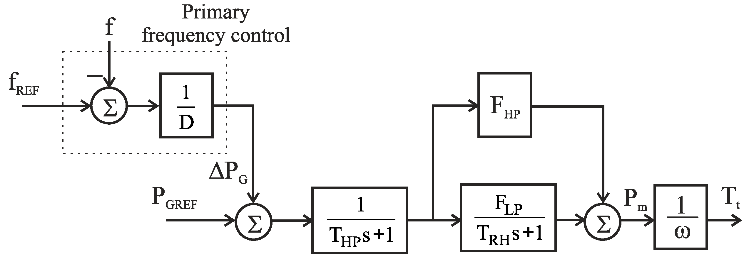
2.3. Steam Turbine Model

The structural scheme of the single reheat steam turbines with primary frequency control, according to [57,58], is shown in Figure 5.

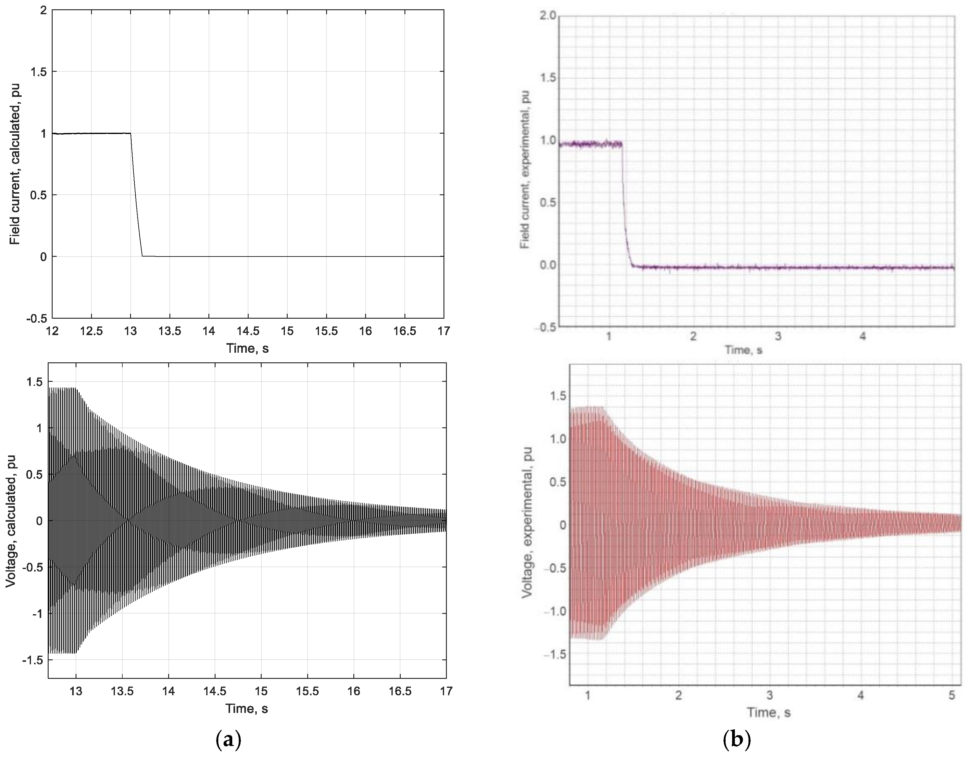
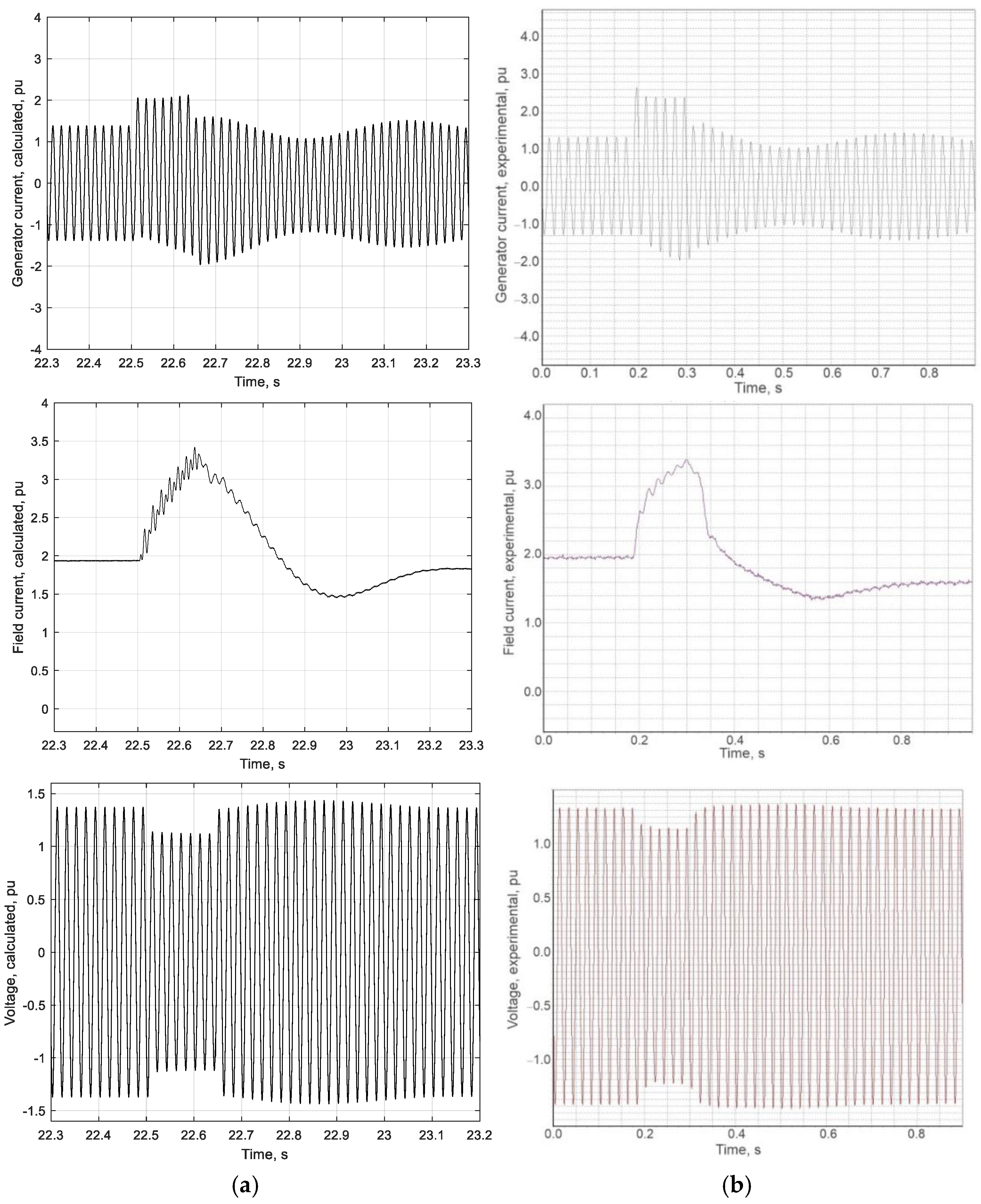
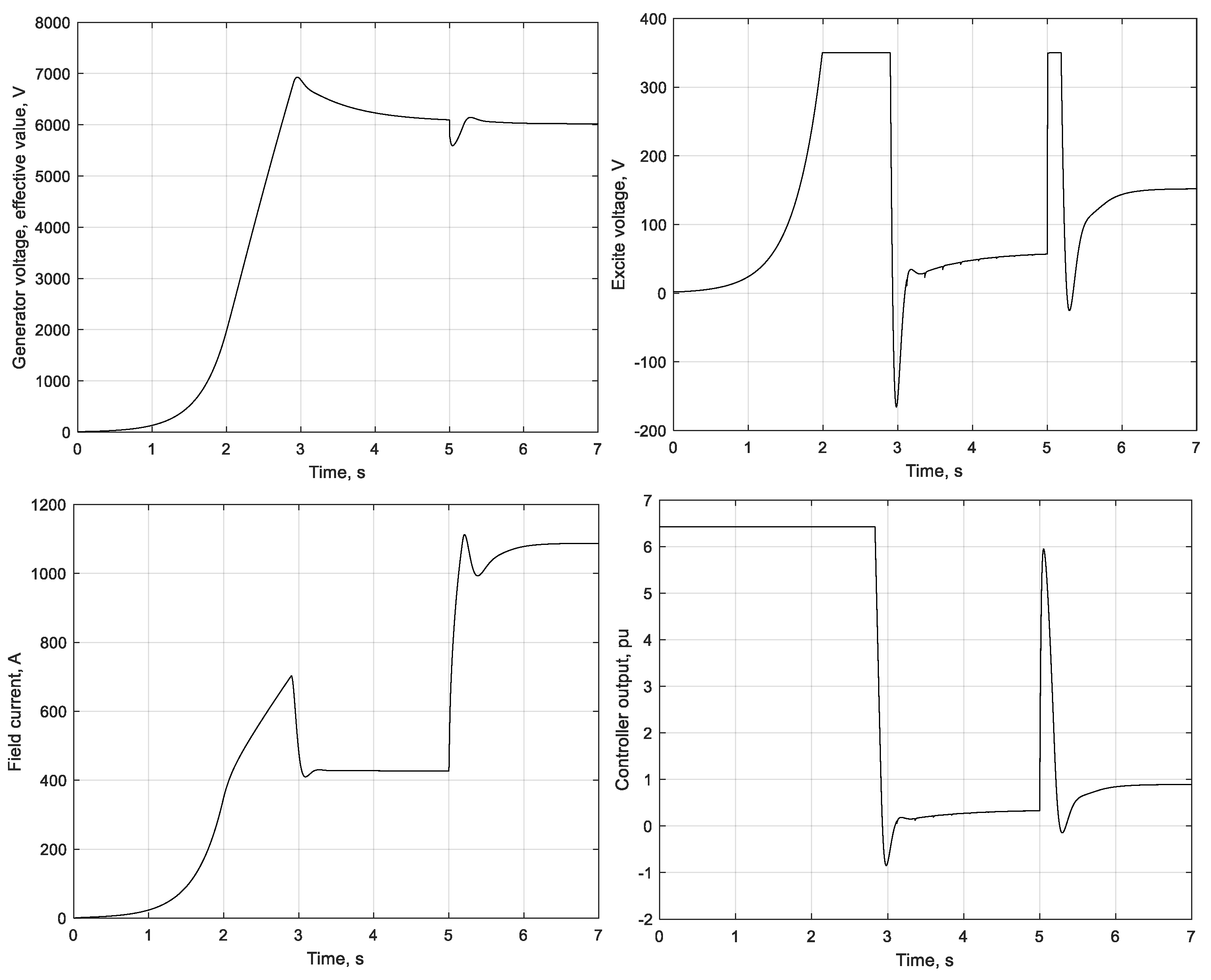
3. Verification of the Developed Mathematical Model

The developed mathematical model was verified for the system “synchronous generator with a static self-excitation system–power transformer–power grid” by comparing the experimental data obtained at Burshtyn Thermal Power Plant (Ukraine) with the results of mathematical modelling.

The generator’s parameters: the nominal power (S_n) was 235 MVA, the nominal voltage (U_n) was 15 kV, the nominal current (I_n) was 7300 A, the field current in a no-load regime (i_f) was 720 A, the stator-winding resistance was 0.00148 Ohm, and the resistance of the field winding (r_f) was 0.223 Ohm. The reactances were: X_d = 1.84 p.u., X_ad = 1.68 p.u., X_q = 1.84 p.u., X_aq = 1.68 p.u., X′_d = 0.295 p.u., X″_d = 0.19 p.u., and X″_q = 0.19 p.u. The number of pole pairs p₀ = 1. The moment of inertia (J) was 6000 kgm².

For the power transformer: the nominal power (Sn) was 250,000 kVA, the nominal voltage of the primary winding (U_1n) was 15 kV, the nominal voltage of the secondary winding (U_2n) was 347 kV, the no-load current (I₀) was 0.062 p.u., the short-circuit voltage (U_sc) was 0.11 p.u., and the active power loss was 955 kW.

For the excitation system transformer TR: the nominal power (S_n) was 2500 kVA, the nominal voltage of the primary winding (U_1n) was 15 kV, the nominal voltage of the secondary winding (U_2n) was 863 V, the no-load current (I₀) was 0.09 p.u., the short-circuit voltage (U_sc) was 0.065 p.u., and the active power loss was 22 kW. The comparison of results for the modes of initial generator excitation at no-load, de-excitation, and short circuit under the loading conditions are shown in Figure 6, Figure 7 and Figure 8.

The comparison of the modelling results and the results obtained at the real power plant demonstrates the coincidence of the character of the change in the main coordinates in different operating modes. The quantitative characteristics of the differences for the main indicators characterizing transient processes are summarized in

Table 1. Mismatch between the calculation results and experimental data on characteristic indicators.

Operation Mode	Characteristic Indicators	Mismatch Value, %
Initial generator excitation at no-load	Amplitude of excitation current oscillations at the beginning of the transient process	4
	Duration of initial excitation	2.5
	Overshoot of excitation current	2
	Generator voltage steady-state value	1.2
De-excitation of the generator	Time for the excitation current to drop off	4.8
	Time for the generator voltage to drop to 10% of the nominal value, Tde	5
	Generator voltage decrease in time 0.5Tde	2
Short-circuit in power line	The effective stator current value during short-circuit	14
	Maximum stator current instantaneous value after short-circuit disconnection	11
	Minimum amplitude value of the stator current after short-circuit disconnection	2
	Period of self-oscillation after short-circuit disconnection	5.5
	The maximum value of the excitation current	6
	The minimum value of the excitation current (after short-circuit disconnection)	8
	Generator voltage during short-circuit	3
	Maximum generator voltage instantaneous value after short-circuit disconnection	7
	Average value	4.3

.

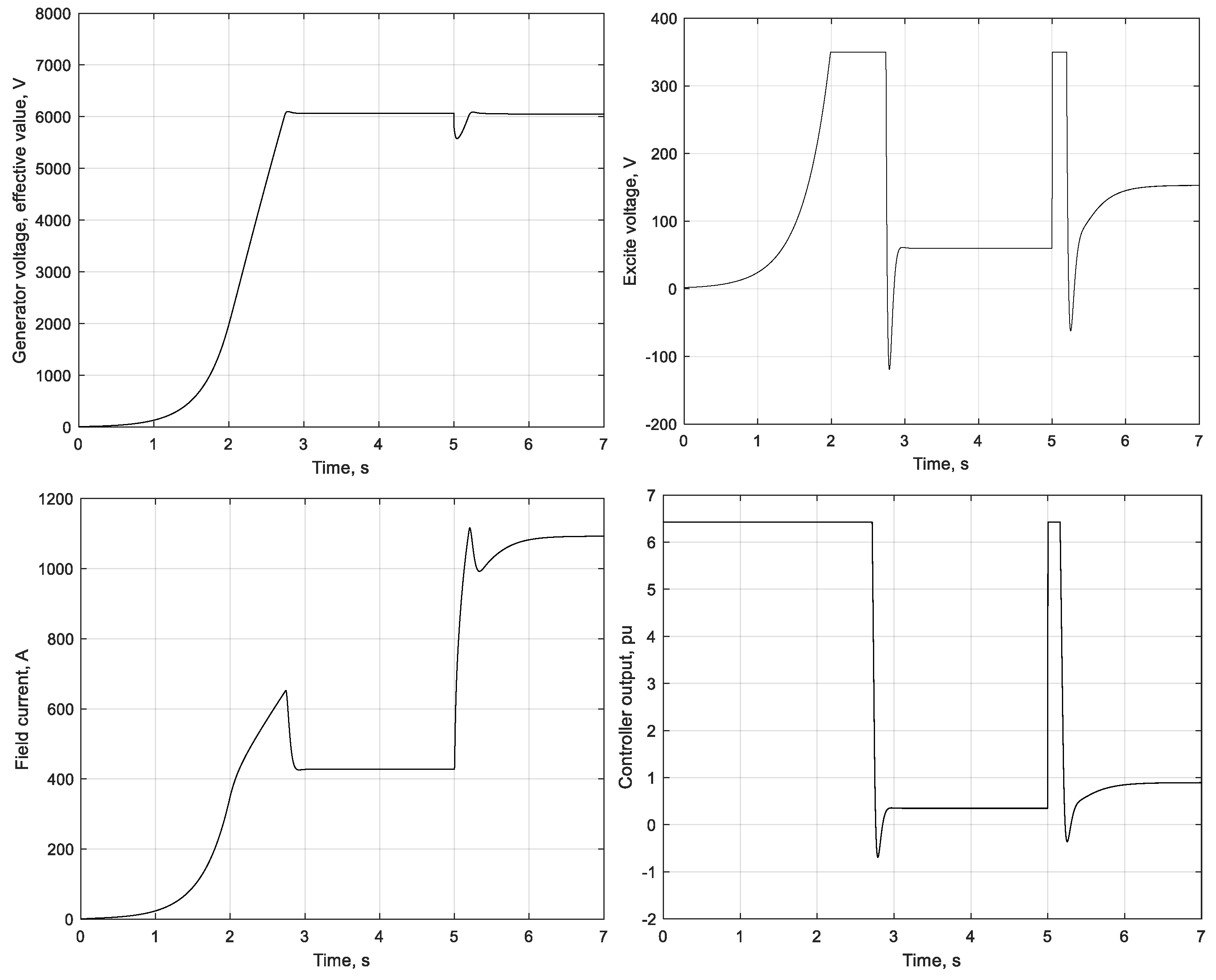
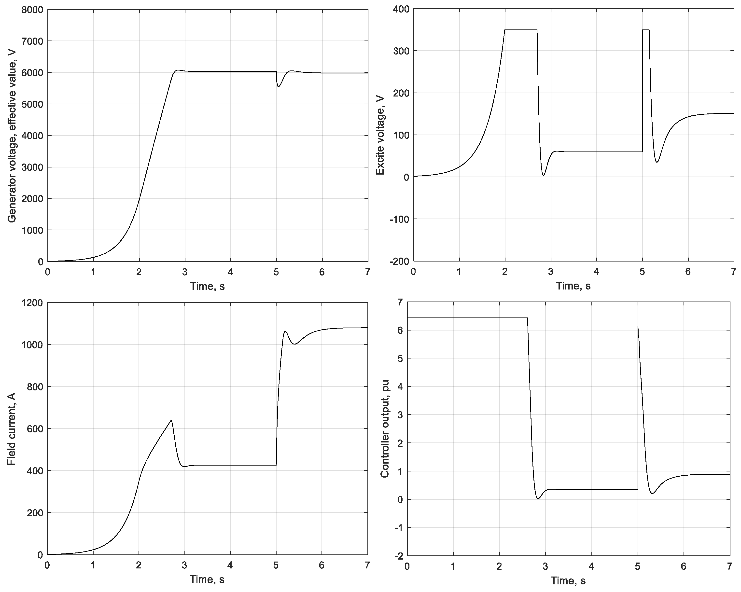
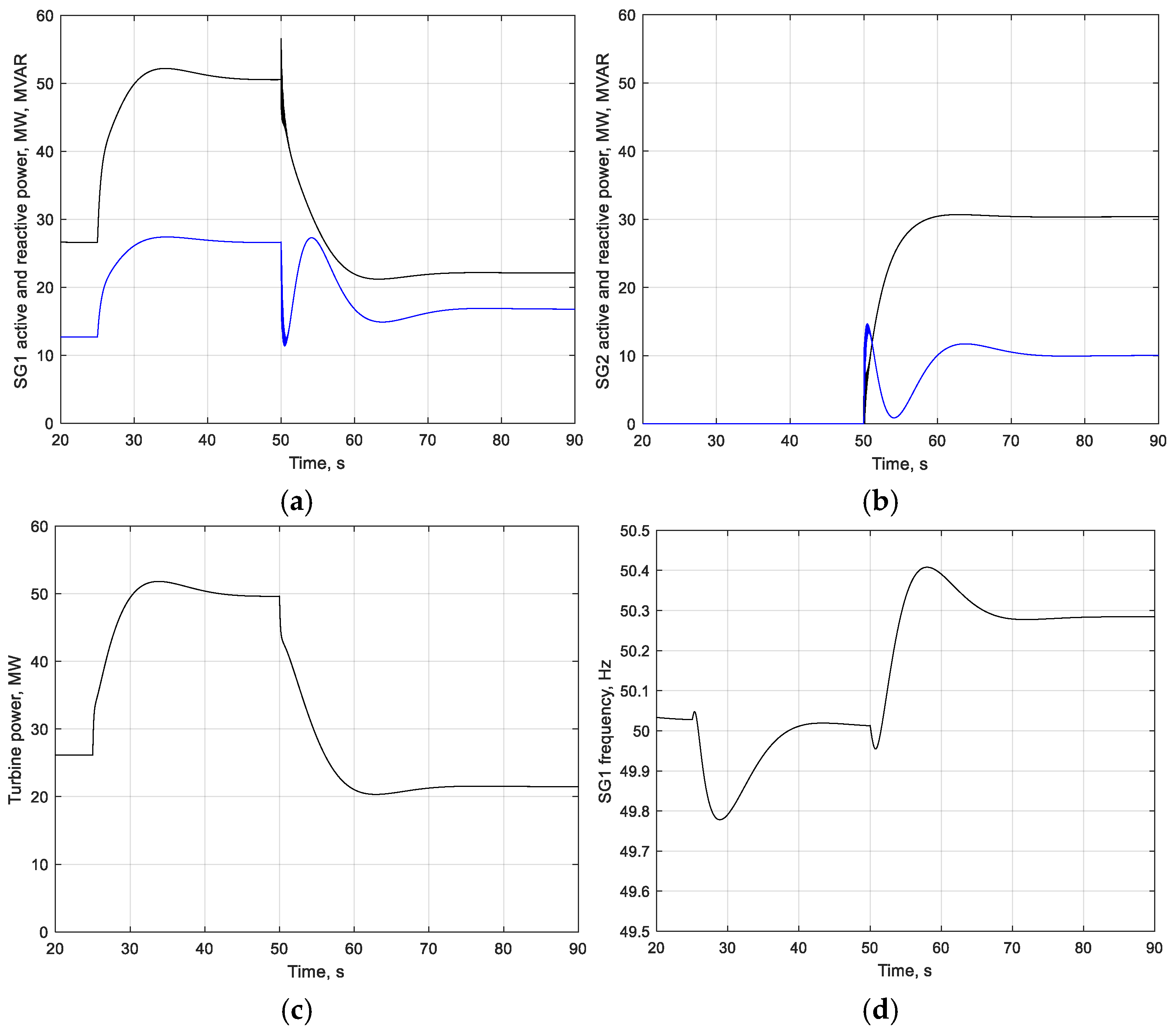
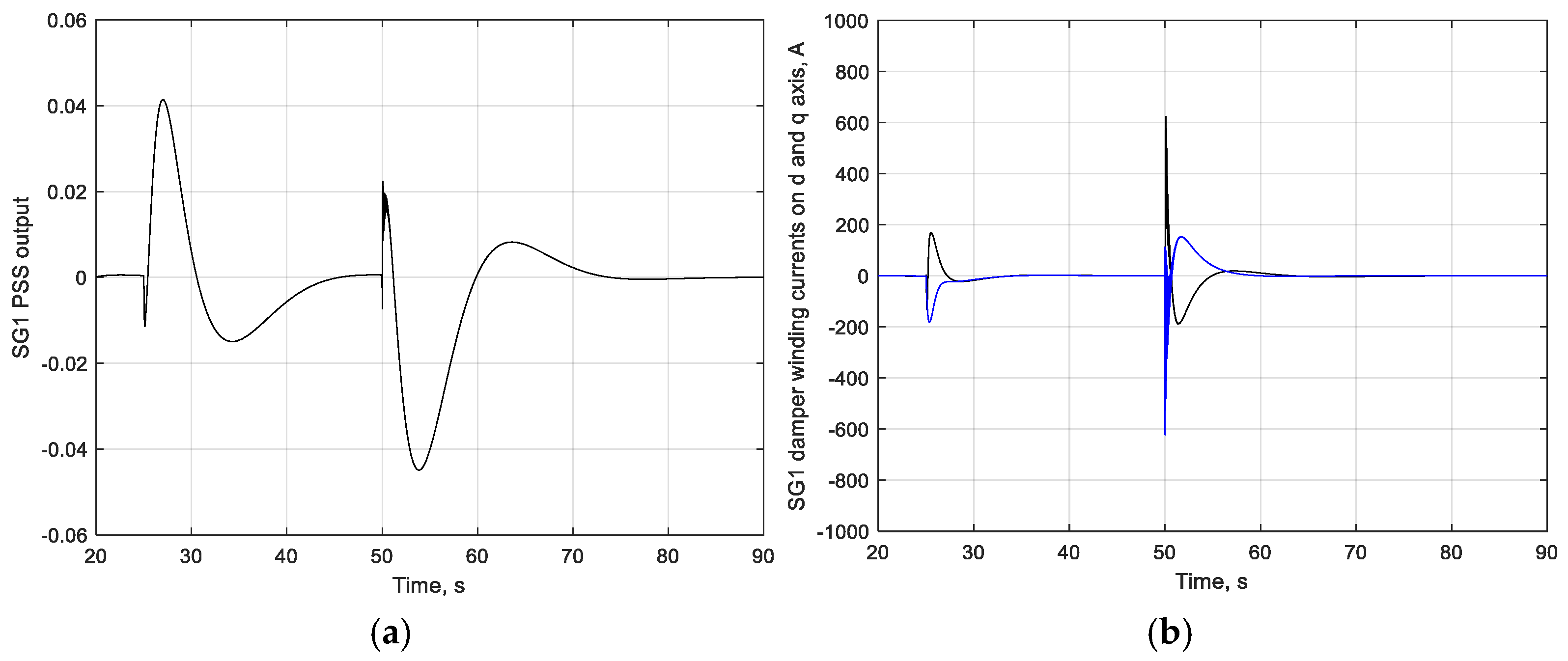
4. Simulation Results

The results for the system with the synthesized fractional order voltage controller in comparison with the known voltage control systems for the modes of initial generator excitation at no-load and abrupt rated loading are shown in Figure 9, Figure 10 and Figure 11.

The generator’s parameters, which are used in this research are the following: the nominal power (S_n) 63 MVA, the nominal voltage 10.5 kV, the nominal current 4300 A, the nominal field current 1230 A, the nominal excite voltage 172 V. The reactances were: X_d = 2.11 p.u., X_ad = 2.2 p.u., X_q = 2.2 p.u., X_aq = 2.11 p.u., X′_d = 0.224 p.u., X″_d = 0.139 p.u. The number of pole pairs p₀ = 1.

Parameters of AVR are the following. For AVR with rate feedback on generator excitation voltage [54]: K_A = 110, T_A = 0.02 s, T_C = T_B = T_C1 = T_B1 = 0, K_F = 0.005, T_F = 0.7 s. For AVR with P-voltage controller and lead–lag block in the forward path [54]: K_A = 190, T_A = 0 s, T_C = 1 s, T_B = 1 s, T_C1 = T_B1 = 0, K_F = 0, T_F = 0 s.

The results presented in Figure 9 show that the implementation of rate feedback on the generator excitation voltage affects the quality of the transient process of the initial generator excitation in a self-excited system, since such feedback slows down the voltage control performance (while increasing the damping of the excitation current in transient modes). This leads to the occurrence of overregulation in a self-excited system (this effect is absent for systems with independent excitation).

The proposed fractional-order controller provides a better quality of transients, similar to those obtained in the system with a P-voltage controller and lead–lag block in the forward path. However, the advantage of using the fractional-order controller is the much smaller oscillations in the intermediate coordinates, in particular, the generator excitation voltage (Figure 10 and Figure 11). In addition, the same quality of transients is ensured at lower values of the voltage gain (50 for the AVR with fractional-order controller, 190 for the AVR with P-voltage controller and lead–lag block in the forward path).

The results presented in Figure 12, Figure 13, Figure 14 and Figure 15 demonstrate the operation of a synchronous generator in a two-bus system (Figure 3) with the proposed voltage control system in load-varying modes, taking into account the influence of the system stabilizer as part of the excitation control system, the turbine control system (Figure 5) and the influence of the parallel-operating SM2 generator.

The studies were carried out for the case of load increase for SM1 with an active power of up to 50 MW and a reactive power of up to 27 MVA (at a time point of 25 s, Figure 12), followed by parallel connection of the SM2 generator at a time point of 50 sec with the latter simultaneous loading SM2 with a capacity of 30 MW at a constant load in the system. After the SM2 generator was switched on, the power assignment of the SM1 turbine was reduced by 20 MW. At the same time, due to the primary frequency control as part of the turbine control system, the real power of the turbine decreased by 28 MW (Figure 12c).

The PSS system stabilizer, as part of the excitation control system, affects the excitation current to dampen the SM1 speed (frequency) fluctuations (Figure 13a). Such changes in speed can be caused by changes in the power generated by parallel generators, as well as frequency fluctuations in the grid due to changes in energy consumption [58]. Analyzing the influence of the structure and parameters of the PSS on the damping of frequency fluctuations in the power grid is an important task that is beyond the scope of this research. Figure 13b shows the calculated currents of the damping winding of SM1 along the d and q axes, which also dampen the oscillations of the generator.

As the study results show, the proposed generator voltage control system with a fractional-order controller provides sufficiently high quality generator voltage stabilization in the specified modes with a dynamic error of up to 4.5% (Figure 14b), which is a good indicator.

It should be noted that the developed model operates in phase coordinates, which in further studies will make it possible to analyze asymmetric modes, in particular, short circuits. Figure 15 illustrates the instantaneous values of the phase currents of the stator windings SM1 and SM2 in the above modes.

5. Conclusions

The proposed system of automatic generator voltage control with a fractional-order controller provides high quality transients similar to the system with a P-voltage controller with a lead–lag block in the forward path with a standard configuration. However, the advantage of using a fractional-order controller is the significantly lower oscillations in the intermediate coordinates, in particular the generator excitation voltage. In addition, the same quality of transients is ensured at lower values of the voltage gain (50 for the AVR with fractional-order controller, 190 for the AVR with P-voltage controller and lead–lag block in the forward path), which provides a greater system-stability margin. According to the research results, taking into account the influence of a parallel generator and the mutual influence of the main control loops (turbine and system stabilizer), the proposed system provides a dynamic voltage control error in the modes of generator load change of up to 4.5%, which is a good result. The research results demonstrate the importance of a comprehensive consideration of the interaction of various generator control systems (AVR, PSS and turbine control) to analyze generator operation under the influence of various disturbances in the power system and to improve the stabilization of the frequency and voltage in the electrical grid.

References

1. Buongiorno, J.; Corradini, M.; Parsons, J.; Petti, D. Nuclear Energy in a Carbon-Constrained World: Big Challenges and Big Opportunities. IEEE Power Energy Mag. 2019, 17, 69–77. [Google Scholar] [CrossRef]
2. Lloyd, C.A.; Roulstone, T.; Lyons, R.E. Transport, constructability, and economic advantages of SMR modularization. Prog. Nucl. Energy 2021, 134, 103672. [Google Scholar] [CrossRef]
3. Poudel, B.; Gokaraju, R. Small Modular Reactor (SMR) Based Hybrid Energy System for Electricity & District Heating. IEEE Trans. Energy Convers. 2021, 36, 2794–2802. [Google Scholar] [CrossRef]
4. Poudel, B.; Joshi, K.; Gokaraju, R. A Dynamic Model of Small Modular Reactor Based Nuclear Plant for Power System Studies. IEEE Trans. Energy Convers. 2020, 35, 977–985. [Google Scholar] [CrossRef]
5. Jenkins, J.D.; Zhou, Z.; Ponciroli, R.; Vilim, R.B.; Ganda, F.; de Sisternes, F.; Botterud, A. The benefits of nuclear flexibility in power system operations with renewable energy. Appl. Energy 2018, 222, 872–884. [Google Scholar] [CrossRef]
6. Wang, Y.; Chen, W.; Zhang, L.; Zhao, X.; Gao, Y.; Dinavahi, V. Small Modular Reactors: An Overview of Modeling, Control, Simulation, and Applications. IEEE Access 2024, 12, 39628–39650. [Google Scholar] [CrossRef]
7. Anderson, P.M.; Fouad, A.A. Power System Control and Stability; IEEE Press: Piscataway, NJ, USA, 1994. [Google Scholar]
8. Law, K.T.; Hill, D.J.; Godfrey, N.R. Robust controller structure for coordinated power system voltage regulator and stabilizer design. IEEE Trans. Control Syst. Technol. 1994, 2, 220–232. [Google Scholar] [CrossRef]
9. Kundur, P. Power Systems Stability and Control; McGraw-Hill, Inc.: New York, NY, USA, 1994. [Google Scholar]
10. Mira-Gebauer, N.; Rahmann, C.; Álvarez-Malebrán, R.; Vittal, V. Review of Wide-Area Controllers for Supporting Power System Stability. IEEE Access 2023, 11, 8073–8095. [Google Scholar] [CrossRef]
11. Verrelli, C.M.; Marino, R.; Tomei, P.; Damm, G. Nonlinear Robust Coordinated PSS-AVR Control for a Synchronous Generator Connected to an Infinite Bus. IEEE Trans. Autom. Control 2022, 67, 1414–1422. [Google Scholar] [CrossRef]
12. Machowski, J.; Robak, S.; Bialek, J.W.; Bumby, J.R.; Abi-Samra, N. Decentralized stability-enhancing control of synchronous generator. IEEE Trans. Power Syst. 2000, 15, 1336–1344. [Google Scholar] [CrossRef]
13. Cao, Y.; Jiang, L.; Cheng, S.; Chen, D.; Malik, O.P.; Hope, G.S. A nonlinear variable structure stabilizer for power system stability. IEEE Trans. Energy Convers. 1994, 9, 489–495. [Google Scholar] [CrossRef]
14. Loukianov, A.G.; Cañedo, J.M.; Fridman, L.M.; Soto-Cota, A. High-Order Block Sliding-Mode Controller for a Synchronous Generator With an Exciter System. IEEE Trans. Ind. Electron. 2011, 58, 337–347. [Google Scholar] [CrossRef]
15. Doria-Cerezo, A.; Utkin, V.I.; Munoz-Aguilar, R.S.; Fossas, E. Control of a Stand-Alone Wound Rotor Synchronous Generator: Two Sliding Mode Approaches via Regulation of the d-Voltage Component. IEEE Trans. Control Syst. Technol. 2012, 20, 779–786. [Google Scholar] [CrossRef]
16. Liu, X.; Han, Y. Decentralized multi-machine power system excitation control using continuous higher-order sliding mode technique. Int. J. Electr. Power Energy Syst. 2016, 82, 76–86. [Google Scholar] [CrossRef]
17. Li, J.; Liu, Y.; Li, C.; Chu, B. Passivity-Based Nonlinear Excitation Control of Power Systems with Structure Matrix Reassignment. Information 2013, 4, 342–350. [Google Scholar] [CrossRef]
18. Biletskyi, Y.O.; Shchur, I.Z.; Kuzyk, R.-I.V. Passivity-based control system for stand-alonehybrid electrogenerating complex. Appl. Asp. Inf. Technol. 2021, 4, 140–152. [Google Scholar] [CrossRef]
19. Dong, Z.; Cheng, Z.; Lin, X.; Zhu, Y.; Chen, F.; Huang, X. Passivity-Based Control of Nuclear Reactors Considering Cold Side Temperature. In Proceedings of the IECON 2023—49th Annual Conference of the IEEE Industrial Electronics Society, Singapore, 16–19 October 2023; pp. 1–6. [Google Scholar] [CrossRef]
20. Roy, T.K.; Mahmud, M.A.; Shen, W.; Oo, A.M.T.; Haque, M.E. Robust nonlinear adaptive backstepping excitation controller design for rejecting external disturbances in multimachine power systems. Int. J. Electr. Power Energy Syst. 2017, 84, 76–86. [Google Scholar] [CrossRef]
21. Roy, T.K.; Mahmud, M.A.; Shen, W.; Oo, A.M.T. Nonlinear Adaptive Excitation Controller Design for Multimachine Power Systems With Unknown Stability Sensitive Parameters. IEEE Trans. Control Syst. Technol. 2017, 25, 2060–2072. [Google Scholar] [CrossRef]
22. Liying, S.; Zhihua, L. Nonlinear adaptive backstepping control for synchronous generator excitation system with output constraints. In Proceedings of the Fifth International Conference on Intelligent Control and Information Processing, Dalian, China, 18–20 August 2014; pp. 336–340. [Google Scholar] [CrossRef]
23. Long, B.; Liao, Y.; Chong, K.T.; Rodríguez, J.; Guerrero, J.M. MPC-Controlled Virtual Synchronous Generator to Enhance Frequency and Voltage Dynamic Performance in Islanded Microgrids. IEEE Trans. Smart Grid 2021, 12, 953–964. [Google Scholar] [CrossRef]
24. Kiaei, I.; Rostami, M.; Lotfifard, S. Robust Decentralized Control of Synchronous Generators for Improving Transient Stability of Multimachine Power Grids. IEEE Syst. J. 2021, 15, 3470–3479. [Google Scholar] [CrossRef]
25. Zheng, Y.; Zhou, J.; Zhu, W.; Zhang, C.; Li, C.; Fu, W. Design of a multi-mode intelligent model predictive control strategy for hydroelectric generating uni. Neurocomputing 2016, 207, 287–299. [Google Scholar] [CrossRef]
26. Orchi, T.F.; Roy, T.K.; Mahmud, M.A.; Oo, A.M.T. Feedback Linearizing Model Predictive Excitation Controller Design for Multimachine Power Systems. IEEE Access 2018, 6, 2310–2319. [Google Scholar] [CrossRef]
27. Kenné, G.; Goma, R.; Nkwawo, H.; Lamnabhi-Lagarrigue, F.; Arzandé, A.; Vannier, J.C. An improved direct feedback linearization technique for transient stability enhancement and voltage regulation of power generators. Int. J. Electr. Power Energy Syst. 2010, 32, 809–816. [Google Scholar] [CrossRef]
28. Roy, T.K.; Mahmud, M.A.; Shen, W.X.; Oo, A.M.T. An Adaptive Partial Feedback Linearizing Control Scheme: An Application to a Single Machine Infinite Bus System. IEEE Trans. Circuits Syst. II Express Briefs 2020, 67, 2557–2561. [Google Scholar] [CrossRef]
29. Leon, A.E.; Solsona, J.A.; Valla, M.I. Comparison among nonlinear excitation control strategies used for damping power system oscillations. Energy Convers. Manag. 2012, 53, 55–67. [Google Scholar] [CrossRef]
30. Mahmud, M.A.; Pota, H.R.; Aldeen, M.; Hossain, M.J. Partial Feedback Linearizing Excitation Controller for Multimachine Power Systems to Improve Transient Stability. IEEE Trans. Power Syst. 2014, 29, 561–571. [Google Scholar] [CrossRef]
31. Rigatos, G.; Siano, P.; Melkikh, A.; Zervos, N. A Nonlinear H-Infinity Control Approach to Stabilization of Distributed Synchronous Generators. IEEE Syst. J. 2018, 12, 2654–2663. [Google Scholar] [CrossRef]
32. Ugalde-Loo, C.E.; Acha, E.; Licéaga-Castro, E. Multi-machine power system state-space modelling for small-signal stability assessments. Appl. Math. Model. 2013, 37, 10141–10161. [Google Scholar] [CrossRef]
33. Fathollahi, A.; Andresen, B. Multi-Machine Power System Transient Stability Enhancement Utilizing a Fractional Order-Based Nonlinear Stabilizer. Fractal Fract. 2023, 7, 808. [Google Scholar] [CrossRef]
34. Ugalde Loo, C.E.; Vanfretti, L.; Liceaga-Castro, E.; Acha, E. Synchronous Generators Modeling and Control Using the Framework of Individual Channel Analysis and Design: Part 1. Int. J. Emerg. Electr. Power Syst. 2007, 5, 1–25. [Google Scholar] [CrossRef]
35. Wang, X.; Chen, Y.; Han, G.; Song, C. Nonlinear dynamic analysis of a single-machine infinite-bus power system. Appl. Math. Model. 2015, 39, 2951–2961. [Google Scholar] [CrossRef]
36. Panday, R.; Harun, N.F.; Zhang, B.; Maloney, D.; Tucker, D.; Bayham, S. Analyzing Gas Turbine-Generator Performance of the Hybrid Power System. IEEE Trans. Power Syst. 2022, 37, 543–550. [Google Scholar] [CrossRef]
37. Badakhshan, S.; Senemmar, S.; Zhang, J. Dynamic Modeling and Reliable Operation of All-Electric Ships with Small Modular Reactors and Battery Energy Systems. In Proceedings of the 2023 IEEE Electric Ship Technologies Symposium (ESTS), Alexandria, VA, USA, 1–4 August 2023; pp. 327–332. [Google Scholar] [CrossRef]
38. Wang, L.; Zeng, S.-Y.; Feng, W.-K.; Prokhorov, A.V.; Mokhlis, H.; Huat, C.K. Damping of Subsynchronous Resonance in a Hybrid System With a Steam-Turbine Generator and an Offshore Wind Farm Using a Unified Power-Flow Controller. IEEE Trans. Ind. Appl. 2021, 57, 110–120. [Google Scholar] [CrossRef]
39. Ouassaida, M.; Maaroufia, M.; Cherkaoui, M. A real-time nonlinear decentralized control of multimachine power systems. Syst. Sci. Control. Eng. Open Access J. 2014, 2, 135–142. [Google Scholar] [CrossRef]
40. Kutsyk, A.; Semeniuk, M.; Korkosz, M.; Podskarbi, G. Diagnosis of the Static Excitation Systems of Synchronous Generators with the Use of Hardware-In-the-Loop Technologies. Energies 2021, 14, 6937. [Google Scholar] [CrossRef]
41. Sabir, A.; Michaelson, D.; Jiang, J. Load-Frequency Control With Multimodule Small Modular Reactor Configuration: Modeling and Dynamic Analysis. IEEE Trans. Nucl. Sci. 2021, 68, 1367–1380. [Google Scholar] [CrossRef]
42. Zhang, Q.-H.; Lu, J.-G.; Xu, J.; Chen, Y.-Q. Solution Analysis and Novel Admissibility Conditions of SFOSs: The 1 < α < 2 Case. IEEE Trans. Syst. Man Cybern. Syst. 2022, 52, 5056–5067. [Google Scholar] [CrossRef]
43. Yu, Y.; Guan, Y.; Kang, W.; Chaudhary, S.K.; Vasquez, J.C.; Guerrero, J.M. Fractional-Order Virtual Synchronous Generator. IEEE Trans. Power Electron. 2023, 38, 6874–6879. [Google Scholar] [CrossRef]
44. Gulzar, M.M.; Gardezi, S.; Sibtain, D.; Khalid, M. Discrete-Time Modeling and Control for LFC Based on Fuzzy Tuned Fractional-Order PDμ Controller in a Sustainable Hybrid Power System. IEEE Access 2023, 11, 63271–63287. [Google Scholar] [CrossRef]
45. AbdelAty, A.M.; Al-Durra, A.; Zeineldin, H.H.; Kanukollu, S.; El-Saadany, E.F. Enhancing Dynamic Performance of Islanded Microgrids by Fractional-Order Derivative Droop. IEEE Trans. Ind. Inform. 2024, 20, 9427–9444. [Google Scholar] [CrossRef]
46. Kazemi, M.V.; Sadati, S.J.; Gholamian, S.A. Adaptive Frequency Control of Microgrid Based on Fractional Order Control and a Data-Driven Control With Stability Analysis. IEEE Trans. Smart Grid 2022, 13, 381–392. [Google Scholar] [CrossRef]
47. Podlubny, I. Fractional-order systems and PIλDμ-controllers. IEEE Trans. Autom. Control 1999, 44, 208–214. [Google Scholar] [CrossRef]
48. Pan, I.; Das, S. Chaotic multi-objective optimization based design of fractional order PIλDμ controller in AVR system. Int. J. Electr. Power Energy Syst. 2012, 43, 393–407. [Google Scholar] [CrossRef]
49. Xue, D.; Zhao, C.; Chen, Y. A Modified Approximation Method of Fractional Order System. In Proceedings of the 2006 International Conference on Mechatronics and Automation, Luoyang, China, 25–28 June 2006; pp. 1043–1048. [Google Scholar] [CrossRef]
50. Birs, I.; Muresan, C.; Nascu, I.; Ionescu, C. A Survey of Recent Advances in Fractional Order Control for Time Delay Systems. IEEE Access 2019, 7, 30951–30965. [Google Scholar] [CrossRef]
51. Caputo, M.; Fabrizio, M. A New Definition of Fractional Derivative without Singular Kernel. Prog. Fract. Differ. Appl. 2015, 2, 73–85. [Google Scholar]
52. Losada, J.; Nieto, J.J. Properties of a new fractional derivative without singular kernel. Prog. Fract. Differ. Appl. 2016, 1, 87–92. [Google Scholar]
53. Nchama, G.A.M.; Mecıas, A.L.; Richard, M.R. The Caputo-Fabrizio Fractional Integral to Generate Some New Inequalities. Inf. Sci. Lett. 2019, 8, 73–80. [Google Scholar]
54. IEEE Std 421.5-2016; IEEE Recommended Practice for Excitation System Models for Power System Stability Studies—Redline. IEEE: New York, NY, USA, 2016; pp. 1–453.
55. Plakhtyna, O.; Kutsyk, A.; Lozynskyy, A. Method of average voltages in integration step: Theory and application. Electr. Eng. 2020, 102, 2413–2422. [Google Scholar] [CrossRef]
56. Boudot, C.; Droin, J.-B.; Sciora, P.; Besanger, Y.; Robisson, B.; Mazauric, A.-L. Small Modular Reactor-based solutions to enhance grid reliability: Impact of modularization of large power plants on frequency stability. EPJ N—Nucl. Sci. Technol. 2022, 8, 16. [Google Scholar] [CrossRef]
57. Göran, A. Dynamics and Control of Electric Power Systems; EEH—Power Systems Laboratory; ETH Zurich: Zurich, Switzerland, 2012. [Google Scholar]
58. Avon, G.; Bucolo, M.; Buscarino, A.; Fortuna, L. Sensing Frequency Drifts: A Lookup Table Approach. IEEE Access 2022, 10, 96249–96259. [Google Scholar] [CrossRef]
Figure 1. Functional scheme of the examined system.
Energies 17 05913 g001
Figure 2. Calculation scheme of the synchronous machine.
Energies 17 05913 g002
Figure 3. Calculation scheme of the power system.
Energies 17 05913 g003
Figure 4. Structural scheme of exciter controller.
Energies 17 05913 g004
Figure 5. Structural scheme of steam turbine model.
Energies 17 05913 g005
Figure 6. Simulation (a), experimental (b) results of the field current (if) and terminal voltage of the generator (ug, instantaneous value) for the initial excitation of the generator.
Energies 17 05913 g006
Figure 7. Simulation (a), experimental (b) results of the field current (if) and terminal voltage of the generator (ug, instantaneous value) for the de-excitation of the generator.
Energies 17 05913 g007
Figure 8. Simulation (a), experimental (b) results of the stator current (ig), field current (if), and terminal voltage of the generator (ug, instantaneous value) for short-circuit in power line.
Energies 17 05913 g008
Figure 9. Simulation results for initial excitation in the system with rate feedback on generator excitation voltage.
Energies 17 05913 g009
Figure 10. Simulation results for initial excitation in the system with P-voltage controller and lead–lag block in the forward path.
Energies 17 05913 g010
Figure 11. Simulation results for initial excitation in the system with proposed fractional-order controller.
Energies 17 05913 g011
Figure 12. Simulation results for two-machine system under loading variations: active (black) and reactive (blue)-SM1 (a), active (black) and reactive (blue)-SM2 (b), SM1′s turbine power (c) and frequency at output of SM1 (d).
Energies 17 05913 g012
Figure 13. Simulation results for two-machine system under loading variation: SM1′s PSS output (a), SM1’s damper winding current on d- (black) and q- (blue) axis (b).
Energies 17 05913 g013
Figure 14. Simulation results for two-machine system under loading variations: field current of SM1 (a), effective value of SM1′s stator phase voltage (b).
Energies 17 05913 g014
Figure 15. Simulation results for two-machine system under loading variations: instantaneous value of stator phase current of SM1 (a) and SM2 (b).
Energies 17 05913 g015