Panel Temperature Dependence on Atmospheric Parameters of an Operative Photovoltaic Park in Semi-Arid Zones Using Artificial Neural Networks

Abstract

The performance of photovoltaic solar panels is influenced by their temperature, so there is a need for a tool that can accurately and instantly predict the panel temperature. This paper presents an analysis of the panel temperature’s dependence on atmospheric parameters at an operational photovoltaic park in the semi-arid north of Chile using Artificial Neural Networks (ANNs). We applied the back-propagation algorithm to train the model by using the atmospheric variables tilted solar radiation (TSR), air temperature, and wind speed measured in the park. The ANN model’s effectiveness was evaluated by comparing it to five different deterministic models: the Standard model, King’s model, Faiman’s model, Mattei’s model, and Skoplaki’s model. Additionally, we examined the sensitivity of panel temperature to changes in air temperature, TSR, and wind speed. Our findings show that the ANN model had the best prediction accuracy for panel temperature, with a Root Mean Squared Error (RMSE) of 1.59 °C, followed by Mattei’s model with a higher RMSE of 3.30 °C. We also determined that air temperature has the most significant impact on panel temperature, followed by TSR and wind speed. These results demonstrate that the ANN is a powerful tool for predicting panel temperature with high accuracy.

1. Introduction

The continued use of fossil fuels has led to an accelerated increase in greenhouse gas concentration such as CO₂, which is recognized as one of the main causes of global warming. To protect the planet from this effect, researchers are continuously looking towards alternative renewable energy sources (RESs) [1]. In this context, several countries have developed policies to incentivize the insertion of RESs in their electricity matrix. A good example is Chile’s case, where the installed power of RESs at the end of 2021 was 16.9 GW, which corresponds to 54.8% of the total electric capacity, aiming to grow to 70% by 2050. From the total RESs installed, 39.1% corresponds to photovoltaic (PV) parks [2].

The north of Chile is known as one of the places with the highest solar radiation worldwide. The Atacama Desert presents an annual global radiation of 2.6 MWh m⁻² [3], which shows its great potential for PV solar energy development.

Despite high solar radiation, the power generation of the panels is affected by a variety of effects, such as soiling [4] and high temperatures [5,6]. PV solar cells are designed to operate at optimal conditions when the cell temperature is 25 °C; however, under field conditions, modules—and thus the cells—can easily exceed 40 °C [5] and can go as high as 80 °C in extreme arid zones [7], leading to a reduction in power conversion efficiency (PCE) [5,8,9]. The decrease in the PCE is a consequence of a drop in the open circuit voltage (VOC) of the solar cell as the module temperature increases. It has been reported that the PCE decreases between 0.25% and 0.50% every °C [8,10]. The decrease in the PCE by increasing panel temperature has a high significant economic impact, especially in large PV arrays. Therefore, having a model that allows us to predict the panel temperature accurately can help to mitigate economic losses.

Several authors have proposed analytical deterministic models to predict the PV cell temperature from atmospheric parameters, such as solar radiation, air temperature, and wind speed [8,11,12,13,14,15]. O. Ayvazoğluyüksel, 2018, used these models to predict PV panel temperature for solar power forecasting [16]. C. Schwingshackl, 2013, compared deterministic models for different PV technologies [17]. The authors showed that there is good agreement between the models and the observations, with Mattei’s model the one with the best fit. However, in the case of polycrystalline cells, the authors found that Mattei’s model presented an error of nearly 3 °C, which could lead to a reduction in PCE of up to 1.5%. Accordingly, there is still a need to reduce the error in panel temperature predictions.

Recently, ref. [18] developed a dynamic model to predict panel temperature. The model is based on energy balance equations, considering atmospheric parameters and heat transfer processes inside the modules, as well as between modules and their environment. The proposed model showed a high predictive capacity, accuracy and robustness. However, it required a large number of input variables and coefficients, which are not always available, especially when an operative power plant is under study. This makes the model difficult to implement.

Another way to predict the PV cell temperature from atmospheric variables is by using machine learning methods (MLMs). According to [19], MLM works without any prior knowledge of the system’s characteristics, giving insights into the dependencies between the variables of a dataset. There are different MLMs available to simulate complex non-linear problems, such as Random Forest (RF), Support Vector Machines (SVMs), and Artificial Neural Networks (ANNs) [19,20]. Ref. [9] simulated the panel temperature from atmospheric and operating variables of a PV system using different MLMs—SVMs, Regression Tree ensembles, and two different ANN algorithms. The authors found that, among these methods, the ANNs showed the best performance.

Several authors describe ANNs as a system that imitates the human brain to solve linear and non-linear problems [21]. ANNs have been widely used to predict a wide range of processes, such as arsenic removal [22] and power generation by a wind turbine [23,24]. Similarly, ANNs have been used for different issues related to solar energy applications, such as solar power generation forecasting [25,26] and solar irradiation forecasting [27].

Some authors have reported the usage of an ANN to predict the temperature of photovoltaic cells. Ref. [28] applied a back-propagation algorithm to predict panel temperature, taking in account air temperature and solar radiation; ref. [29] used an ANN to predict panel temperature as a function of weather and electrical parameters; ref. [30] developed an ANN model to estimate panel temperature considering operation parameters; ref. [31] predicted the panel temperature of a high-concentrator PV (HCPV) system from atmospheric and operational parameters, using different approaches, including an ANN; and ref. [32] used an ANN and analytical models to predict panel temperature, implicating atmospheric parameters in Bangalore, India. The model was based on data recorded every second for a period of 12 days; ref. [9] used an ANN and other AI methods to predict panel temperature from atmospheric variables, taking three years of data.

However, all these works were carried out in small PV systems (up to ~kWp) and under total or partially controlled conditions.

This paper aims to predict the panel temperature of an operative PV power plant located in the semi-arid Coquimbo Region in Chile using an ANN and to compare the results with deterministic methods found in the literature. Both the ANN and deterministic models were evaluated by using historical data of TSR, air temperature, and wind speed registered in the PV park.

In this study, two novel aspects can be highlighted. (a) The analysis is based on data registered in an operative PV power plant, and (b) the study site is located in an arid zone in Chile, which is of much interest for PV applications due to its high irradiance, clear sky, and low humidity values.

2. Materials and Methods

2.1. Study Area and Dataset

The present study was based on data collected at the Luna PV plant (referred to as Luna onwards), located in the Elqui valley, which is one of the three transversal valleys of the semi-arid Coquimbo Region in Chile. The Coquimbo Region is located in the Norte Chico of Chile, south of the hyperarid Atacama Desert. The area is characterized by complex topography, with altitudes increasing from the coast to the east, reaching heights of about 5000 m in the Andes Mountains.

The climatic characteristics of the Coquimbo Region are influenced by the Pacific high-pressure area, which results in a southerly flow at about 10 km offshore. A thin stratus layer below the subsidence inversion along the coastline is frequently observed due to the cold Humboldt Current [33,34]. Going to the East, cloudy days are scarce, constituting the ideal condition for the installation of PV parks. Its proximity to the Ocean and the complex topography leads to thermally driven winds, such as sea breeze, valley, mountains, and slope winds [34,35]. Precipitations in the whole region are scarce and present strong interannual variations. In La Serena, the main city of the region located at the coast, the mean annual precipitation is 114.5 mm yr⁻¹, and in Vicuña, 60 km eastward, it is 94 mm yr⁻¹ [36].

Luna is located in the Elqui Valley, (30.04° S, 70.68° W, 650 m altitude), 65 km east of La Serena, and 18 km north-east from the Tololo International Observatory (see Figure 1). In [35,37], the authors reported that the Elqui Valley presents high solar irradiance values, with summer levels of up to 1100 W m⁻², which is ideal for the installation of PV parks.

Luna is composed of polycrystalline silicon modules, with a nominal power of 3.46 MW. The modules are oriented to the north with an inclination of 26°. The meteorological station of the park registers data of global solar radiation normal to the earth surface (GSR), tilted solar radiation (TSR, normal to the panel’s surface), wind speed ($v$), air temperature ($T_a$), and panel temperature ($T_p$). The station does not register data of wind direction. Meteorological sensors are located 2 m above ground level, and the sensor of $T_p$ is below the modules, on the east side of the park. The station registered data every 10 min and stored the averaged values every hour. The PV park data were provided by the owners, which advantageously meant we could dispose of the data from an operative PV park, but we could not influence the position and type of the sensors nor the time of data sampling and storage.

In the studied period, wind direction data from the meteorological station at the PV plant were not available. Accordingly, wind direction data were taken from the closest meteorological station, located in Vicuña, around 2 km north-east from Luna. The station in Vicuña is managed by the Centro de Estudios Avanzados en Zonas Áridas (CEAZA), and the data are available online [38]. The Vicuña station registers data every 3 s and the averaged data are stored every 10 min.

The present analysis was carried out using data collected in Luna for two years, from 1 October 2015, to 30 September 2017. The panel temperature ($T_p$) was simulated with an ANN, and the results were compared with five deterministic models found in the literature.

The performance of the different models was measured using three metrics: the correlation coefficient (R), the mean bias (MBE), and the Root Mean Square Error (RMSE), which are defined as follows:

$$\mathrm{R}={\displaystyle \frac{\sum \left(y_i-〈y〉\right)\left(x_i-〈x〉\right)}{\sqrt{\sum {\left(y_i-〈y〉\right)}^2}\sqrt{\sum {\left(x_i-〈x〉\right)}^2}}}$$

(1)

$$\mathrm{M}\mathrm{B}\mathrm{E}={\displaystyle \frac{\sum \left(y_i-x_i\right)}{N}}$$

(2)

$$\mathrm{R}\mathrm{M}\mathrm{S}\mathrm{E}=\sqrt{{\displaystyle \frac{\sum {\left(y_i-x_i\right)}^2}{N}}}$$

(3)

In the above equations, $x_i$ and $y_i$ stand for the simulated and observed values, respectively, index $i=1\to N$, with $N$ representing the number of data points, and $\langle x\rangle$ and $\langle y\rangle$ are the mean values of the modeled and observed data, respectively.

The correlation coefficient is an indicator of the linear dependence between the estimators and the estimated values; the MBE indicates the tendency of the deviation between models and the data, and the RMSE is an indicator of the model’s precision.

The figures shown in this article were created with the following programs: Figure 1 with ArcGIS 10.3 e Illustrator 2014; Figure 2 with Affinity Designer 1; and Figure 3, Figure 4, Figure 5, Figure 6, Figure 7, Figure 8 and Figure 9 with Origin^® 2018 software.

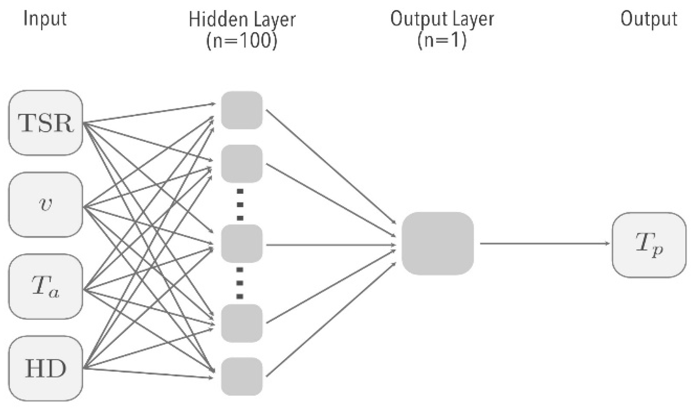
2.2. Artificial Neural Networks

ANNs are algorithms that simulate linear and non-linear processes that attempt to imitate the human brain. ANNs have the advantage that they learn the relationships between variables from historical data, and it is not necessary to have information about the physical processes involved [28].

The architecture of an ANN is composed of three main layers: one input layer, one or more hidden layers, and one output layer [39]. The number of neurons in the hidden layer depends on the particular problem and is determined by trial and error [26]. In general, a small number of neurons is not recommended [39].

The neurons $y_i$ of a layer are calculated by the summation of the previous variables $x_j$ weighted by functions ${\omega }_{ij}$ and bias $b_i$, and an activation function $\mathsf{\Phi }$, as follows:

$$y_i=\mathsf{\Phi }\left({\sum }_{j=1}^N{\omega }_{ij}{x}_j-b_i\right)$$

(4)

with N representing the number of neurons. To our knowledge, the most used activation functions are the hyperbolic tangent

$$\mathsf{\Phi }\left(x\right)={\displaystyle \frac{e^x-e^{-x}}{e^x+e^{-x}}}$$

(5)

and the sigmoid [26]

$$\mathsf{\Phi }\left(x\right)={\displaystyle \frac{1}{1-e^{-x}}}$$

(6)

Some authors have reported that the best results are obtained with only one hidden layer and that the error indicators remain constant for configurations up to five layers [39,40]. If the numbers of layers increases, accuracy falls significantly.

There are different algorithms for the ANN configuration, with back-propagation (BP) the most commonly used. The BP algorithm is a multi-layer feed-forward network that adjusts the weights and biases that modulate the connections between neurons to minimize the errors between the simulated and observed data [41].

A scheme of the ANN configuration is shown in in Figure 2. The BP algorithm was configured with one input layer with four neurons (TSR, $T_a$, $v$, and the hour of the day HD), one hidden layer containing 100 neurons, and one output layer with one variable ($T_p$). The activation function was the hyperbolic tangent defined in Equation (5). From all the available data, 50% were used for training, testing, and validating the ANN. The remaining 50% were used for predicting the panel temperature. The creation of the model and training of the ANN were performed by the MATLAB Neural Network Toolbox 2017.

Figure 2. Artificial Neural Network scheme with a single hidden layer with 100 neurons, one input layer with neurons (TSR, $T_a$, $v$), and one output layer with one neuron.

Figure 2. Artificial Neural Network scheme with a single hidden layer with 100 neurons, one input layer with neurons (TSR, $T_a$, $v$), and one output layer with one neuron.

2.3. Deterministic Models

There are many different deterministic models reported in the literature. For the purposes of this work, two main criteria were established: (a) models that include at least one atmospheric variable and (b) the models that not rely solely on the physical parameter of the PV technology used. In this work, we evaluate the panel temperature applying five analytical models, which differ in the atmospheric parameters taken into account and/or physical characteristic of the cells. According to the revision, these selected models provide the most accurate results so far because these are modifications or improvements of other widely used models.

The analytical models used in this work are represented by a mathematical expression, which relates $T_p$ with atmospheric variables. In the Standard model (SM), $T_p$ depends on $T_a$ and TSR; King’s model (KM) and Faiman’s model (FM) add the dependence of wind speed $v$, and Mattei’s (MM) and Skoplaki’s model (SkM) include the effect of the heat transfer in $h_w$. A description of these models is shown later in the text.

2.3.1. Standard Model

The SM is the first model that describes the dependence of the cell temperature on atmospheric parameters [8,13,42]. The model is valid for wind speed $v=1\mathrm{m}{\mathrm{s}}^{-1}$, and the following equation describes it:

$$T_p=T_a+{\displaystyle \frac{TSR}{{TSR}_{NOCT}}}\left(T_{NOCT}-T_{a,NOCT}\right)$$

(7)

here, $T_{NOCT}$ = 47 °C is the temperature of the cell at conditions of the nominal terrestrial environment, which corresponds to global solar radiation (GSR) and air temperature values of ${TSR}_{NOCT}$ = 800 W m⁻² and $T_{a,NOCT}$ = 20 °C, respectively.

The SM is the simplest model and does not consider cooling by the wind and other losses.

2.3.2. King’s Model

Ref. [11] developed a model to describe the cell temperature, based on two types of systems: (i) flat-plate modules mounted on an open rack, with insulated back surfaces, and (ii) concentrator modules with finned heat sinks.

KM reads as follows:

$$T_p=T_a+{TSR}_o\times e^{-\left(a+bv\right)}$$

(8)

with $a$ and $b$ coefficients that describe the effect of the radiation and wind speed, respectively, and ${TSR}_o$ is the normalized tilted radiation [15]. For the flat-plate array, the model coefficients are $a$ = 3.473 and $b$ = 0.0594 s m⁻¹.

2.3.3. Faiman’s Model

FM is inspired in the Hottel–Whillier–Bliss (HWB) equation, developed to describe the temperature of flat-plate solar thermal collectors. In [43], the authors proposed the following relationship between the panel temperature and the atmospheric variables:

$$T_p=T_a+{\displaystyle \frac{TSR}{U_0+U_{1}v}}$$

(9)

with $U_0$ (W °C⁻¹ m⁻²) and $U_1$ (W °C⁻¹ m⁻³ s) coefficients that describe the effect of the radiation and wind cooling on the cell temperature, respectively. This model did not consider the kind of technology in the values of the coefficients. On the contrary, in 2011, Koehl et al. evaluated the values $U_0$ and $U_1$ for seven different types of solar cells [15]. For pc-Si cells, he found the parameters that best fit the observations were $U_0$ = 30.02 W °C⁻¹ m⁻² and $U_1$ = 6.28 W °C⁻¹ s m⁻³.

2.3.4. Mattei’s Model

M. Mattei, 2006, proposed a model where the cell temperature depends not only on atmospheric parameters but also on the solar cell efficiency [8]. In the model, losses due to thermal processes were also included.

For pc-Si modules, the authors proposed the following equation:

$$T_p={\displaystyle \frac{U_{PV}{T}_a+TSR\left[\left(\tau \alpha \right)-\eta -\mu T_o\right]}{U_{PV}-\mu TSR}},$$

(10a)

where $U_{PV}$ (W m⁻² °C⁻¹) is the heat exchange coefficient; $\tau \alpha$ is the fraction of radiation absorbed by the cell; $\eta$ is the cell efficiency at standard conditions, i.e., at panel temperature $T_o$ = 25 °C and $TSR$ = 1000 W m⁻²; and $\mu$ (°C⁻¹) is the temperature coefficient. The influence of wind and forced thermal convection losses are included through the coefficient $U_{PV}$.

There is a wide discrepancy in the $U_{PV}$ values [44,45]. In this work, we used the linear relationship between $U_{PV}$ and wind speed proposed by [8]:

$$U_{PV}=26.6\left(\mathrm{W}{\mathrm{m}}^2{°\mathrm{C}}^{-1}\right)+2.3\left(\mathrm{W}{\mathrm{m}}^2{°\mathrm{C}}^{-1}\mathrm{s}\right)v$$

(10b)

Besides, the authors used the following values for the parameters: $\tau \alpha$ = 0.81, ${\eta }_r$ = 0.125, $\mu$ = 0.0005 °C⁻¹.

2.3.5. Skoplaki’s Model

Similar to MM, E. Skoplaki, 2008, developed a model where the cell temperature depends on atmospheric parameters and heat transfer [12]. The authors proposed the following equation:

$$T_p=T_a+\left({\displaystyle \frac{TSR}{{TSR}_{NOCT}}}\right){\displaystyle \frac{h_{w,NOCT}}{h_w}}\left(T_{NOCT}-T_{a,NOCT}\right)\left[1-{\displaystyle \frac{\eta }{\tau \alpha }}\left(1+{\displaystyle \frac{\mu }{\eta }}{T}_o\right)\right]$$

(11a)

here, $h_w$ (W m⁻² K⁻¹) and $h_{w,NOCT}$ (W m⁻² K⁻¹) are the wind convection heat transfer coefficient and the wind convection heat transfer coefficient at nominal terrestrial conditions, respectively.

For pc-Si cells, [12] found the following values for the model’s parameters: $h_{w,NOCT}$ = 10.91 W m⁻² K⁻¹, $\tau \alpha$ = 0.9, $\mu$ = 0.00048 °C⁻¹, and $\eta$ = 0.12. Further, the wind convection heat transfer coefficient depends linearly on the wind speed:

$$h_w=8.91\left(W{m}^{-2}{K}^{-1}\right)+2.0\left(W{m}^{-3}s{K}^{-1}\right)v$$

(11b)

3. Results and Discussion

3.1. Local Meteorological Characteristics and Temperature of the Panel

In this section, we analyzed the meteorological characteristics in Luna based on data collected over two years. The analyzed variables were GSR, TSR, air temperature ($T_a$), panel temperature ($T_p$) wind speed (v), and wind direction. The analysis was based on data registered in Luna, except for wind direction, taken from the station at Vicuña.

3.1.1. Solar Radiation

The maximum values of GSR and TSR were 1249 W m⁻² and 1246 W m⁻², respectively, both registered on 28 December 2016 at 13:00 LT. Figure 3a displays the mean monthly behavior of these two variables. As a reference, we indicate the minimum zenith angle, i.e., the sun’s angular distance to the zenith at noon. For details about the definition of the zenith angle, see [46].

The mean monthly values of GSR ranged between 123.9 W m⁻² and 332.8 W m⁻², reached in June and December, respectively. TSR fluctuated between 166.5 W m⁻² and 309.5 W m⁻² in May and December, respectively. Figure 3a shows that for most of the year, TSR is higher than GSR. Nevertheless, in summer, the opposite occurs because the sun is closer to the zenith than in winter. The closest distance to the zenith is 6.7°, and it occurs in December during the summer solstice.

Figure 3b shows the mean daily cycle of GSR and TSR. On average, during the daylight hours, TSR is higher than GSR. These results are consistent with the values of GSR in the Elqui Valley reported by [35].

Figure 3. Meteorological characteristics of Luna. (a) Mean monthly evolution of GSR (black) and TSR (gray). The dashed line represents the minimum zenith angle. (b) Mean daily cycle of GSR (black) and TSR (gray). (c) Mean monthly evolution of air (black) and panel (gray) temperature. (d) Mean daily cycle of air (black) and panel (gray) temperature. (e) Wind direction distribution in Vicuña. (f) Mean daily cycle of wind speed.

Figure 3. Meteorological characteristics of Luna. (a) Mean monthly evolution of GSR (black) and TSR (gray). The dashed line represents the minimum zenith angle. (b) Mean daily cycle of GSR (black) and TSR (gray). (c) Mean monthly evolution of air (black) and panel (gray) temperature. (d) Mean daily cycle of air (black) and panel (gray) temperature. (e) Wind direction distribution in Vicuña. (f) Mean daily cycle of wind speed.

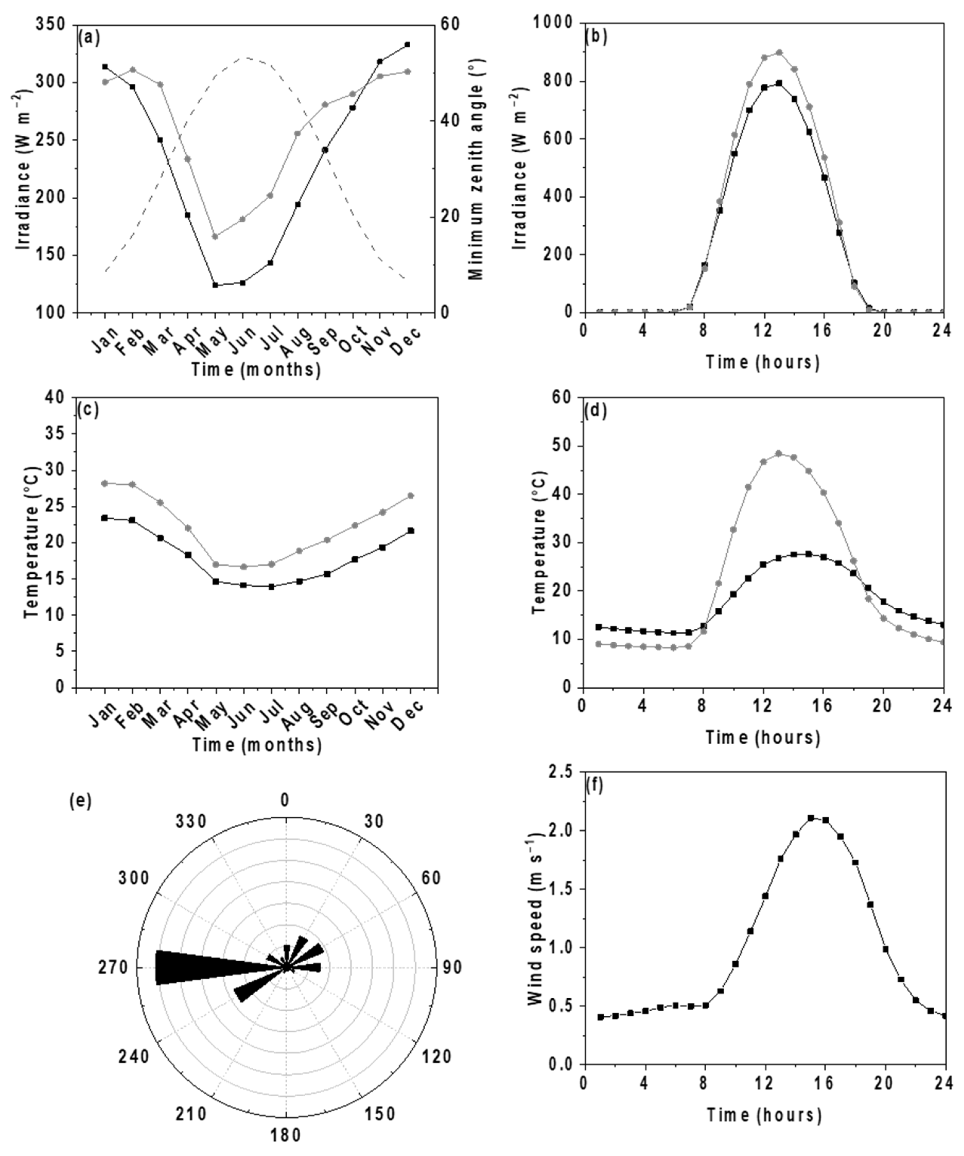
3.1.2. Air and Panel Temperature

The values of $T_a$ fluctuated between 0.9 °C and 37.9 °C, reached on 12 May 2017 at 02:00 LT, and 26 December 2015 at 15:00 LT, respectively. For $T_p$, the minimum and maximum values were −2.6 °C and 64.0 °C on 16 July 2017 at 08:00 LT and 21 August 2016 at 14:00 LT, respectively.

Figure 3c shows the mean monthly behavior of air and panel temperature. We found that the maximum values were 23.4 °C and 28.2 °C for $T_a$ and $T_p$, respectively, both reached in January; meanwhile, the minimum of $T_a$ and $T_p$ was 13. 9 °C and 16.7 °C, achieved in July and June, respectively.

Figure 3d depicts the mean daily cycle of air and panel temperature. On average, during the day hours, $T_p$ is higher than $T_a$, which is consistent with the results found by [47]. During the night, the behavior is the opposite. The mean daily values of $T_a$ varied between 11.3 °C and 27.6 °C at 06:00 LT and 16:00 LT, respectively. In the case of $T_p$, the minimum and maximum values were 8.3 °C and 48.5 °C at 07:00 LT and 14:00, respectively. The low values of $T_p$ during the night can be a consequence of the cooling due to thermal radiation [48].

3.1.3. Wind Velocity

The wind is thermic induced: during the day, westerly winds are observed, and at night, the wind blows in the opposite direction. We can see this characteristic of the wind direction in Figure 3e.

The wind speed reached values of up to 4.7 m s⁻¹ on 21 November 2016 at 08:00 LT. The mean monthly values are higher in summer than in winter, ranging between 0.8 m s⁻¹ and 1.2 m s⁻¹ in May and January, respectively.

Figure 3f depicts the mean daily cycle of wind speed. The figure shows that during the day, wind speed is higher than during the night. On average, the maximum value of wind speed was 2.1 m s⁻¹ at 15:00 LT. These characteristics of the wind velocity are consistent with the results found by [35] in the Elqui Valley.

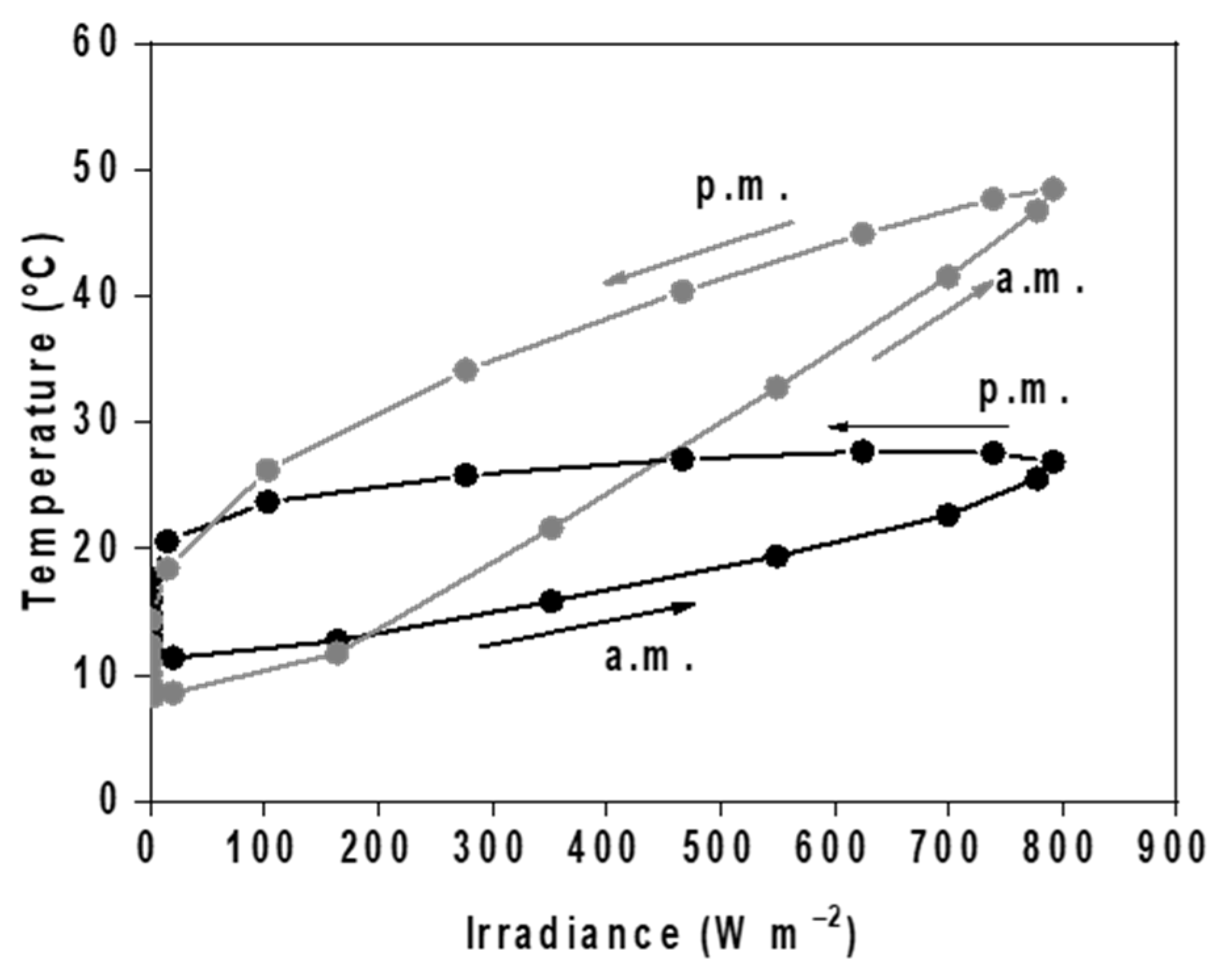
3.1.4. Relationships between Atmospheric Variables and Panel Temperature

The atmospheric variables measured at a weather station are not independent but also are related to each other in a complex non-linear way. This fact can be observed in Figure 4, where we can see the relationships between all pairs of variables considered in this study.

Figure 4. Relationships between variables. (a) Air temperature vs. tilted solar radiation; (b) panel temperature vs. air temperature; (c) panel temperature vs.; (d) wind speed vs. air temperature; (e) wind speed vs. panel temperature; (f) wind speed vs. tilted solar radiation.

Figure 4. Relationships between variables. (a) Air temperature vs. tilted solar radiation; (b) panel temperature vs. air temperature; (c) panel temperature vs.; (d) wind speed vs. air temperature; (e) wind speed vs. panel temperature; (f) wind speed vs. tilted solar radiation.

In Figure 4a, we observe that $T_a$ tends to rise with TSR, which can be explained because, during daytime, solar radiation warms the ground, causing the heating of the air.

Figure 4b,c display the panel temperature dependence on $T_a$ and TSR, respectively. We observe that $T_p$ tends to rise with air temperature and solar radiation because the two variables contribute to heat the panel. These results are consistent with Figure 3 and Figure 4, which show that the mean daily cycle of these three variables follows the same trend.

Figure 4d,e and f exhibit wind speed dependence on $T_a$, $T_p$, and TSR, respectively. The figures show a high dispersion of the data because wind speed dependence on the local atmospheric variables is more complex. The surface wind in the Elqui Valley is thermally induced [35], i.e., caused by horizontal temperature differences. Consequently, it depends not only on the local meteorological characteristics but also on the surrounding. Figure 4d,e show that wind speed tends to rise with air temperature and consequently with the panel temperature, which consistent with Figure 3. Figure 4f shows no clear relationship between wind speed and TSR.

Figure 5 shows the mean daily cycle of $T_a$ and $T_p$ as a function of TSR. We can observe that $T_a$ and $T_p$ are higher in the afternoon than in the morning for the same TSR values, so a hysteresis effect occurs. This phenomenon has been previously reported by other authors [49,50].

Figure 5. Mean daily cycle of the air and panel temperature as a function of TSR. Black: air temperature; gray: panel temperature.

Figure 5. Mean daily cycle of the air and panel temperature as a function of TSR. Black: air temperature; gray: panel temperature.

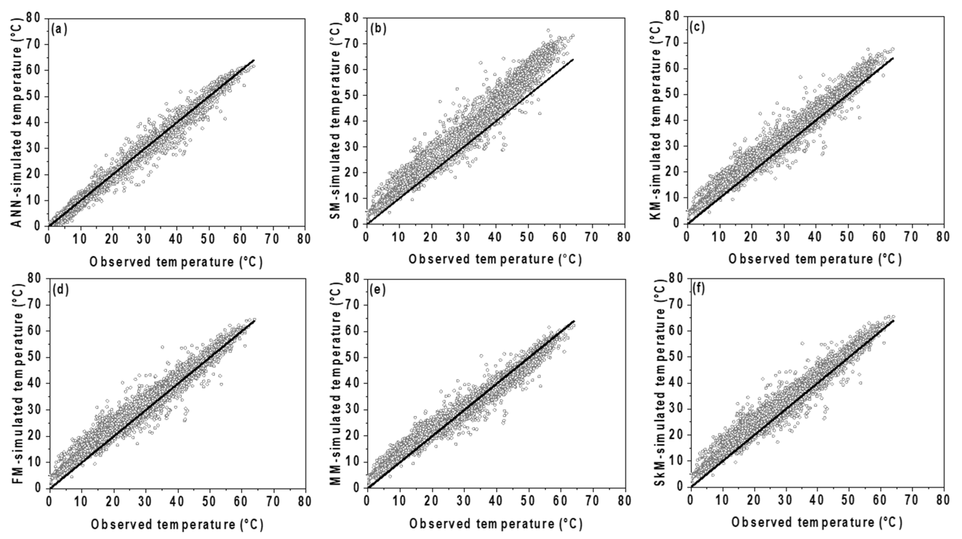
3.2. Prediction of the Panel Temperature

In this section, we analyze the panel temperature prediction from atmospheric variables using an ANN and the five deterministic models, described in Section 2.2 and Section 2.3. For the deterministic models, represented by Equations (7)–(11), we used the parameters recommended by the authors. In the case of FM, we take the values of the parameters $U_o$ and $U_1$ proposed by M. Koehl, 2011 [15]; in MM and SkM, we utilized Equations (10b) and (11b) for the heat exchange coefficient $U_{PV}$, and wind convection heat transfer coefficient $h_w$, respectively.

From the two-year data available, we take one year (October 2015 to September 2016) to train the ANN. So, the presented results are based on one-year data, from October 2016 to September 2017. After gathering information provided by the owners, the operational conditions of the PV park did not change between the training and testing period.

Figure 6a shows the relationship between $T_p$ simulated with the ANN and the observations. The plot shows that the observed and simulated data are homogeneously distributed around the straight identity. The naked eye does not appreciate an overestimation or underestimation.

Figure 6. Panel temperature simulated (vertical axis) and observed (horizontal axis). The solid line represents the identity curve. (a) ANN; (b) SM; (c) KM; (d) FM; (e) MM; (f) SkM.

Figure 6. Panel temperature simulated (vertical axis) and observed (horizontal axis). The solid line represents the identity curve. (a) ANN; (b) SM; (c) KM; (d) FM; (e) MM; (f) SkM.

Figure 6b–f depict the relationship between the deterministic models and observations. The pictures show that, except for MM, the models tend to overestimate observations. In the MM case, Figure 6e shows an overestimation for $T_p$ < 30 °C and an underestimation for $T_p$ > 40 °C.

To evaluate the level of agreement between the models and observations, we calculate the errors using three metrics.

Table 1. R, MBE and RMSE of ANN and deterministic models.

Model	Atmospheric Variables	R	MBE (°C)	RMSE (°C)
ANN	-	1.00	−0.11	1.59
SM	Ta, TSR	0.99	4.72	5.83
KM	Ta, TSR, v	0.99	3.23	3.98
FM	Ta, TSR, v	0.99	2.44	3.56
MM	Ta, TSR, v	0.99	1.85	3.30
SkM	Ta, TSR, v	0.99	2.70	3.73

shows the R, MBE, and RMSE values for the ANN and the deterministic models. For clarity, the atmospheric variables considered in the analytical model are also shown.

In the case of R, we found that for the ANN model, the coefficient was 1.00, whereas for all deterministic models, the value was 0.99. This means that regarding the used variables to predict $T_p$, both the ANN and the deterministic models are highly correlated. On the other hand, the MBE for the ANN model is −0.11 °C, meaning a slight underestimation of the data. The MBE values for all deterministic models were positive, which indicates a trend to overestimate the observations. Among the deterministic models, MM presents the lowest MBE. These findings are consistent with Figure 7.

Figure 7. Hourly MBE (a) and RMSE (b) of ANN and deterministic models.

Figure 7. Hourly MBE (a) and RMSE (b) of ANN and deterministic models.

Concerning the RMSE, the ANN is the model with the lowest value, which indicates the ANN’s superiority over the deterministic models to predict the panel temperature from historical data. Among the deterministic models, MM presents the lowest RMSE value, consistent with the previously reported results by [17].

A more detailed view of each model’s performance to predict $T_p$ can be obtained, analyzing the hourly MBE and RMSE, shown in Figure 7. Figure 7a shows that the hourly MBE for the ANN model oscillated around 0 °C during the whole day. This behavior is significantly different from the one exhibited by the deterministic models. During the night hours, when TSR is zero, all models predict the same values. This result is expected because the models predict that $T_p$ matches $T_a$ for TSR zero, meaning that these models do not simulate the night-time radiative cooling of the panels, shown in Figure 3d.

During the daylight hours, the MBE of each deterministic model exhibits different behavior. Figure 7a shows that the model that differs the most from the observations is SM, which can be attributed to the fact that it does not consider cooling by the wind and convective processes. The other four models, during the morning overestimated the observations, reaching the highest MBE between 8:00 LT and 9:00 LT. This overestimation could be due to heat exchange processes not considered in the models. After this time, the MBE decreases, which coincides with the increase in wind speed (see Figure 5). These findings show that except for SM, the deterministic models can incorporate, to some extent, the effect of the wind’s cooling on $T_p$. The KM is capable of incorporating the cooling by the wind speed, but it always overestimates $T_p$. FM, MM, and SkM exhibit similar behavior: in the morning, they overestimate the observations, and after some time point, the opposite occurs. When TSR = 0, all deterministic models match, predicting that $T_p$ and $T_a$ coincide. In the morning, MM stands out as the one that best predicts $T_p$, and from 15:00 LT to 17:00 LT, SkM is the best fitting one.

Figure 7b shows the hourly RMSE for the ANN and deterministic models. It can be seen that the ANN model exhibits the lowest value during almost the whole day, with a maximum RMSE of 2.69 °C at 13:00 LT. The evolution of the RMSE of the deterministic models is similar: as the hours of the day progress, it reaches a maximum, decreasing afterward until reaching the minimum when TSR = 0. The peak value for the SM shifts to 13:00 LT, also when TSR and $T_a$ are maximum (see Figure 3d), which could be because this model does not consider cooling processes. Regarding the deterministic models that include wind speed, the RMSE decreases after 9:00 LT when the wind blows (Figure 3f).

Further, we can see in Figure 7 that, after midday, the RMSE for the ANN model is similar to those for MM, FM, and SkM. In the afternoon, FM and SkM present an RMSE slightly lower than the ANN model.

It is interesting to observe that, for the ANN, the daily RMSE behavior in the morning is similar to that observed in the afternoon, which does not happen in the deterministic models. This effect could be because the ANN considers the day’s hour in training, meaning that it considers, to some extent, the hysteresis effect shown in Figure 5.

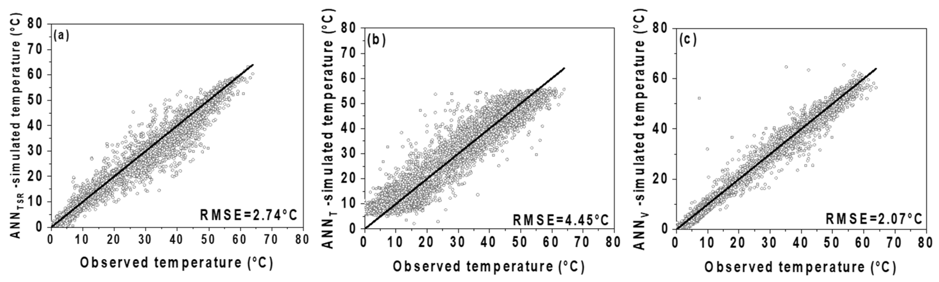
3.3. Sensitivity of Panel Temperature on Air Temperature, Tilted Solar Radiation, and Wind Speed

To analyze the sensitivity of the panel temperature regarding the atmospheric variables, we trained three new ANNs, as described in Section 2.2, but excluded one variable in training:

• ANN_TSR: TSR is excluded;
• ANN_T: $T_a$ is excluded;
• ANN_v: $v$ is excluded.

The relationship between the simulated and observed $T_p$ for the three cases are represented in Figure 8. It is possible to observe that the ANN_T and ANN_v models exhibited the highest and lowest data dispersion, respectively. These results are in line with the RMSE values showed in the figure.

Figure 8. Panel temperature simulated (vertical axis) and observed (horizontal axis). The solid line represents the identity curve. (a) ANN_TSR; (b) ANN_T; (c) ANN_v.

Figure 8. Panel temperature simulated (vertical axis) and observed (horizontal axis). The solid line represents the identity curve. (a) ANN_TSR; (b) ANN_T; (c) ANN_v.

To quantify the impact of the atmospheric variables on $T_p$, we define the Exclusion Importance Index (EII) as the normalized RMSE between $T_p$ simulated from the new ANNs and the observations (see

Table 2. Exclusion Importance Index (EII) and Permutation Feature Importance (PFI).

Variable	EII	PFI
Air temperature	0.48	0.51
Tilted solar radiation	0.30	0.47
Wind speed	0.22	0.02

). The higher the EII, the higher the importance of the variable on the panel temperature.

Figure 9 displays the daily cycle of the hourly MBE and RMSE for the three models. From Figure 9a, we observed that during the daylight hours, the MBE was positive for ANN_T and negative for ANN_TSR. Accordingly, when $T_a$ and TSR are not considered, the ANN model over- and sub-estimates the mean panel temperature, respectively. During the night, in both cases, the MBE values are near zero. For the ANN_v model, the MBE values remain around zero all day. These results are consistent with the mean daily cycle of $T_p$.

Figure 9. (a) Daily cycle of MBE and (b) RMSE. In both graphics, solid line: ANN_TSR, dotted line: ANN_T, dashed line: ANN_v.

Figure 9. (a) Daily cycle of MBE and (b) RMSE. In both graphics, solid line: ANN_TSR, dotted line: ANN_T, dashed line: ANN_v.

Figure 9b shows that ANN_T presents the highest hourly RMSE during the whole day. During the night, ANN_T is the only one that exhibited significant values because there was neither radiation nor wind. Other authors have reported that air temperature, solar radiation and humidity are the most important variables for predicting the panel temperature [20,32]. However, the relative impact of these variables on the panel temperature is strongly affected by the local geographical characteristics [17].

Several authors analyze the sensitivity of the input variables on output one using the Permutation Feature Importance (PFI) Index. PFI is calculated using the original ANN but permuting the values of the variable under study. PFI is defined as the normalized Mean Square Error [51]. The higher the PFI, the higher the importance of the variable.

The sensitivity analysis was carried out by calculating the EII and PFI. As observed in Table 2, both methods are consistent: the variable with the highest and lowest impact on the panel temperature is the air temperature and wind speed, respectively.

The results shown in this section indicate that, from the analyzed atmospheric variables, the air temperature is the one that influences the panel temperature the most, followed by solar radiation and wind speed.

4. Conclusions

In this work, we used Artificial Neural Networks (ANNs) to predict the panel temperature $T_p$ from solar radiation TSR, air temperature $T_a,$ and wind speed $v$. The study was based on data registered in an operative photovoltaic park located in the semi-arid north of Chile. The simulated results were compared with five deterministic models using three error metrics, namely the correlation coefficient (R), the mean bias (MBE), and the Root Mean Square Error (RMSE). We also used ANNs for analyzing the relative impact of TSR, $T_a$ and $v$ on $T_p$.

Our main findings are as follows:

(1)

The ANN model presents a slight underestimation of the panel temperature; meanwhile, all deterministic models show a visible overestimation. The ANN reached the highest R, the smallest MBE, and the smallest RMSE.

(2)

The correlation coefficient was higher than 0.99 both for the ANN and deterministic models, meaning that all models can simulate the correlation between panel temperature and atmospheric variables.

(3)

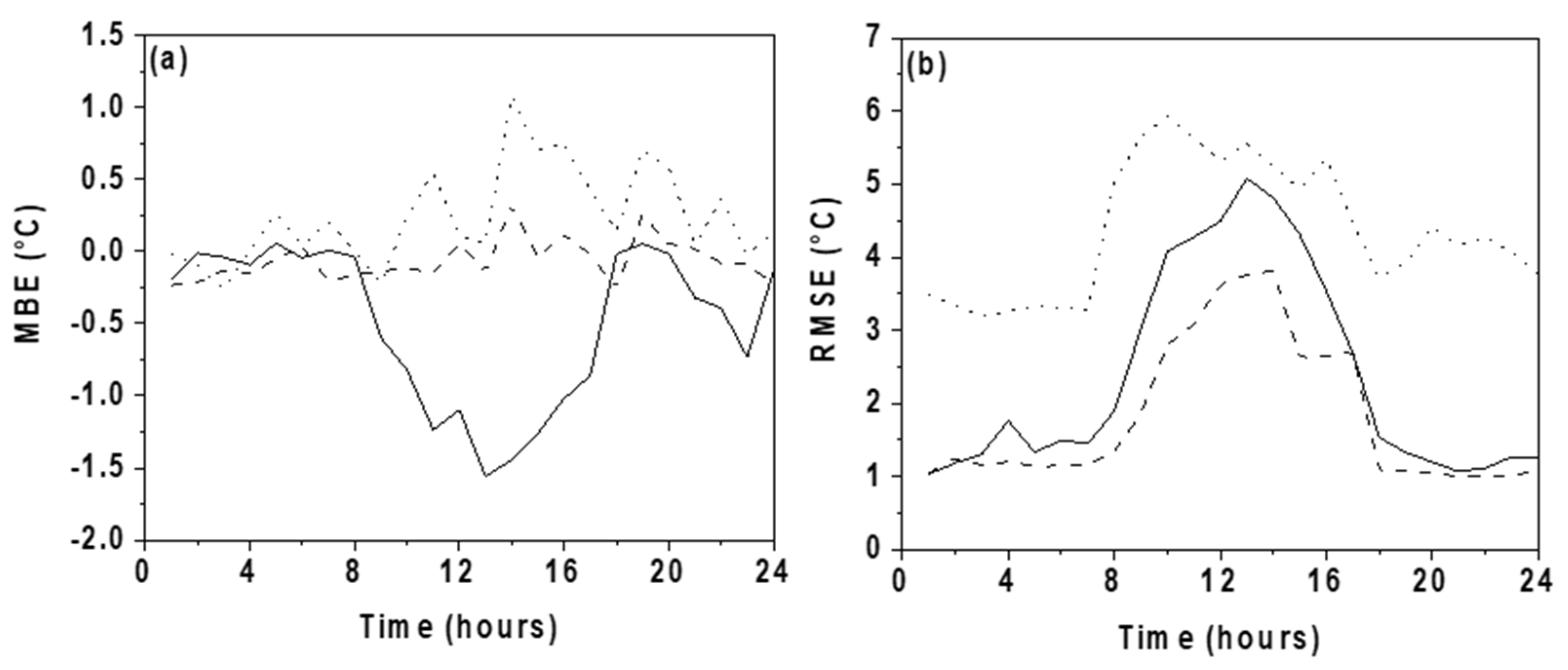
The ANN is the model that best predicts the mean daily behavior of $T_p$ during most of the day, except in the afternoon, when the hourly RMSE is similar to Mattei’s and King’s models.

(4)

The ANN is the only model that can predict the night cooling of the panels.

These findings indicate the superiority of the ANN over deterministic models to predict the panel temperature from atmospheric variables.

(5)

During the day, all deterministic models, except the Standard model, exhibit a decrease in the RMSE when the wind blows, indicating that the inclusion of wind plays an important role in the estimation of $T_p$. Among the deterministic models, Mattei’s model is the one that performs best.

(6)

Among the analyzed variables, $T_a$ has the highest impact on the panel temperature, followed by TSR and wind speed. This suggests that the atmospheric variable that influences the panel temperature for semi-arid regions with low humidity the most is air temperature.

ANNs learn the relationships between variables from historical data. In the case analyzed here, the panel temperature depends not only on atmospheric variables but also on other factors such as technology (electronic parameters, topography, the size of the PV park, etc.). These relationships are implicit in the historical data, and so the ANN learns it. Therefore, although the methodology shown in this article can be applied for any PV system, the ANN must be trained with data registered on the particular park and place.

So, this work demonstrates the capability of ANNs to simulate the complex physical processes involved in the interaction between photovoltaic panels and atmospheric variables.

References

1. Tahmineh, M.; Wang, Y.; Hahn, Y. Graphene and its derivatives for solar cells applications. Nano Energy 2018, 47, 51–65. [Google Scholar]
2. Coordinador Eléctrico Nacional. Available online: https://www.coordinador.cl/ (accessed on 10 April 2024).
3. Henríquez, M.; Guerrero, L.; Fernández, A.; Fuentealba, E. Lithium nitrate purity influence assessment in ternary molten salts as thermal energy storage material for CSP plants. Renew. Energy 2020, 149, 940–950. [Google Scholar] [CrossRef]
4. Cordero, R.; Damiani, A.; Laroze, D.; Macdonell, S.; Jorquera, J.; Sepúlveda, E.; Feron, S.; Llanillo, P.; Labbe, F.; Carrasco, J.; et al. Effects of soiling on photovoltaic (PV) modules in the Atacama Desert. Sci. Rep. 2018, 8, 13943. [Google Scholar] [CrossRef] [PubMed]
5. El Amin, A.; Al-Maghrabi, M. The analysis of temperature effect for mc-Si photovoltaic cells performance. Silicon 2018, 10, 1551–1555. [Google Scholar] [CrossRef]
6. Yolcan, O.O.; Kose, R. Photovoltaic module cell temperature estimation: Developing a novel expression. Sol. Energy 2023, 249, 1–11. [Google Scholar] [CrossRef]
7. Chintapalli, N.; Sharma, K.M.; Bhattacharya, J. Linking spectral, thermal and weather effects to predict location-specific deviation from the rated power of a PV panel. Sol. Energy 2020, 208, 115–123. [Google Scholar] [CrossRef]
8. Mattei, M.; Notton, G.; Cristofari, C.; Muselly, M.; Poggi, P. Calculation of the polycrystalline PV module temperature using a simple method of energy balance. Renew. Energy 2006, 31, 553–567. [Google Scholar] [CrossRef]
9. May-Tzuc, O.; Bassam, A.; Mendez-Monroy, P.E.; Sanchez Dominguez, I. Estimation of the operating temperature of photovoltaic modules using artificial intelligence techniques and global sensitivity analysis: A comparative approach. J. Renew. Sustain. Energy 2018, 10, 033503. [Google Scholar] [CrossRef]
10. Elminshawy, N.A.S.; El Ghandour, M.; Gad, H.M.; El-Damhogi, D.G.; El-Nahhas, K.; Addas, M.F. The performance of a buried heat exchanger system for PV panel cooling under elevated air temperature. Geothermics 2019, 82, 7–15. [Google Scholar] [CrossRef]
11. Photovoltaic Array Performance Model. Available online: https://energy.sandia.gov/wp-content/gallery/uploads/043535.pdf (accessed on 22 July 2024).
12. Skoplaki, E.; Boudouvis, A.; Palyvos, J. A simple correlation for the operating temperature of photovoltaics modules of arbitrary mounting. Sol. Energy Mater. Sol. Cells 2008, 52, 1393–1402. [Google Scholar] [CrossRef]
13. Skoplaki, E.; Palyvos, J. Operating temperature of photovoltaic modules: A survey of pertinent correlations. Renew. Energy 2009, 34, 23–29. [Google Scholar] [CrossRef]
14. Kurtz, S.; Whitfield, K.; Miller, D.; Joyce, J.; Wohlgemuth, J.; Kempe, M.; Dhere, N.; Bosco, N.; Sgonena, T. Evaluation of high-temperature exposure of rack-mounted photovoltaic modules. In Proceedings of the 34th IEEE Photovoltaic Specialist Conference, Philadelphia, PA, USA, 7–12 June 2009; pp. 2399–2404. [Google Scholar]
15. Koehl, M.; Heck, M.; Weismeier, S.; Wirth, J. Modelling of the nominal operating cell temperature based on outdoor weathering. Sol. Energy Mater. Sol. Cells 2011, 95, 1638–1646. [Google Scholar] [CrossRef]
16. Ayvazoğluyüksel, O.; Filik, Ü. Estimation methods of global solar radiation, cell temperature and solar power forecasting: A review and case study in Eskisehir. Renew. Sustain. Energy Rev. 2018, 91, 639–653. [Google Scholar] [CrossRef]
17. Schwingshackl, C.; Petitta, M.; Wagner, J.; Belluardo, G.; Moser, D.; Castelli, M.; Zebisch, M.; Tetzlaff, A. Wind effect on PV module temperature: Analysis of different technics for an accurate estimation. Energy Procedia 2013, 40, 77–86. [Google Scholar] [CrossRef]
18. Kaplani, E.; Kaplanis, S. Dynamic Electro-Thermal PV Temperature and Power Output Prediction Model for any PV Geometries in Free-Standing and BIPV Systems Operating under any Environmental Conditions. Energies 2020, 13, 4743. [Google Scholar] [CrossRef]
19. Khandakar, A.; Chowdhury, M.; Kazi, M.; Benhmed, K.; Touati, F.; Al-Hitmi, M.; Gonzales, A. Machine learning based photovoltaics (PV) power prediction using different environmental parameters of Qatar. Energies 2019, 12, 2782. [Google Scholar] [CrossRef]
20. Pasion, C.; Wagner, T.; Koscgnick, C.; Schuldt, S.; Williams, J.; Hallinam, K. Machine learning modeling of horizontal photovoltaic using weather and location data. Energies 2020, 13, 2570. [Google Scholar] [CrossRef]
21. Yousif, J.; Kazem, H.; Alattar, N.; Elhassan, I. A comparison study based on artificial neural networks for assessing PV/T solar energy production. Case Stud. Therm. Eng. 2019, 13, 100407. [Google Scholar] [CrossRef]
22. Rodríguez-Romero, J.A.; Mendoza-Castillo, D.I.; Reynel-Ávila, H.E.; de Haro-Del Rio, D.A.; González-Rodríguez, L.M.; Bonilla-Petriciolet, A.; Durán-Valle, C.J.; Camacho-Aguilar, K.I. Preparation of a new adsorbent for the removal of arsenic and its simulation with artificial neural network-based adsorption models. J. Environ. Chem. Eng. 2020, 8, 103928. [Google Scholar] [CrossRef]
23. Manobel, B.; Sehnke, F.; Lazzus, J.; Salfate, I.; Felder, M.; Montecinos, S. Wind turbine power curve modeling based on Gaussian Processes and Artificial Neural Networks. Renew. Energy 2018, 125, 1015–1020. [Google Scholar] [CrossRef]
24. Salfate, I.; Marin, J.C.; Cuevas, O.; Montecinos, S. Improving wind speed forecasts from the Weather Research and Forecasting model at a wind farm in the semiarid Coquimbo region in central Chile. Wind Energy 2020, 23, 1939–1954. [Google Scholar] [CrossRef]
25. Barrera, J.M.; Reina, A.; Maté, A.; Trulijjo, J.C. Solar Energy Prediction Model Based on Artificial Neural Networks and Open Data. Sustainability 2020, 12, 6915. [Google Scholar] [CrossRef]
26. Lo Brano, V.; Ciulla, G.; Di Falco, M. Artificial Neural Networks to Predict the Power Output of a PV Panel. Int. J. Photoenergy 2014, 2014, 193083. [Google Scholar] [CrossRef]
27. Fouilloy, A.; Voyant, C.; Notton, G.; Motte, F.; Paoli, C.; Nivet, M.; Guillot, E.; Duchaud, J. Solar irradiation prediction with machine learning: Forecasting models selection method depending on weather variability. Energy 2018, 165, 620–629. [Google Scholar] [CrossRef]
28. Sulaiman, S.I.; Zainol, N.Z.; Othman, Z.; Zainuddin, H. Cuckoo Search for Determining Artificial Neural Network Training Parameters in Modeling Operating Photovoltaic Module Temperature. In Proceedings of the International Conference on Modelling, Identification & Control, Grindelwald, Switzerland, 23–25 February 2004. [Google Scholar]
29. Ciulla, G.; Lo Brano, V.; Moreci, E. Forecasting the Cell Temperature of PV Modules with an Adaptive System. Int. J. Photoenergy 2013, 2013, 192854. [Google Scholar] [CrossRef]
30. Dzib, J.T.; Moo, E.J.A.; Bassam, A.; Flota-Bañuelos, M.; Soberanis, E.; Ricaldi, L.J.; López-Sánchez, J. Photovoltaic Module Temperature Estimation: A Comparison between Artificial Neural Networks and Adaptive Neuro Fuzzy Inference Systems Models. In Intelligent Computing Systems, ISICS, Communications in Computer and Information Science; Martin-Gonzalez, A., Uc-Cetina, V., Eds.; Springer: Cham, Switzerland, 2016. [Google Scholar]
31. Fernández, E.; Almonacid, F.; Rodrigo, P.; Perez-Higueras, P. Calculation of the cell temperature of a high concentrator photovoltaic (HCPV) module: A Study of Comparison of Different Methods. Sol. Energy Mater. Sol. Cells 2014, 121, 144–151. [Google Scholar] [CrossRef]
32. Chayapathy, V.; Anitha, G.; Raghavendra, S.; Vijaykumar, R. Solar panel temperature prediction by artificial neural networks. In Proceedings of the 4th International Conference on Recent Trends on Electronic, Information, Communication & Technology, Bengaluru, India, 17–18 May 2019. [Google Scholar]
33. Garreaud, R.; Muñoz, R. The low-level jet off West coast of subtropical South America: Structure and variability. Mon. Weather Rev. 2005, 133, 2246–2261. [Google Scholar] [CrossRef]
34. Montecinos, S.; Gutiérrez, J.; López-Cortés, F.; López, D. Climatic characteristics of the semi-arid Coquimbo Region in Chile. J. Arid Environ. 2016, 126, 7–11. [Google Scholar] [CrossRef]
35. Kalthoff, N.; Bischoff-Gauss, I.; Fiebig-Wittmaack, M.; Fiedler, F.; Thürauf, J.; Novoa, E.; Pizarro, C.; Gallardo, L.; Rondanelli, R.; Kohler, M. Mesoscale wind regimes in Chile at 30 °C. J. Appl. Meteorol. 2002, 41, 953–970. [Google Scholar] [CrossRef]
36. Olivares, S.; Squeo, F. Patrones fenológicos en especies arbustivas del desierto costero del norte-centro de Chile (Phenological stock in shrub species of the coastal desert of north-central Chile). Rev. Chil. Hist. Nat. 1999, 72, 353–370. [Google Scholar]
37. Kalthoff, N.; Fiebig-Wittmaack, M.; Meissner, C.; Kohler, M.; Uriarte, M.; Bischoff-Gauss, I.; Gonzales, E. The energy balance, evapotranspiration and nocturnal dew deposition of an arid valley in the Andes. J. Arid Environ. 2006, 65, 420–443. [Google Scholar] [CrossRef]
38. Centro de Estudios Avanzados en Zonas Áridas. Available online: www.ceazamet.cl (accessed on 10 April 2024).
39. Arifin, F.; Robbani, H.; Annisa, T.; Ma’arof, N. Variations in the number of layers and the number of neurons in artificial neural networks: Case study of pattern recognition. J. Phys. Conf. Ser. 2019, 1413, 012016. [Google Scholar] [CrossRef]
40. Fausset, L. Simple Neural Nets for Pattern Classification. In Fundamentals of Neural Networks: Architectures, Algorithms, and Applications; Prentice-Hall, Inc.: Hoboken, NJ, USA, 2014. [Google Scholar]
41. Goh, A. Back propagation neural networks for modeling complex systems. Eng. Appl. Artif. Intell. 1995, 9, 143–151. [Google Scholar] [CrossRef]
42. Markvart, T. Environmental Impacts of Photovoltaics. In Solar Electricity, 2nd ed.; John Wiley & Sons Ltd.: Chichester, UK, 2000. [Google Scholar]
43. Faiman, D. Assessing the outdoor operating temperature of photovoltaic modules. Prog. Photovolt. 2008, 16, 307–315. [Google Scholar] [CrossRef]
44. Jones, A.; Underwood, C. A thermal model for photovoltaic system. Sol. Energy 2001, 70, 349–359. [Google Scholar] [CrossRef]
45. Sandnes, B.; Rekstadt, J. A photovoltaic/thermal (PV/T) collector with polymer absorber plate, experimental study and analytical model. Sol. Energy 2002, 72, 63–73. [Google Scholar] [CrossRef]
46. Brasseur, G.; Solomon, S. Solar radiation at the top of the Atmosphere. In Aeronomy of the Middle Atmosphere: Chemistry and Physics of the Stratosphere and Mesosphere; Springer: Dordrecht, The Netherlands, 2005. [Google Scholar]
47. Husain, M.A.; Khan, Z.A.; Tariq, A. A novel solar PV MPPT scheme utilizing the difference between panel and atmospheric temperature. Renew. Energy Focus 2017, 19–20, 11–22. [Google Scholar]
48. Zhao, B.; Hu, M.; Ao, X.; Huang, X.; Ren, X.; Pei, G. Conventional photovoltaic panel for nocturnal radiative cooling and preliminary performance analysis. Energy 2019, 175, 677–686. [Google Scholar] [CrossRef]
49. Ma, T.; Yang, H.; Lu, L. Long term performance analysis of a standalone photovoltaic system under real conditions. Appl. Energy 2017, 201, 320–331. [Google Scholar] [CrossRef]
50. Du, Y.; Fell, C.J.; Duck, B.; Chen, D.; Liffman, K.; Zhang, Y.; Gu, M.; Zhu, Y. Evaluation of photovoltaic panel temperature in realistic scenarios. Energy Convers. Manag. 2016, 108, 60–67. [Google Scholar] [CrossRef]
51. Cava, W.; Bauer, C.; Moore, J.H.; Pendergrass, S.A. Interpretation of machine learning predictions for patient outcomes in electronic health records. Proc. AMIA Annu. Symp. 2020, 2019, 572–581. [Google Scholar]
Figure 1. Location of the studied area and Luna PV park. The gray colors represent the altitude according to the scale shown on the right side of the figure. Contour lines are each 300 m.
Energies 17 05844 g001