Optimizing Models and Data Denoising Algorithms for Power Load Forecasting

Abstract

To handle the data imbalance and inaccurate prediction in power load forecasting, an integrated data denoising power load forecasting method is designed. This method divides data into administrative regions, industries, and load characteristics using a four-step method, extracts periodic features using Fourier transform, and uses Kmeans++ for clustering processing. On this basis, a Transformer model based on an adversarial adaptive mechanism is designed, which aligns the data distribution of the source domain and target domain through a domain discriminator and feature extractor, thereby reducing the impact of domain offset on prediction accuracy. The mean square error of the Fourier transform clustering method used in this study was 0.154, which was lower than other methods and had a better data denoising effect. In load forecasting, the mean square errors of the model in predicting long-term load, short-term load, and real-time load were 0.026, 0.107, and 0.107, respectively, all lower than the values of other comparative models. Therefore, the load forecasting model designed for research has accuracy and stability, and it can provide a foundation for the precise control of urban power systems. The contributions of this study include improving the accuracy and stability of the load forecasting model, which provides the basis for the precise control of urban power systems. The model tracks periodicity, short-term load stochasticity, and high-frequency fluctuations in long-term loads well, and possesses high accuracy in short-term, long-term, and real-time load forecasting.

1. Introduction

Under the trend of the rapid development of electrification in modern society, the demand for electricity in society is showing rapid growth. In this situation, accurate electricity load forecasting (LF) is essential. It is an essential basis for rational resource allocation and power optimization scheduling [1,2,3]. In the actual power distribution environment, power load data are affected by various factors such as economic activity, climate change, holiday effects, etc. Under the influence of various external factors, there is a large quantity of data noise in power load data. It is required to extract data features and improve the accuracy of LF [4,5,6]. The early data processing process can effectively improve data quality and provide a reliable foundation for subsequent LF. LF requires models with strong sequence processing capabilities and robustness sufficient to cope with high-intensity practical applications [7,8,9].

Data denoising, as a data quality processing method, has been widely applied in multiple fields. Zhu YQ et al. proposed a deep learning model that utilizes autoencoders for manifold learning and removes jitter noise and missing noise through decoders. This model is particularly effective in processing the spatiotemporal information of action sequences [10]. Li X et al. designed a denoising method for surface microseismic data with a sparse autoencoder and Kalman filter. This method used a sparse autoencoder to pre-train surface microseismic data, and then used a Kalman filter to handle uncertain factors, and it was superior to traditional methods [11]. Feng et al. designed a seismic data denoising method, which first performed similarity grouping on seismic data, then used a low-rank tensor approximation strategy to construct the structural information of seismic sections, and finally introduced total variation constraints to smooth the edge information, which was effective [12]. Tibi R et al. designed a seismic data denoising model with deep convolutional neural networks, which decomposed the input waveform to achieve denoising and used short-time Fourier transform to obtain estimated signals. It performed well in suppressing noise [13].

For power LF, Dong X et al. built a model that integrated K-Means and support vector machines. This method utilized K-Means to classify seasonal load data. The information was divided into holidays and workdays to analyze the impact of holidays on load, and the accuracy was enhanced by 39.75% [14]. Veeramsetty V et al. constructed a short-term electricity LF model that combined random forests and gated cycles. The model improved the light weight of gated cycle units and could effectively predict weekend load changes [15]. Lv L et al. proposed a hybrid LF model that combined variational mode decomposition and long short-term memory networks. This model could improve prediction accuracy by eliminating seasonal factors and perform better on actual load datasets [16]. Yuan J et al. proposed a short-term power LF method with an optimized extreme learning machine, which utilized the ensemble empirical mode decomposition strategy to decompose the load sequence, reducing the errors caused by the randomness of the sequence. Then, it used long short-term networks and learning machines to predict high-frequency and low-frequency data separately, and its absolute error in power load prediction was better [17].

From past research, although there have been many studies applying clustering algorithms to power LF and performing denoising operations during data processing, there has not been a thorough analysis of the nonlinear trends caused by interference from cross-domain information. Theoretically, this research innovatively starts from the noise reduction of cross-domain information to design an integrated adaptive LF model, which improves the traditional Transformer model so that it can better capture the temporal features and nonlinear relationships in the power load data, thus improving the power LF accuracy and providing a more stable control scheme for the stable use of electricity in the city.

The first step of this study is to design data denoising technology and an adaptive LF model. The second part focuses on the application effect analysis and ablation experiment analysis of data denoising clustering algorithms and LF models. The third part obtains the conclusion of the research.

2. Methods and Materials

In this section, a denoising method for power composite data is designed. This method uses structured processing and abnormal data processing to preprocess the data, and on this basis, the data are skewed and systematically denoised. Data skew processing is used to solve the problem of imbalanced data within a class, while systematic denoising is achieved through four-step data domain partitioning and Fourier transform methods. Subsequently, this study designs an adversarial adaptive mechanism Transformer model, which adapts to differences between different data domains.

2.1. Data Processing and Noise Reduction Technology Design

Data processing is an important step before LF. Data processing can be divided into preprocessing and feature processing [18,19]. Data preprocessing can be divided into structured processing and abnormal data processing. In structured processing, it is necessary to organize the raw data into a unified and standardized format for subsequent analysis [20]. The sampling period of the LF model designed in this study is 5 min, 1 day, and 1 month, generating real-time LF files, short-term LF files, and long-term LF files, respectively. Basic data are organized into structured data through data merging, cleaning, and classification. Afterwards, the abnormal data are processed. This study divides abnormal data into structural anomalies and business anomalies. Structural anomalies are shown in Figure 1.

In

Table 1. Comparison of MSE of partition methods.

Dataset	By Industry	Divided by Region	Fourier Transform Clustering	Load Characteristic Clustering
Collection 1	0.153	0.174	0.158	0.149
Collection 2	0.170	0.158	0.171	0.172
Collection 3	0.178	0.174	0.178	0.166
Collection 4	0.173	0.167	0.164	0.177
Collection 5	0.148	0.149	0.151	0.146
Collection 6	0.122	0.134	0.129	0.121
Collection 7	0.097	0.120	0.116	0.177
Collection 8	0.260	0.202	0.180	0.258
Collection 9	0.136	0.128	0.140	0.167
average value	0.160	0.156	0.154	0.170

, structural anomalies are specifically classified into 9 categories. After the script is executed, the system will generate error logs and analyze each type of exception to develop targeted repair plans. Business anomalies are shown in Figure 2.

In Figure 2, the main indicators for business anomalies are data consistency and enterprise numerical anomaly. These indicators can identify potential business logic issues and take targeted measures such as removing redundant data and resampling to ensure the precision and completeness of the data. For null values, missing values can be repaired, as shown in Equation (1).

$$P_{d,t}^{\left(i\right)}=\left(P_{d-1,t}^{\left(i\right)}\right)or\left(P_{d,t-1}^{\left(i\right)}\right)or\left(P_{d+1,t}^{\left(i\right)}\right)or\left(P_{d,t+1}^{\left(i\right)}\right)or\left({\displaystyle \frac{1}{n}}{\sum }_{t=0}^n{P}_d^{\left(i\right)}\right),$$

(1)

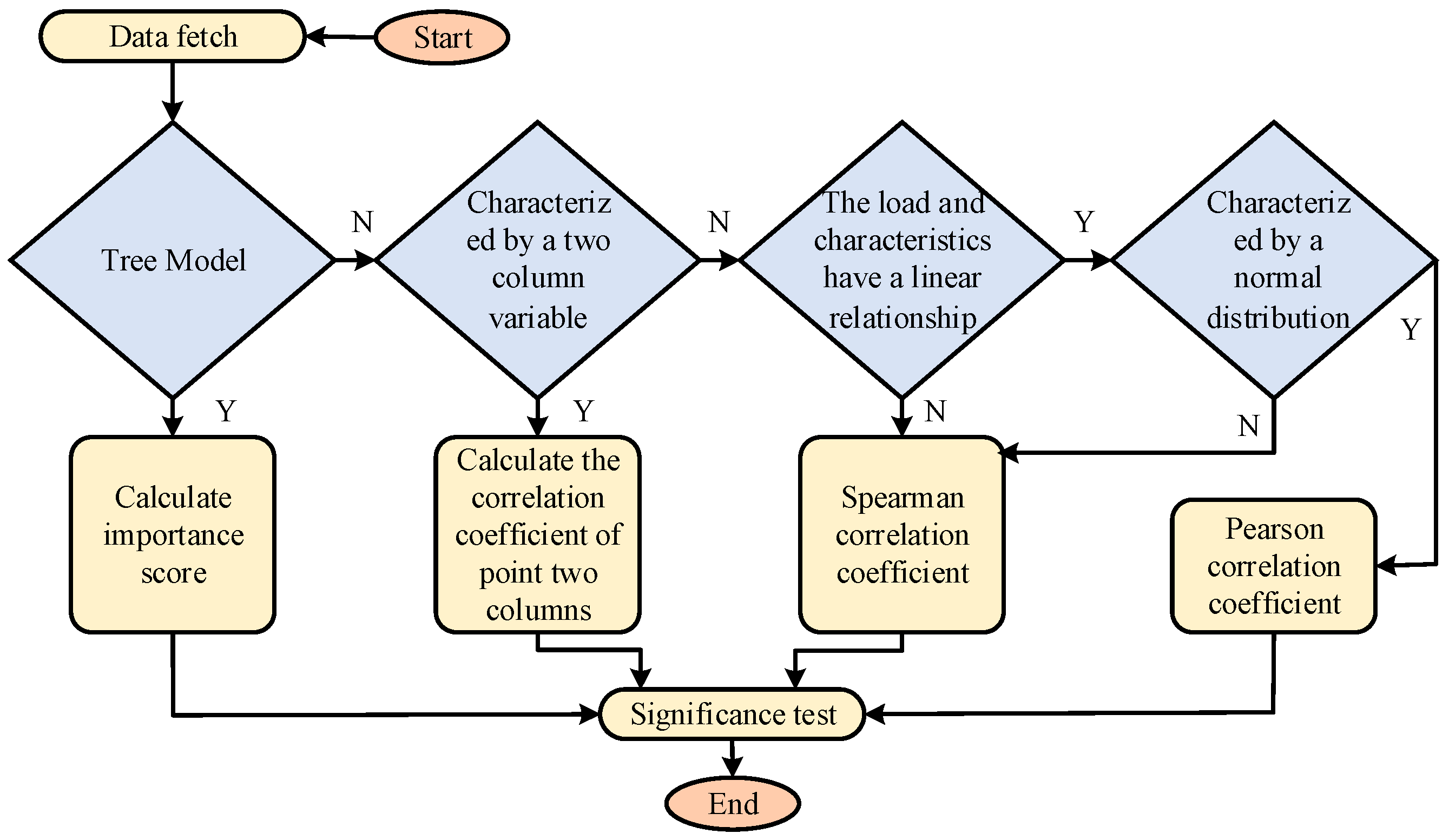
In Equation (1), $P_{d,t}^{\left(i\right)}$ represents the load of the $i$-th enterprise at time $t$ on day $d$, and the unit is kW; $n$ represents the number of levels. It can measure the correlation between power load and various features [21,22,23]. Different features require different correlation analysis methods, and the specific analysis process is shown in Figure 3.

In Figure 3, the Pearson correlation coefficient is applicable to continuous variables with a linear relationship and data following a normal distribution [24,25,26], as shown in Equation (2).

$${\rho }_{X,Y}={\displaystyle \frac{COV\left(X,Y\right)}{\sqrt{D\left(X\right)D\left(Y\right)}}}={\displaystyle \frac{E\left[\left(X-{\mu }_X\right)\left(Y-{\mu }_Y\right)\right]}{\sqrt{D\left(X\right)D\left(Y\right)}}},$$

(2)

In Equation (2), $COV\left(X,Y\right)$ represents covariance, $D$ represents variance, and $\mu$ represents the mean. The Spearman rank correlation coefficient is applicable to variables with curved relationships or non-normal distributions [27,28]. Equation (3) illustrates Spearman’s calculation method.

$${\rho }_{X,Y}=1-{\displaystyle \frac{6\sum d_i^2}{n^3-n}},$$

(3)

In Equation (3), $d$ represents the level difference between paired variables in two columns. The point two column correlation coefficient is used to measure the correlation between continuous variables and binary variables, as shown in Equation (4).

$$R={\displaystyle \frac{{\overline{X}}_p-{\overline{X}}_q}{\sigma }}\times \sqrt{pq},$$

(4)

In Equation (4), $p$ and $q$ are the frequency ratios of binary variables, $R$ indicates the correlation between continuous and dichotomous variables, and ${\overline{X}}_p$ and ${\overline{X}}_q$ are the mean values of continuous variables. Noise processing can be divided into data skewing processing and systematic denoising [29,30,31,32]. Data skewing processing can be divided into inter-class data imbalance, intra-class positive and negative sample imbalance, and data distribution imbalance in the sample space. For the first category, the Kullback–Leible divergence balance adjustment algorithm is adopted. The second type is solved by optimizing data distribution, adjusting normalization strategies, and removing outlier data. The third type involves the use of normality fitting tests and processing through methods such as re-partitioning the dataset and removing outliers. Systematic noise reduction mainly deals with the noise caused by multiple factors and independent factors of power load. Due to the interference between complex cross-domain data, effective denoising becomes difficult. Therefore, distinguishing between similar and dissimilar data has become an important aspect of denoising. This study proposes a novel denoising method that fully utilizes load characteristics and curve shape features by re-partitioning the dataset, aggregating similar information, and stripping out dissimilar information to achieve denoising.

This study divides the data domain for denoising into four steps. Step 1: The data are divided according to administrative regions to reduce cross-regional interference. Step 2: The data are divided according to industry data and the influence of industry rules is eliminated. Step 3: The data are divided into clusters based on load characteristics, collecting the load characteristics of electricity users and aggregating enterprises with similar characteristics. However, the above three parts cannot solve factors unrelated to load characteristics and increase uncertainty. Therefore, in the fourth step, this study uses Fourier transform to extract the main features of enterprises and cluster them to eliminate interference between curve shapes. When dividing based on load feature clustering, it is necessary to calculate the load features of the enterprise, and the coefficient of variation is shown in Equation (5).

$$y_v=y_{std}\sqrt{y},$$

(5)

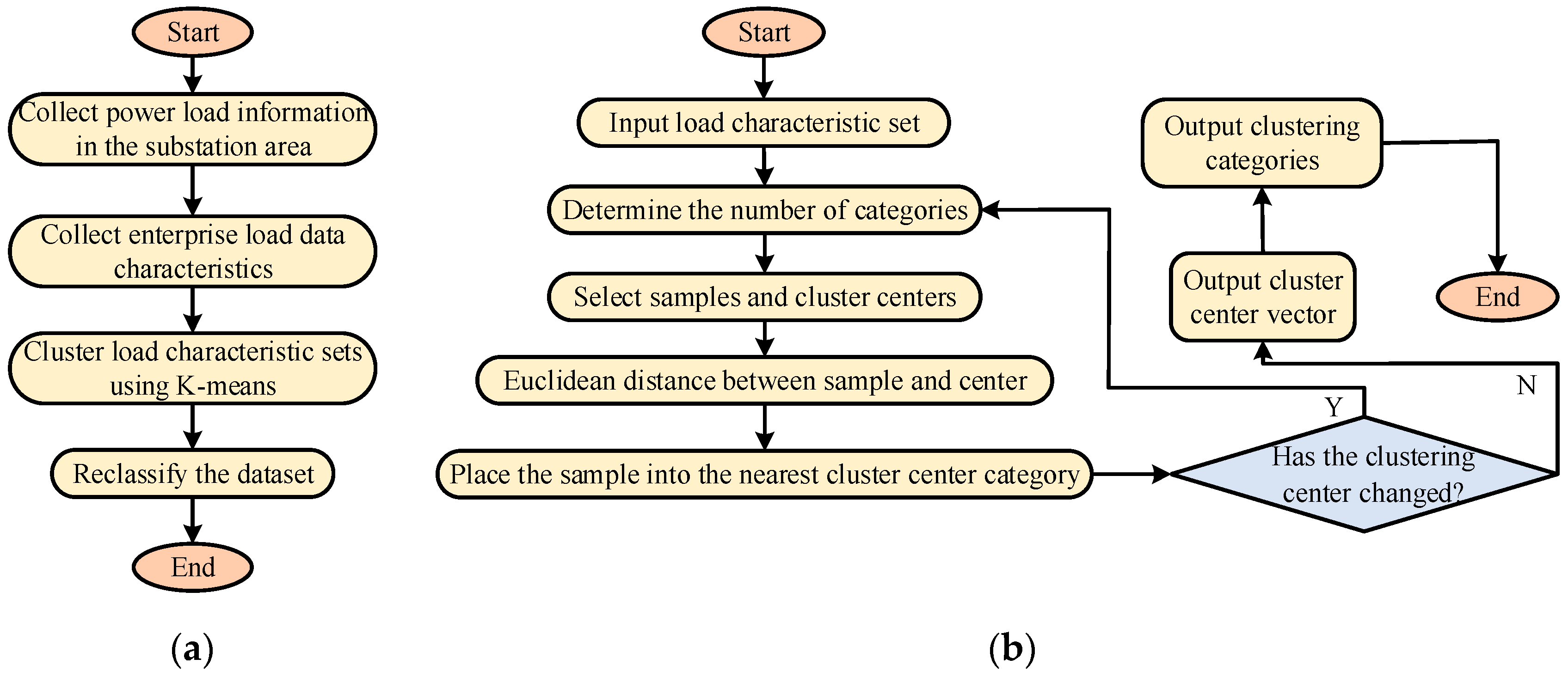
In Equation (5), $y$ represents the eigenvector, and $std\sqrt{y}$ represents the standard deviation. The flow and operation steps of the load characteristic clustering algorithm are shown in Figure 4.

In Figure 4, clustering is the process of repeating iterations until the center stabilizes or reaches the largest iteration, and the dataset is redivided after classification is completed. In the fourth step, this study extracts periodic components through Fourier transform and decomposes the power load, as shown in Equation (6).

$$P\left(t\right)=a_0+D\left(t\right)+W\left(t\right)+L\left(t\right)+H\left(t\right),$$

(6)

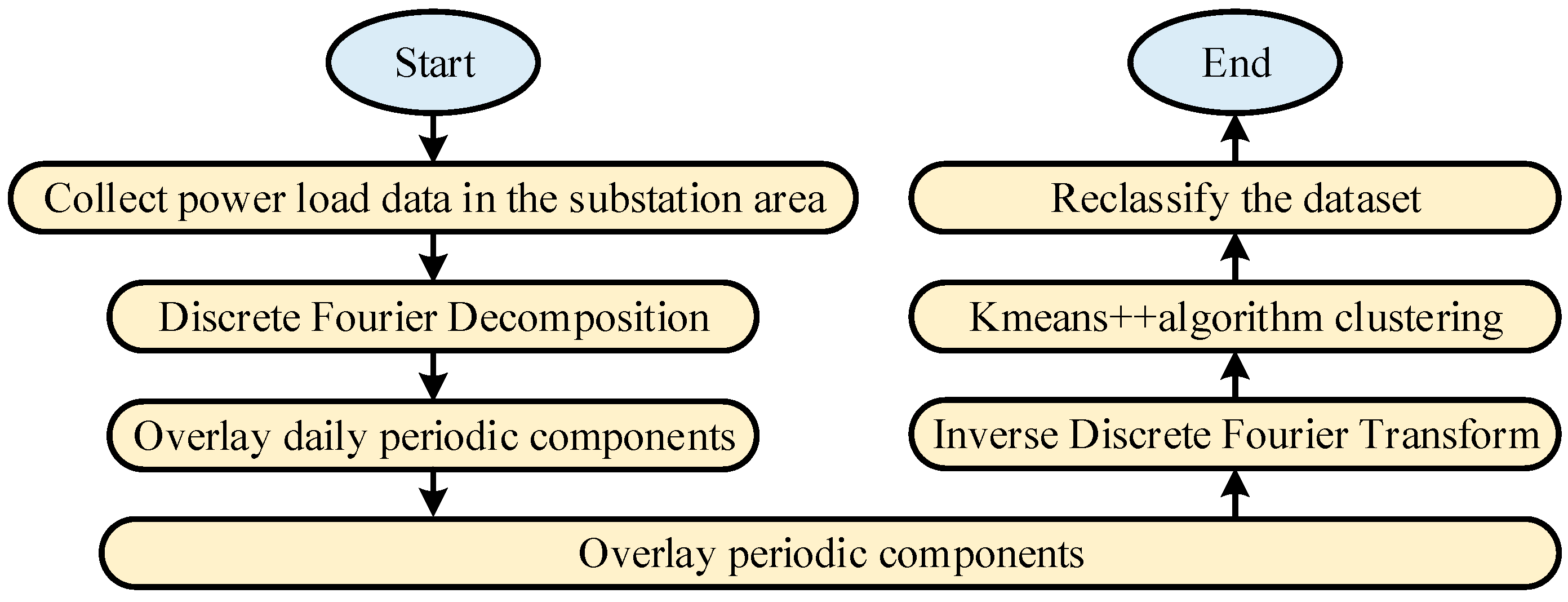
In Equation (6), the period can be decomposed into the daily period component $D\left(t\right)$, weekly period component $W\left(t\right)$, mid-low frequency component $L\left(t\right)$, and high-frequency noise $H\left(t\right)$. In the selection of frequency-domain decomposition algorithms, considering the special requirements of load data clustering, this study chose the discrete Fourier transform method. This method can preserve the main periodic features of data and effectively extract the frequency spectrum of daily and weekly cycles, with strong interpretability and adaptability. The denoising algorithm process is shown in Figure 5.

In Figure 5, firstly, the power load data of each electricity-consuming enterprise are represented as a time-domain sequence, and the power load sequence is shown in Equation (7).

$$D_i^{\prime }=\left(S_0^{\left(i\right)},S_0^{\left(i\right)},\dots ,S_n^{\left(i\right)},\dots ,S_{N-1}^{\left(i\right)}\right),$$

(7)

In Equation (7), $S_n^{\left(i\right)}$ represents the load value, $i$ represents the enterprise serial number, and $n$ represents the time. Then, the time-domain signal is converted into a frequency-domain signal, and the amplitude of each enterprise load data at different frequencies is calculated, as shown in Equation (8).

$$F^{\left(i\right)}\left({\omega }_k\right)={\sum }_{n=0}^{N-1}{S}_n^{\left(i\right)}{e}^{-j\left({\displaystyle \frac{2\pi }{N}}\right)nk},$$

(8)

In Equation (8), ${\omega }_k$ represents angular frequency, and $k$ represents the periodic index. Based on the frequency-domain signal, the daily and weekly components of the power load data are extracted. The daily component corresponds to the repetitive characteristics of the load data every day, while the weekly component reflects the weekly load change pattern. In order to enhance the reliability of the signal, the daily and weekly components are superimposed together to form a denoised frequency-domain signal. The superimposed frequency-domain signal not only retains the main features of the original load data but also filters out some high-frequency noise and enhances data stability. The superimposed signal is shown in Equation (9).

$${\tilde{F}}^{\left(i\right)}\left({\omega }_k\right)=I\left[k\in \left(E_{Day}\cup E_{Weak}\right)\right]F^{\left(i\right)}\left({\omega }_k\right),$$

(9)

In Equation (9), $E_{Day}$ represents the daily period component, and $E_{Weak}$ represents the weekly period component. After frequency-domain processing is completed, it is restored to the time-domain signal, and the original appearance of the processed time series is preserved, as shown in Equation (10).

$$S_n^{\left(i\right)}={\displaystyle \frac{1}{N}}{\sum }_{k=0}^{N-1}{e}^{j\left({\displaystyle \frac{2\pi }{N}}\right)nk}{\tilde{F}}^{\left(i\right)}\left({\omega }_k\right),$$

(10)

Finally, in the clustering process, to better measure the similarity between different enterprises, dynamic time planning distance is adopted as the similarity measurement standard of Kmeans++ to align time series more flexibly, adapt to the comparison between sequences of different lengths and shapes, and ensure clustering accuracy.

2.2. Adversarial Adaptive LF Model

Data processing and noise reduction techniques have laid the data foundation for LF. By reducing noise and outliers in the data, the forecasting model can be made to more accurately capture the changing patterns of power loads, thus improving the accuracy and reliability of forecasts. The next step is to design the forecasting model. The domain-shift problem often occurs in LF. This study designs a Transformer LF model with an adversarial adaptive mechanism. Domain partitioning is a crucial step. Appropriate domain partitioning methods can effectively identify domain-shift phenomena, thereby improving the adaptability. This study uses a designed four-step method for domain partitioning and introduces the Maximum Mean Difference (MMD) algorithm to calculate the mean difference in data mapping. The loss of maximizing the mean difference is shown in Equation (11).

$$MMD\left(x_i,y_i\right)={‖{\displaystyle \frac{1}{n}}{\sum }_{i=1}^n\Phi \left(x_i\right)-{\displaystyle \frac{1}{m}}{\sum }_{i=1}^n\Phi \left(y_i\right)‖}^2=tr\left(KL\right),$$

(11)

In Equation (11), $x_i$ and $y_i$ represent independent samples; $i=\mathrm{1,2},\dots ,n$, $j=\mathrm{1,2},\dots ,m$. The adversarial adaptive machine is the core mechanism of the model, which is based on generative adversarial networks, and a feature extractor is used to align the feature space and reduce the impact of domain offset on model prediction accuracy through the adversarial training mechanism. The domain discriminator, as a data source judgment tool, has optimization objectives as shown in Equation (12).

$$O=\underset{{\theta }_D}{\min } \underset{{\theta }_F}{\max } loss\left(Domain,Target\right),$$

(12)

In Equation (12), ${\theta }_F$ is the parameters of the feature extractor, and ${\theta }_D$ is the parameters of the domain discriminator. The architecture of the designed power load sequence prediction model is shown in Figure 6.

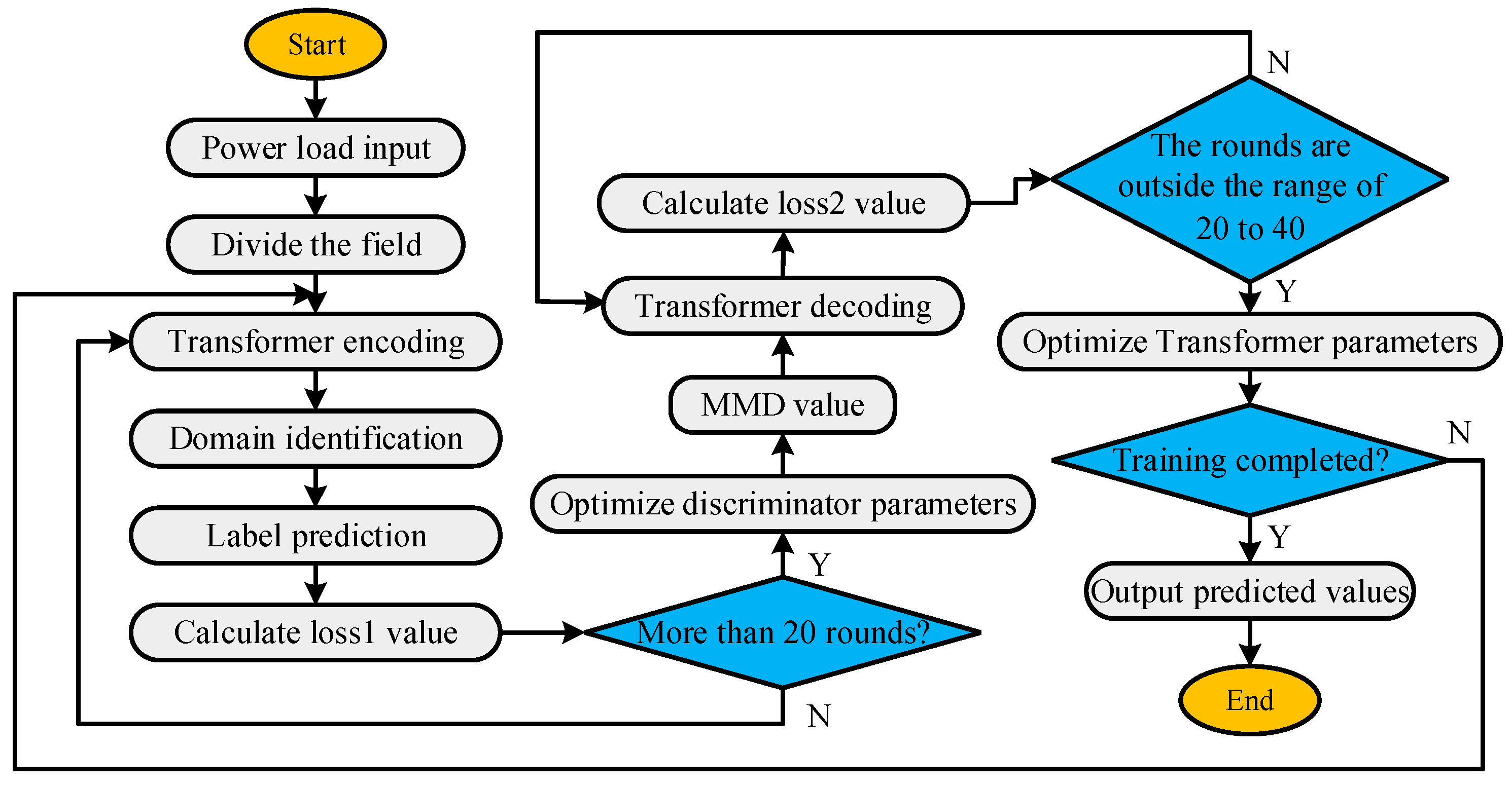
In Figure 6, the model can be divided into encoders, decoders, discriminators, etc. The encoder is responsible for extracting dense information from power loads. It enhances the ability to extract temporal features by introducing position information encoders and temporal mask units, and captures local features of power loads through operations such as translation, distortion, and scaling invariance of convolution kernels. The decoder uses long short-term networks and multi-layer perceptrons to process these features. By calculating the correlation information between different locations multiple times, it obtains more significant representations of power load characteristics and generates load prediction values. The intermediate domain discriminator is applied to distinguish whether the input features come from the source domain or the target domain. The algorithm flow of the adaptive Transformer is shown in Figure 7.

In Figure 7, the training process of the adaptive Transformer is divided into a pre-training stage and an adversarial adaptive training stage. In the pre-training phase, the parameters of the domain discriminator are frozen, and independent training of the encoder and decoder is first performed to ensure that the encoder can output meaningful feature representations. In the adversarial adaptive training phase, the encoder, decoder, and domain discriminator are alternately trained. The discriminator minimizes domain label prediction, with cross-entropy loss as shown in Equation (13).

$${loss}_1=-{\displaystyle \frac{1}{n}}{\sum }_{i=1}^{n}l\widehat{\mathit{log}l}+(1-l)\mathit{log}(1-\widehat{l}),$$

(13)

In Equation (13), $l$ represents the true domain label, and $\widehat{l}$ represents the predicted domain label. Then, the encoder and decoder are co-trained. Domain-invariant information is generated while minimizing the mean square error (MSE) of load prediction. The co-trained loss function is shown in Equation (14).

$${loss}_2=-los{s}_1-MMD\left(D,S\right)+MSE\left(\widehat{y},y\right),$$

(14)

In Equation (14), $MMD\left(D,S\right)$ represents the MMD value and $MSE\left(\widehat{y},y\right)$ represents the MSE. After training, the model can output accurate power load prediction values and achieve distribution alignment between the source domain and the target domain, thereby addressing domain-shift issues and improving prediction accuracy.

3. Results

This study analyzed the denoising clustering effect and LF effect separately. When analyzing the denoising clustering effect, different data partitioning methods were compared and parameter tuning analysis was conducted. When analyzing the effectiveness of LF, it was divided into real-time, short-term, and long-term LF, and the model performance was compared horizontally. The ablation test was used to verify the superiority of the improved model.

3.1. Analysis of Denoising Clustering Effect

Before analyzing the effectiveness of LF, data processing clustering methods were analyzed to test the partitioning effect on the dataset during data processing. The results of clustering parameter adjustment are shown in Figure 8.

In Figure 8a, the relationship between initialization times and contour coefficients is not clear. In Figure 8b, the relationship between the maximum number of iterations and the contour coefficient is also not clear. In Figure 8c, when the number of clusters is above 35 and the contour coefficient reaches below 0.5, the clustering effect decreases significantly. In Figure 8d, when the clusters increase, the number of classified invalid enterprises shows an increasing trend. When the clusters are below 35, the number of classified invalid enterprises is below 80, which is more appropriate. The MSE comparison of the partition methods is shown in Table 1.

In Table 1, the comparison of mean values provided valuable information. The MSE by the industry division method was 0.160, slightly higher than the MSE by region division, which was 0.156. The MSE of Fourier transform clustering was 0.154, which was the lowest overall. The MSE of load characteristic clustering was the highest, at 0.170, indicating that it was relatively weak in overall performance, while the Fourier transform clustering designed in the research focus performed the best. Meanwhile, Fourier transform clustering was more suitable for unsupervised domain adaptation problems and had stronger applicability than other methods.

3.2. Analysis of LF Effectiveness

The comparison algorithms used in the study include Dynamic Time Warping–Long Short-Term Memory (DTW-LSTM), Support Vector Regression (SVR), Classification and Regression Tree (CART), eXtreme Gradient Boosting (XGB), Gradient Boosting Decision Tree (LGB), Logistic Regression (LR), Gradient Boosting Decision Tree (GBDT), Logistic Regression (LR), random forest (RF), Light Gradient Boosting Machine (LGBM), Convolutional Neural Network–Long Short-Term Memory (CNN-LSTM), and Transformer. The analysis of LF effectiveness was divided into three aspects: real-time load, short-term load, and long-term load. The specific results are illustrated in Figure 9.

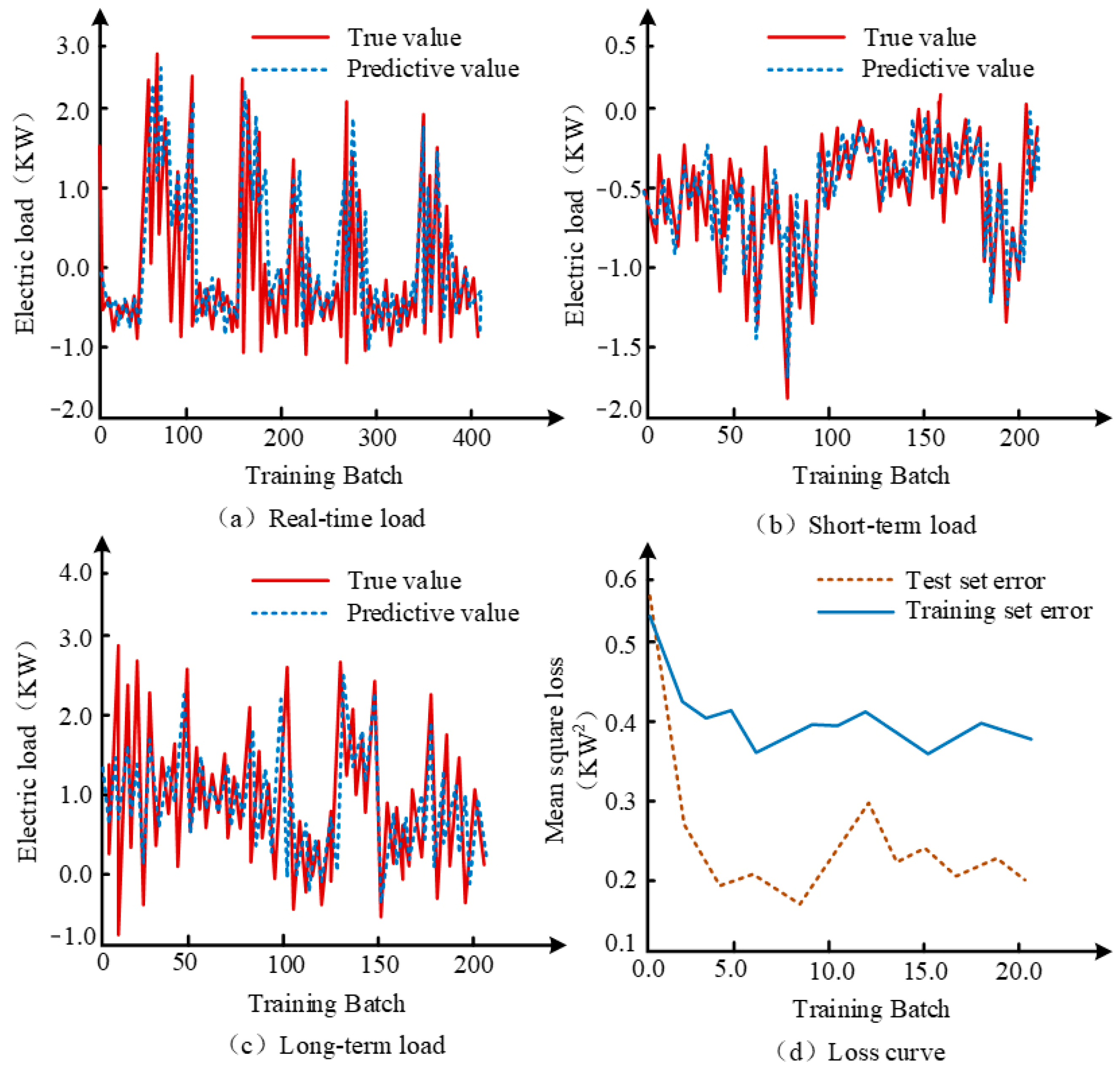
In Figure 9, the research model exhibits different information-fitting characteristics. In Figure 9a, the real-time load exhibits significant step and periodicity, and the research model has a strong capture ability for this periodicity and can track the curve well. In Figure 9b, the randomness of short-term loads is strong, and the research model has a high degree of fit to this nonlinear characteristic. In Figure 9c, the long-term load exhibits high volatility, and the research model has strong tracking ability for the high-frequency part. In Figure 9d, the loss curve of the training set is relatively higher, while the loss curve of the testing set is lower. Therefore, the research model had better performance in practical applications.

Table 2. Ablation test.

Dataset	Research Model	Adversarial Adaptive Module	MMD Module	Adversarial Adaptation and MMD Module	Attention Is Placed on the Encoder	Attention Is Placed on the Decoder
Collection 1	0.269	0.284	0.270	0.277	0.217	0.154
Collection 2	0.260	0.263	0.261	0.265	0.260	0.210
Collection 3	0.178	0.183	0.185	0.206	0.186	0.169
Collection 4	0.375	0.390	0.379	0.418	0.390	0.189
Collection 5	0.158	0.159	0.156	0.163	0.155	0.151
Collection 6	0.143	0.148	0.145	0.149	0.132	0.125
Collection 7	0.357	0.372	0.362	0.397	0.271	0.150
Collection 8	0.439	0.458	0.439	0.453	0.330	0.262
Collection 9	0.284	0.307	0.303	0.320	0.177	0.170
Average value	0.274	0.285	0.278	0.293	0.236	0.176

illustrates the results of the ablation test.

In Table 2, the adversarial adaptive module, the MMD module, and the adversarial adaptive and MMD modules were separately removed from the research model and compared. From the comparison results, in the first four columns of data, the MSE of the research model was 0.274. After revoking the adversarial adaptive module, the MSE was 0.285. After revoking the MMD module, the MSE was 0.278. After revoking the adversarial adaptation and MMD module, the MSE was 0.293. The research model had the lowest MSE value in its complete form, indicating that the adversarial adaptive method proposed in this study could maintain optimal performance. The MSE of the attention module placed in the encoder part was 0.236 and the MSE of the attention module placed in the decoder part was 0.176, which showed that the model performed better when the Attention module was placed in the decoder part. The error analysis of three types of LF analysis is shown in

Table 3. Analysis of three types of LF errors.

Load Type	Dataset	DTW-LSTM	SVR	CART	XGB	LGB	Research Model
Long-term load	Collection 1	0.020	0.040	0.062	0.052	0.058	0.010
	Collection 2	0.008	0.038	0.038	0.045	0.035	0.026
	Collection 3	0.105	0.101	0.031	0.117	0.050	0.043
	Collection 4	0.090	0.092	0.013	0.060	0.074	0.026
	Collection 5	0.079	0.071	0.133	0.177	0.346	0.162
	Average value	0.060	0.068	0.055	0.090	0.113	0.053
Short-term load	Collection 1	0.018	0.045	0.058	0.049	0.056	0.012
	Collection 2	0.016	0.032	0.035	0.046	0.034	0.027
	Collection 3	0.103	0.096	0.029	0.107	0.056	0.041
	Collection 4	0.095	0.083	0.014	0.062	0.268	0.025
	Collection 5	0.064	0.068	0.115	0.169	0.341	0.157
	average value	0.059	0.065	0.050	0.087	0.151	0.052
Real-time load	Collection 1	0.028	0.022	0.024	0.026	0.006	0.016
	Collection 2	0.085	0.085	0.055	0.086	0.104	0.009
	Collection 3	0.707	3.527	1.296	0.801	0.552	0.688
	Collection 4	0.251	0.493	0.361	0.306	0.286	0.261
	Collection 5	0.082	0.117	0.157	0.098	0.209	0.101
	Average value	0.231	0.849	0.378	0.263	0.231	0.215

.

In Table 3, the MSE of the research model for long-term LF is 0.053; the MSEs of SVR, CART, XGB, LGB, and DTW-LSTM are 0.068, 0.055, 0.090, 0.113, and 0.060. In long-term LF, the MSE value of the research model was the lowest and the prediction was the most accurate. In short-term LF, the MSE of the research model was 0.052. The MSEs of SVR, CART, XGB, LGB, and DTW-LSTM were 0.065, 0.055, 0.087, 0.151, and 0.059, respectively, all higher than the research model. Therefore, the research model had an accuracy advantage in short-term LF. In real-time LF, the MSE of the research model was 0.215. The MSEs of SVR, CART, XGB, LGB, and DTW-LSTM were 0.849, 0.378, 0.263, 0.231, and 0.231, respectively. Therefore, in real-time LF, the research model had the best LF effect and the most accurate results. Overall, the research model had the highest prediction accuracy in long-term, short-term, and real-time LF. The model training loss curve is shown in Figure 10.

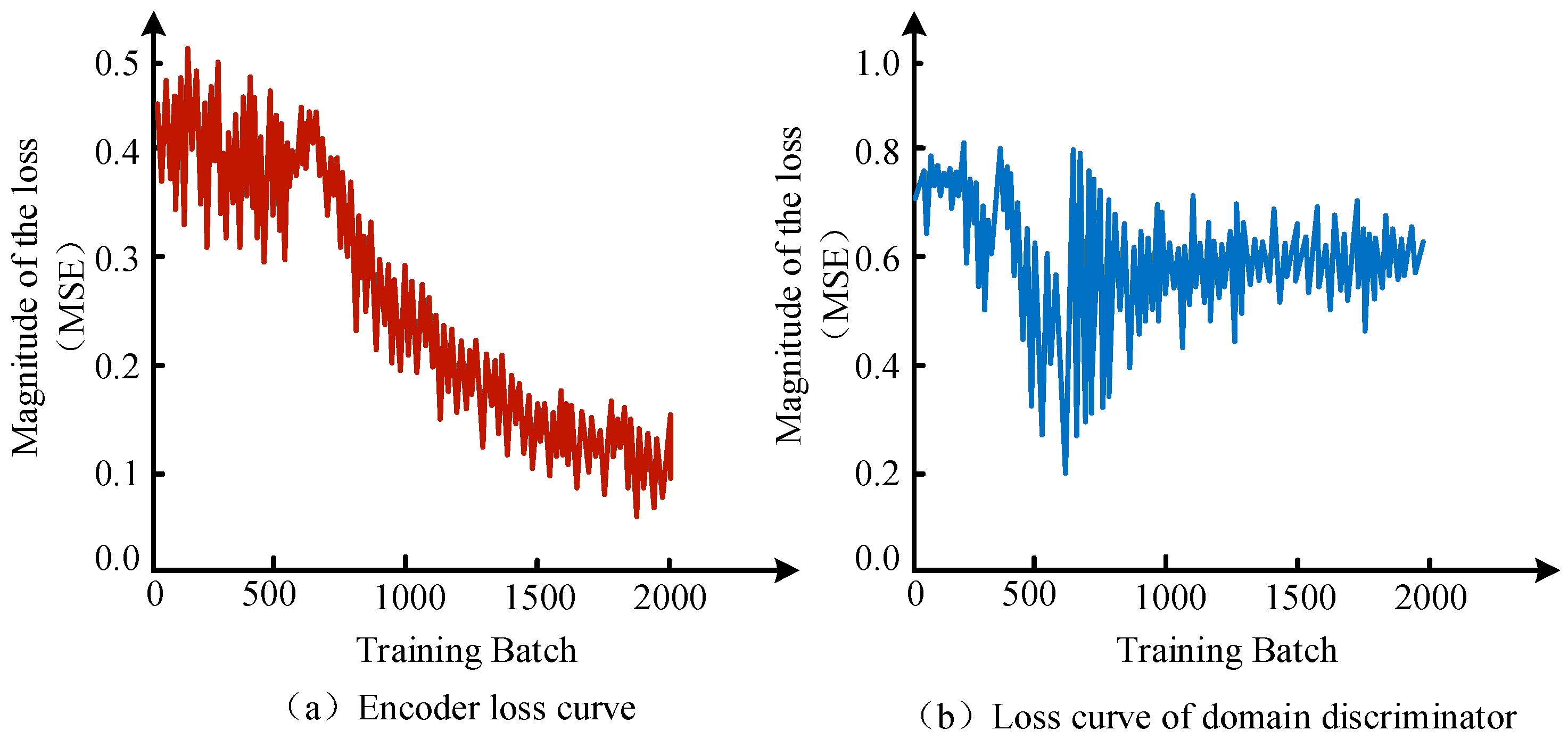
In Figure 10a, during the training phase, the loss curve shows a slight increase in the early stage and a rapid decrease in the later stage, which is due to the fixed explanation of the encoder and decoder. In Figure 10b, during the training phase, the curve oscillates strongly. This is because during the training phase, the encoder output domain-invariant information to reduce discrimination loss. The LF loss curve is shown in Figure 11.

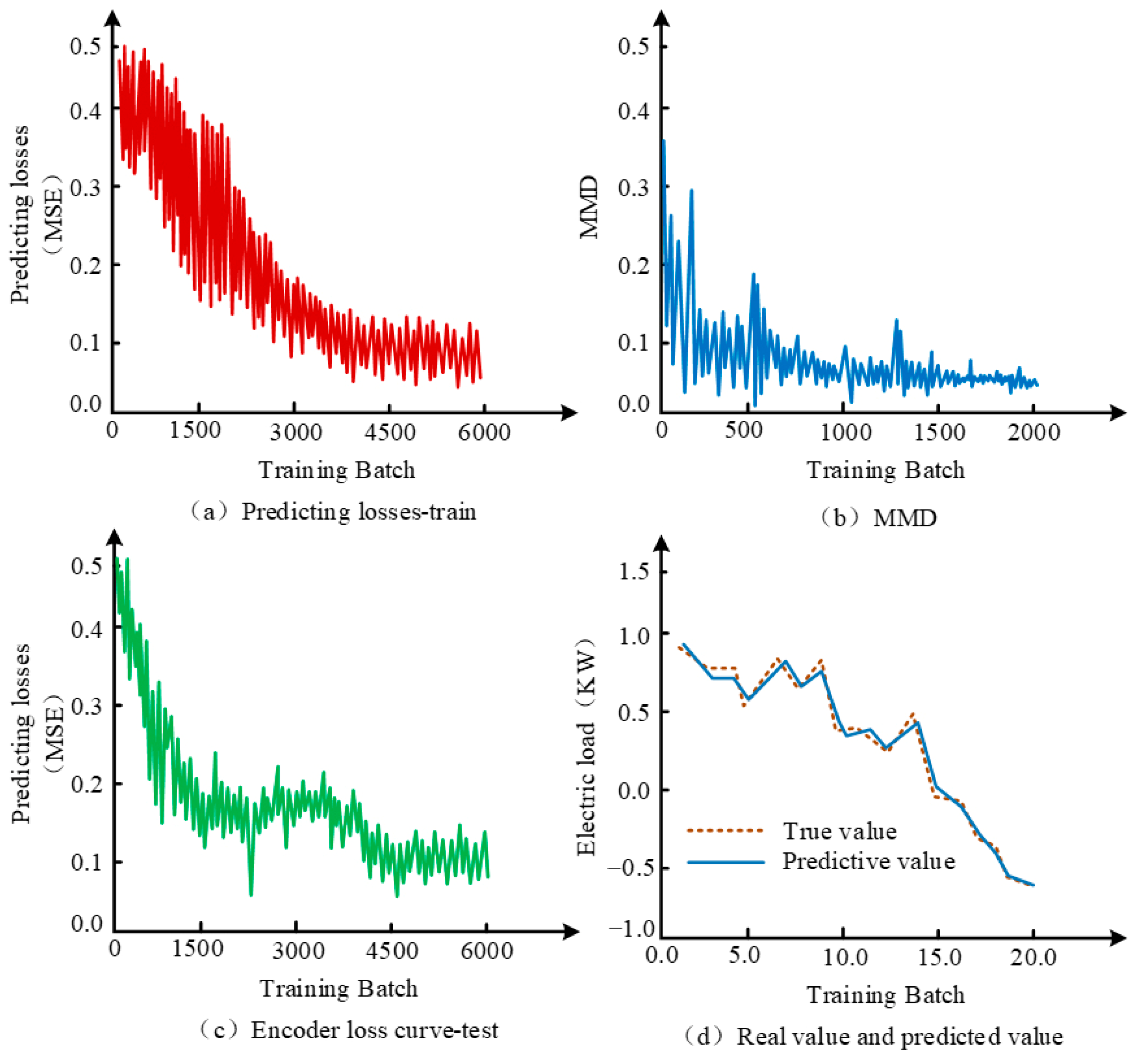
In Figure 11a, the loss curve during the training phase shows a stable downward trend and reaches convergence after about 4500 iterations. In Figure 11c, the loss curve of the model also shows a monotonic downward trend during the testing process and reaches convergence after about 4500 iterations. In Figure 11b, the MMD curve shows a trend of gradually decreasing fluctuation, which is because the output results of the encoder with a large size could be trained for a certain number of rounds after projection to reduce the MMD and achieve distribution alignment. In Figure 11d, there is a relatively consistent trend between the true values and the predicted values. Therefore, the research model had strong predictive ability. The different ranges of the horizontal axis are due to the different number of training steps and iterations required for the model’s MMD module. The horizontal performance comparison of the models is shown in

Table 4. Comparison of model lateral performance.

Dataset (MMD)	MMD = 0.45	MMD = 0.25	MMD = 0.18	MMD = 0.07	MMD = 0.02	MMD = 0.01	MMD = 0.00	Average Value
Research model	0.076	0.120	0.089	0.119	0.149	0.114	0.136	0.113
XGB	0.186	0.147	0.235	0.148	0.26	0.203	0.204	0.221
SVR	0.332	0.190	0.343	0.249	0.565	0.427	0.251	0.321
LR	0.331	0.178	0.279	0.258	0.495	0.386	0.249	0.288
RF	0.331	0.151	0.264	0.245	0.444	0.377	0.229	0.286
LGBM	0.211	0.137	0.199	0.100	0.312	0.204	0.228	0.215
CART	0.385	0.172	0.349	0.326	0.527	0.433	0.233	0.333
DTW-LSTM	0.091	0.137	0.098	0.192	0.192	0.053	0.193	0.127
CNN-LSTM	0.093	0.133	0.116	0.076	0.129	0.095	0.168	0.129
Transformer	0.092	0.168	0.258	0.181	0.122	0.114	0.171	0.15

.

In Table 4, the research model demonstrates significant advantages. In the case of MMD = 0.45, the MSE of the research model was 0.076, which was significantly lower than other models. This indicated that in the case of large differences in data distribution, the research model could better adapt to complex data distribution situations, reduce prediction errors, and improve prediction accuracy. At MMD = 0.25, the MSE of the research model was 0.120, which was lower than other models. At MMD = 0.19, the MSE of the research model was 0.089, which was also lower than other models. Overall, when the MMD value was less than 0.18, the MSE of the research model was also relatively low. From this, the research model had a strong domain adaptation ability. When cross-domain phenomena occurred in the data, this accuracy could still be stably displayed, demonstrating the stability of the model. The research model had significant advantages when dealing with complex and diverse datasets. Overall, in the case of imbalanced intra-class data and significant distribution differences in data from different regions or time periods, the research model could ensure good predictive performance when processing minority class data, and had better generalization ability between different data domains, which could adapt to the LF needs of different regions or time periods. This study contributes to the development of intelligent control power systems. Through precise LF, power companies can more accurately schedule and allocate power resources, improve the overall operational efficiency of the power system, and reduce energy waste. This study tested the performance of the model based on real historical electricity data from different cities. Among them, two were Digital 1 and Digital 2 for coastal cities, one was Digital 3 for inland cities with sufficient new energy generation capacity, and one was Digital 4 for inland cities with sufficient hydroelectricity generation capacity, and the relevant data were downloaded from the local online platform of the State Grid. The results are shown in

Table 5. Performance comparison of real data in different regions of model testing.

	Data Sources	Research Model	CNN-LSTM	CNN-GRU
Predictive accuracy	Digital 1	98.4%	93.5%	95.2%
	Digital 2	97.6%	91.4%	93.1%
	Digital 3	93.5%	89.6%	90.4%
	Digital 4	98.1%	95.3%	96.5%

.

As shown in Table 5, this study proposes that the predictive accuracy of the model is higher than both deep learning algorithms, with the model’s predictive accuracy being 4.9% and 3.2% higher than that of CNN-LSTM and CNN-GRU, respectively, in Digital 1. The largest gap in prediction accuracy was in Digital 2, where the model’s prediction accuracy was 6.2% and 4.5% higher than the two algorithms.

4. Discussion and Conclusions

To solve the problems of data imbalance and inaccurate prediction in power LF, this study designed a Transformer LF model that combines an adversarial adaptive mechanism with data denoising technology to cope with domain-shift phenomena in the dataset and make more accurate predictions. The MSE of the Fourier transform clustering used in this study was 0.154, indicating better data partitioning performance. The MSEs in the prediction of long-term load, short-term load, and real-time load were 0.053, 0.052, and 0.215, respectively. The loss curves of the model converged after about 4500 iterations during both the training and testing phases. In addition, the true value curve of power load showed a relatively consistent trend with the predicted value of power load, indicating that the research model had strong predictive ability. In horizontal comparison, under domain offset, when the MMD value was 0.45, the MSE of the research model was 0.076. When the MMD values were 0.25 and 0.19, the MSE of the research model was 0.120 and 0.089. As a result, the model designed in this study can effectively deal with the phenomenon of domain offset, improve the accuracy and precision of power load prediction, have high stability in practical application, effectively improve the overall operating efficiency of the power system, and reduce the waste of resources. Although the method designed by this study has better applicability, it is only aimed at predicting large electricity loads in a conventional urban electricity environment. Moreover, it does not analyze other special electricity environments, so the modular improvement of the model based on other special electricity environments is the direction of future research.

References

1. Farrag, T.A.; Elattar, E.E. Optimized deep stacked long short-term memory network for long-term load forecasting. IEEE Access 2021, 9, 68511–68522. [Google Scholar] [CrossRef]
2. Chiu, M.C.; Hsu, H.W.; Chen, K.S.; Wen, C.Y. A hybrid CNN-GRU based probabilistic model for load forecasting from individual household to commercial building. Energy Rep. 2023, 9, 94–105. [Google Scholar] [CrossRef]
3. Mubashar, R.; Awan, M.J.; Ahsan, M.; Yasin, A.; Singh, V.P. Efficient residential load forecasting using deep learning approach. Int. J. Comput. Appl. Technol. 2022, 68, 205–214. [Google Scholar] [CrossRef]
4. Van den Ende, M.; Lior, I.; Ampuero, J.P.; Sladen, A.; Ferrari, A.; Richard, C. A self-supervised deep learning approach for blind denoising and waveform coherence enhancement in distributed acoustic sensing data. IEEE Trans. Neural Netw. Learn. Syst. 2021, 34, 3371–3384. [Google Scholar] [CrossRef]
5. Li, Q.; Li, Q.; Han, Y. A Numerical Investigation on Kick Control with the Displacement Kill Method during a Well Test in a Deep-Water Gas Reservoir: A Case Study. Processes 2024, 12, 2090. [Google Scholar] [CrossRef]
6. Xu, P.; Shin, I. Preparation and Performance Analysis of Thin-Film Artificial Intelligence Transistors Based on Integration of Storage and Computing. IEEE Access 2024, 12, 30593–30603. [Google Scholar] [CrossRef]
7. Li, J.; Wei, S.; Dai, W. Combination of manifold learning and deep learning algorithms for mid-term electrical load forecasting. IEEE Trans. Neural Netw. Learn. Syst. 2021, 34, 2584–2593. [Google Scholar] [CrossRef]
8. Ozer, I.; Efe, S.B.; Ozbay, H. A combined deep learning application for short term load forecasting. Alex. Eng. J. 2021, 60, 3807–3818. [Google Scholar] [CrossRef]
9. Liu, Y.; Dutta, S.; Kong, A.W.K.; Yeo, C.K. An image inpainting approach to short-term load forecasting. IEEE Trans. Power Syst. 2022, 38, 177–187. [Google Scholar] [CrossRef]
10. Zhu, Y.Q.; Cai, Y.M.; Zhang, F. Motion capture data denoising based on LSTNet autoencoder. J. Internet Technol. 2022, 23, 11–20. [Google Scholar] [CrossRef]
11. Li, X.; Feng, S.; Hou, N.; Wang, R.; Li, H.; Gao, M.; Li, S. Surface microseismic data denoising based on sparse autoencoder and Kalman filter. Syst. Sci. Control Eng. 2022, 10, 616–628. [Google Scholar] [CrossRef]
12. Feng, J.; Li, X.; Liu, X.; Chen, C.; Chen, H. Seismic data denoising based on tensor decomposition with total variation. IEEE Geosci. Remote Sens. Lett. 2021, 18, 1303–1307. [Google Scholar] [CrossRef]
13. Tibi, R.; Hammond, P.; Brogan, R.; Young, C.J.; Koper, K. Deep learning denoising applied to regional distance seismic data in Utah. Bull. Seismol. Soc. Am. 2021, 111, 775–790. [Google Scholar] [CrossRef]
14. Dong, X.; Deng, S.; Wang, D. A short-term power load forecasting method based on k-means and SVM. J. Ambient Intell. Humaniz. Comput. 2022, 13, 5253–5267. [Google Scholar] [CrossRef]
15. Veeramsetty, V.; Reddy, K.R.; Santhosh, M.; Mohnot, A. Short-term electric power load forecasting using random forest and gated recurrent unit. Electr. Eng. 2022, 104, 307–329. [Google Scholar] [CrossRef]
16. Lv, L.; Wu, Z.; Zhang, J.; Zhang, L.; Tan, Z.; Tian, Z. A VMD and LSTM based hybrid model of load forecasting for power grid security. IEEE Trans. Ind. Inform. 2021, 18, 6474–6482. [Google Scholar] [CrossRef]
17. Yuan, J.; Wang, L.; Qiu, Y.; Wang, J.; Zhang, H.; Liao, Y. Short-term electric load forecasting based on improved Extreme Learning Machine Model. Energy Rep. 2021, 7, 1563–1573. [Google Scholar] [CrossRef]
18. Maharana, K.; Mondal, S.; Nemade, B. A review: Data pre-processing and data augmentation techniques. Glob. Transit. Proc. 2022, 3, 91–99. [Google Scholar] [CrossRef]
19. Song, X.F.; Zhang, Y.; Gong, D.W.; Gao, X.Z. A fast hybrid feature selection based on correlation-guided clustering and particle swarm optimization for high-dimensional data. IEEE Trans. Cybern. 2021, 52, 9573–9586. [Google Scholar] [CrossRef]
20. Wang, S.; Celebi, M.E.; Zhang, Y.-D.; Yu, X.; Lu, S.; Yao, X.; Zhou, Q.; Miguel, M.-G.; Tian, Y.; Gorriz, J.M.; et al. Advances in data preprocessing for biomedical data fusion: An overview of the methods, challenges, and prospects. Inf. Fusion 2021, 76, 376–421. [Google Scholar] [CrossRef]
21. Mastoi, M.S.; Zhuang, S.; Munir, H.M.; Haris, M.; Hassan, M.; Usman, M.; Bukhari, S.S.H.; Ro, J.-S. An in-depth analysis of electric vehicle charging station infrastructure, policy implications, and future trends. Energy Rep. 2022, 8, 11504–11529. [Google Scholar] [CrossRef]
22. Verma, S.; Dwivedi, G.; Verma, P. Life cycle assessment of electric vehicles in comparison to combustion engine vehicles: A review. Mater. Today Proc. 2022, 49, 217–222. [Google Scholar] [CrossRef]
23. Elberry, A.M.; Thakur, J.; Santasalo-Aarnio, A.; Larmi, M. Large-scale compressed hydrogen storage as part of renewable electricity storage systems. Int. J. Hydrogen Energy 2021, 46, 15671–15690. [Google Scholar] [CrossRef]
24. Deng, J.; Deng, Y.; Cheong, K.H. Combining conflicting evidence based on Pearson correlation coefficient and weighted graph. Int. J. Intell. Syst. 2021, 36, 7443–7460. [Google Scholar] [CrossRef]
25. Dufera, A.G.; Liu, T.; Xu, J. Regression models of Pearson correlation coefficient. Stat. Theory Relat. Fields 2023, 7, 97–106. [Google Scholar] [CrossRef]
26. Hidayanti, A.A.; Mandalika, E.N.D. The Pearson Correlation Analysis of Production Costs on the Land Area of Salt Farmers in Bolo Sub-District, Bima District. J. Inovasi Pendidik. Sains 2021, 2, 119–127. [Google Scholar] [CrossRef]
27. Amman, M.; Rashid, T.; Ali, A. Fermatean fuzzy multi-criteria decision-making based on Spearman rank correlation coefficient. Granul. Comput. 2023, 8, 2005–2019. [Google Scholar] [CrossRef]
28. Abd Al-Hameed, K.A. Spearman’s correlation coefficient in statistical analysis. Int. J. Nonlinear Anal. Appl. 2022, 13, 3249–3255. [Google Scholar]
29. Green, J.A. Too many zeros and/or highly skewed? A tutorial on modelling health behaviour as count data with Poisson and negative binomial regression. Health Psychol. Behav. Med. 2021, 9, 436–455. [Google Scholar] [CrossRef]
30. Xu, P.; Liu, H.; Zhang, H.; Lan, D.; Shin, I. Optimizing Performance of Recycled Aggregate Materials Using BP Neural Network Analysis: A Study on Permeability and Water Storage. Desalination Water Treat. 2024, 317, 100056. [Google Scholar] [CrossRef]
31. Ahmad, N.; Ghadi, Y.; Adnan, M.; Ali, M. Load forecasting techniques for power system: Research challenges and survey. IEEE Access. 2022, 10, 71054–71090. [Google Scholar] [CrossRef]
32. Geng, G.; He, Y.; Zhang, J.; Qin, T.; Yang, B. Short-term power load forecasting based on PSO-optimized VMD-TCN-attention mechanism. Energies 2023, 16, 4616. [Google Scholar] [CrossRef]
Figure 1. Structural anomalies.
Energies 17 05513 g001
Figure 2. Business anomalies.
Energies 17 05513 g002
Figure 3. Analysis of power load-related factors.
Energies 17 05513 g003
Figure 4. Flow of load characteristic clustering algorithm. (a) Load characteristic clustering algorithm. (b) Clustering algorithm process.
Energies 17 05513 g004
Figure 5. Noise reduction algorithm process.
Energies 17 05513 g005
Figure 6. Architecture of power load sequence prediction model.
Energies 17 05513 g006
Figure 7. Adaptive transformer algorithm process.
Energies 17 05513 g007
Figure 8. Cluster parameter adjustment results.
Energies 17 05513 g008
Figure 9. Real-time load, short-term load, and long-term LF effectiveness.
Energies 17 05513 g009
Figure 10. Model training loss curve.
Energies 17 05513 g010
Figure 11. LF loss curve.
Energies 17 05513 g011