Article

Aerodynamic Performance and Numerical Validation Study of a Scaled-Down and Full-Scale Wind Turbine Models

College of Civil Engineering and Architecture, Zhejiang University, Hangzhou 310058, China
*
Authors to whom correspondence should be addressed.
Energies 2024, 17(21), 5449; https://doi.org/10.3390/en17215449
Submission received: 7 September 2024 / Revised: 29 September 2024 / Accepted: 8 October 2024 / Published: 31 October 2024

Abstract

:
Understanding the aerodynamic performance of scaled-down models is vital for providing crucial insights into wind energy optimization. In this study, the aerodynamic performance of a scaled-down model (12%) was investigated. This validates the findings of the unsteady aerodynamic experiment (UAE) test sequence H. UAE tests provide information on the configuration and conditions of wind tunnel testing to measure the pressure coefficient distribution on the blade surface and the aerodynamic performance of the wind turbine. The computational simulations used shear stress transport and kinetic energy (SST K-Omega) and transitional shear stress transport (SST) turbulence models, with wind speeds ranging from 5 m/s to 25 m/s for the National Renewable Energy Laboratory (NREL) Phase VI and 4 m/s to 14 m/s for the 12% scaled-down model. The aerodynamic performance of both cases was assessed at representative wind speeds of 7 m/s for low, 10 m/s for medium, and 20 m/s for high flow speeds for NREL Phase VI and 7 m/s for low, 9 m/s medium, and 12 m/s for the scaled-down model. The results of the SST K-Omega and transitional SST models were aligned with experimental test measurement data at low wind speeds. However, the SST K-Omega torque values exhibited a slight deviation. The transitional SST and SST K-Omega models yielded aerodynamic properties that were comparable to those of the 12% scaled-down model. The torque values obtained from the simulation for the full-scale NREL Phase VI and the scaled-down model were 1686.5 Nm and 0.8349 Nm, respectively. Both turbulence models reliably predicted torque and pressure coefficient values that were consistent with the experimental data, considering specific flow regimes. The pressure coefficient was maximum at the leading edge of the wind turbine blade on the windward side and minimum on the leeward side. For the 12% scaled-down model, the flow simulation results bordering the low-pressure region of the blade varied slightly.

1. Introduction

Wind power generation has emerged as a primary, sustainable, and renewable power source and is gaining significant importance and economic viability in response to climate change and other power sources [1]. The design and optimization of wind turbine rotors remain challenging and significant owing to the complex wind flow environment [2,3]. The blades and hubs in wind turbines capture the force of the wind, and the captured wind force rotates the wind turbine rotor to convert the wind energy to electrical power. The design and performance of wind turbines rely heavily on the aerodynamic characteristics of the blades. Various research methodologies such as computational fluid dynamics (CFD), wind tunnel testing, the blade momentum method (BMM), and the vortex wake method have been employed in the field of aerodynamics [4]. Both eddy simulation (LES) and time-averaged Navier–Stokes equation (RANS) computational fluid dynamics (CFD) techniques have proven effective for studying wind turbine performance and analyzing the complex flows generated [5]. Recently, a high-fidelity optimization technique was also introduced to leverage the benefit of machine learning to reduce noise and improve aerodynamic efficiency. Geng et al. [6] proposed an advanced framework based on transfer learning and deep reinforcement learning to optimize the design. These methodologies helped to effectively optimize wind turbines to capture the maximum available energy.
In recent years, experimental research on the unsteady aerodynamic testing of the NREL wind turbine at NASA has been conducted at the Ames Wind Tunnel (80 × 120 feet) facility at the NREL, located in the United States of America. Later, researchers obtained simulation results using structural properties and geometries similar to those of the reference wind turbine provided by the NREL. The aerodynamic performance of NREL Phase VI was evaluated numerically using different models, such as the Navier–Stokes equations, wake-free, and blade element theory, under stall conditions for different yaw angle values. Their findings did not show a trend consistent with the experimental data, and a significant difference was observed between the predicted and actual observations [7,8,9]. Apart from the traditional CFD methods, to simulate complicated fluid dynamics, the lattice Boltzmann method (LBM) has gained popularity, especially in the case of wind turbine rotors. Lyu et al. [10] used advanced near-wall refinement to obtain better fluid flow predictions using a hybrid method in the LBM. This method has advanced the sliding mesh approach for LBM. Lyu et al. [11] applied the sliding method in the LBM as an alternative to traditional CFD approaches for wind turbine rotor simulation to capture complex flow dynamics.
Regardless of these differences, the above-mentioned numerical method provides a cost-effective and quick solution to differential equations by simulating fluid behaviors and wind turbine aerodynamic modeling. Several studies have used computational fluid dynamics (CFD) to investigate the aerodynamic characteristics of wind turbines. Menter et al. [12] presented two equation-based eddy viscosity turbulence models by incorporating the K-Omega and K-ε models near the inner and outer regions of boundary-layer walls. The transport of turbulent shear stress was incorporated into the formulation of turbulent viscosity to enhance the flow separation onset predictions for flows on smooth surfaces with adverse pressure gradients. The SST K-Omega model has been applied to various complex flow fields. It provides more accurate and reliable results than other RANS turbulence models [13]. To evaluate the aerodynamic forces and structural performance of the NREL Phase VI wind turbine, Lee et al. [14] used fluid–structure interaction (FSI). The results prove that this method is highly effective for wind turbine aerodynamic studies. Song and Perot [15] also adopted computational fluid dynamics (CFD) simulations to study surface pressure, torque, and fluid flow behaviors using an NREL Phase VI wind turbine. Wang et al. [16] employed a decomposed method to explore the impact of boundary layer suction (BLS) on the aerodynamic characteristic performance using a horizontal-axis wind turbine. The research findings indicate that the BLS controlled the stability of the flow and increased the pressure differences on the sides of the surface. Zhong and Li [4] investigated the aerodynamic performance and flow field using the biplane geometry of a wind turbine blade. They applied the Spalart–Allmaras model based on a single equation. The results revealed that the power coefficient increased by 23.7% compared to that of the baseline blade. Dias and Camacho [17] utilized a shear stress transport K-Omega simulation model for aerodynamic studies. Their findings inferred that the shear stress transport K-Omega model outcome lies within the standard deviation of the experimental observations for wind velocities ranging from 5 to 15 m/s. The design and optimization of aeroacoustics are also very important for wind turbine rotors. Lee et al. [18] utilized the SST K-Omega turbulence model to investigate the aerodynamics of two horizontal-axis wind turbine blades. The results obtained from the experiments and simulations were consistent at various wind speeds. Sedighi et al. [19] used the shear stress transport K-Omega turbulence model to investigate the aerodynamic behavior of a horizontal-axis wind turbine with a dimpled blade surface. Their findings suggest that the torque and power generation values can be effectively increased by appropriately designing a dimpled blade surface. The effect of a whale hump on the aerodynamic efficiency of an NREL Phase VI wind turbine was successfully investigated by Ke et al. [20]. To study the aerodynamic efficiency, the SST K-Omega turbulence model was applied by varying the tubercle position, wavelength, and amplitude. Their study revealed that the wind turbine performance was enhanced by increasing the lift over the low-pressure side of the blade. Menegozzo et al. [21] evaluated the scenarios of extreme loading on six NREL Phase VI wind turbines by applying the shear stress transport K-Omega simulation model. Based on the IEC-61400-2 standard, extreme operating gust (EOG) was considered at the inlet boundary conditions [22]. Many factors, including the surrounding topography, climate, and turbine surroundings, influence the flow characteristics of wind turbines. Numerical simulations can be used to examine the impact of terrain on wind turbine performance. Previous studies have investigated the effects of various slopes, from flat to very complex terrains, on wind turbine performance using the RANS and LES techniques. Similarly, to obtain further information about the flow conditions surrounding onshore wind turbines, other researchers [23,24,25,26] used field measurements to study the effects of several complicated terrain types, including wind profiles in the atmospheric boundary layer (ABL) and turbine wake recovery in hilly and forested areas and wakes, on the performance of multiple wind turbines. A recent experimental study provided a valuable understanding of wind turbine wake flow behavior. A turbulent flow decay region in the wake of two-bladed wind turbines was experimentally investigated for future turbulent modeling [27]. In their studies, the simulation and experimental/field results exhibited consistent trends in the stress, moment, and axial force at the root of the blade. None of the aforementioned turbulence models effectively capture the transition phase from laminar to turbulent flow.
With the evolution of computational technology, alternate models have been devised for wind turbine simulations to encapsulate the flow shift from laminar to turbulent phases. Menter et al. [28] developed a new correlation-based transition model by introducing intermittency (γ) and the momentum-thickness Reynolds number. Two further transport equations for the transition Reynolds number and intermittency (γ) were coupled with the shear stress transport K-Omega model for the transitional shear stress transport four-equation-based model [29,30,31]. This model has been validated for various engineering applications and can forecast the inherent bypass transition and separation induced in wall-enclosed flows [28,32,33]. In line with other models for engineering applications, this model can estimate fully turbulent flows under free shear stress. Turbulent limiters are introduced in stagnation regions to avoid the overprediction of turbulent kinetic energy [28,34].
Shaik and Subramanian [35] employed the shear stress transport K-Omega model with the gamma–theta transition theory approach coupled with URANS equations. The results obtained from the URANS simulation efficiently captured the aerodynamic characteristics. Lanzafame et al. [29] created a three-dimensional computational fluid dynamics (CFD) approach to estimate the aerodynamic operation of wind turbines. The results of the transitional SST and SST K-Omega turbulence models were optimized using a high-quality mesh. Amiri et al. [36] used the Reynolds stress turbulence (RST) method to predict the structural fatigue life of a large wind turbine. Moshfeghi et al. [37] presented the effect of near-wall mesh spacing on the effective capture of the aerodynamic performance of the NREL Phase VI reference turbine model by applying the gamma–theta model. Based on previous studies, the numerical simulation results exhibit strong agreement for predominantly attached flows characterized by low wind speeds. However, they deviated from the measurements at higher wind speeds over the blades under stall conditions. Other past studies [8,28,29,32,35,37,38] have demonstrated that the transition model provides reliable predictions for boundary layers during turbulent flow evolution from laminar flow. The transition model is the most suitable for studying wind turbine aerodynamic behavior under stall and separated flow conditions.
To date, researchers have focused on full-scale NREL Phase VI wind turbines for fully developed turbulence flow models. The numerical study of the aerodynamic behavior of a full-scale wind turbine and a scaled-down wind turbine still needs to be focused on considering laminar and turbulent flow separation boundary layers. Similarly, the accuracy of the shear stress transport K-Omega and transitional SST models should be used to investigate the geometry of the scaled-down wind turbine model based on the airfoils.
This study investigated two different geometrical models, namely, the NREL Phase VI reference wind turbine and 12% scaled-down models for wind tunnel testing. This study primarily focused on validating computational fluid dynamics turbulence models for a reference wind turbine model. The second objective was to investigate the aerodynamic performance of the scaled-down geometry for future parametric studies of aerodynamic characteristics, which will optimize future wind tunnel testing on scaled-down wind turbine models. The SST K-Omega (two equations) and transitional SST (four equations) turbulence models were employed for the CFD simulations, and the results were analyzed to determine the sensitivity of the model. First, the findings were cross-matched with the unsteady aerodynamic experiment (UAE) test sequence H measurements for the full-scale NREL Phase VI conducted at the NREL, as well as UAE horizontal-axis turbine measurements taken at NASA Ames wind tunnel, an 80-feet by 120-feet facility. Second, the simulation results of the 12% scaled-down wind turbine model were validated using low-speed wind tunnel testing data collected at the Korea Aerospace Research Institute (KARI, 80 in × 120 in). Finally, the aerodynamic performance of the 12% scaled-down model and a comparison of the turbulence models are discussed. The workstation, equipped with 512 GB RAM and a 64 × 2 GHz CPU, was used to perform all the simulations in this study.
The main contributions of this study are as follows:
This is the first study to validate the aerodynamic performance efficiency of a 12% scaled-down model. This will provide valuable insight into the scaled-down model at a reduced computational cost for future wind tunnel optimization. Second, a comparative analysis of both turbulence models (SST K-Omega and transitional SST) on both geometrical models offers a sensitivity analysis of the flow separation between the laminar and turbulent phases. This signifies the progression emphasizing the scaled-down technique compared with previous studies that focused only on the full scale. Finally, a comprehensive pressure coefficient distribution analysis on the blade surface provides new insights for studying the flow separation phenomena in a scaled-down model, which has been left unexplored in past studies. This validation study will facilitate future wind tunnel testing to study the aerodynamics and wake of wind turbines, which is impossible on a full scale, particularly under complex wind conditions.
The remainder of this paper is organized as follows: Section 2 discusses the computational models, meshing techniques, governing equations, computational parameters, and boundary conditions used in this study. Section 3 presents and discusses our results. Finally, Section 4 summarizes the findings and concludes the study.

2. Methodology

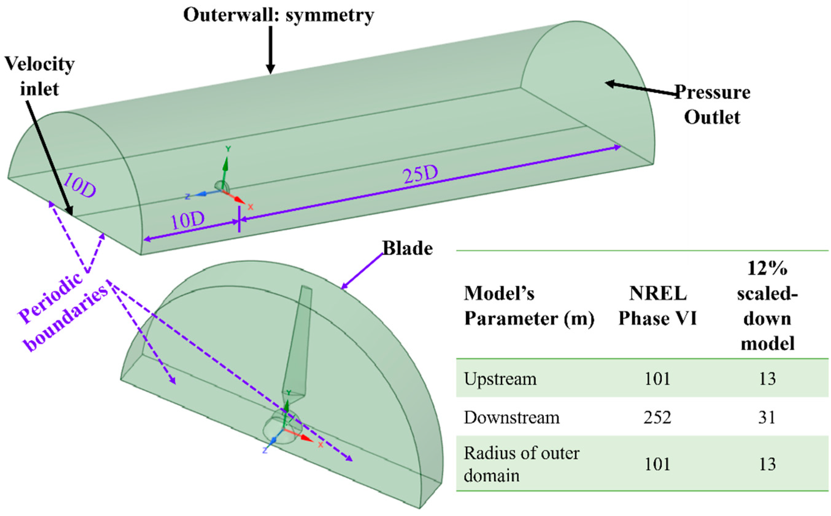
2.1. Computational Models

This study employed the NREL Phase VI horizontal-axis turbine geometry for numerical modeling. The reference geometry was stall-regulated, and the rotor was 10 m in diameter. An S809 airfoil was used for blade spans ranging in chord length from 0.25 m to 1 m. The transitional component joined the cylindrical portion of the blade with an airfoil. The details of the reference turbine geometry were presented by Hand et al. [8]. Only half of the turbine rotor was selected for the simulations to avoid an extensively heavy computational domain. The domains used in the simulations comprised two components: the inner rotating domain housing the turbine rotor and the outer stationary domain. Cylindrical domains were created owing to the rhythmic and periodic nature of the wind turbine rotor. The domain consisted of 10 times the diameter of the upstream side, 25 times the diameter of the downstream side, and a radius of 10 times the diameter of the turbine rotor. Similarly, the exact domain ratio was maintained for a 12% scaled-down turbine model, as shown in Figure 1. The upstream, downstream, and radius of the outer domain were selected as 101, 252, and 101 m for the full-scale model and 13, 31, and 13 m for the scaled-down model, respectively.

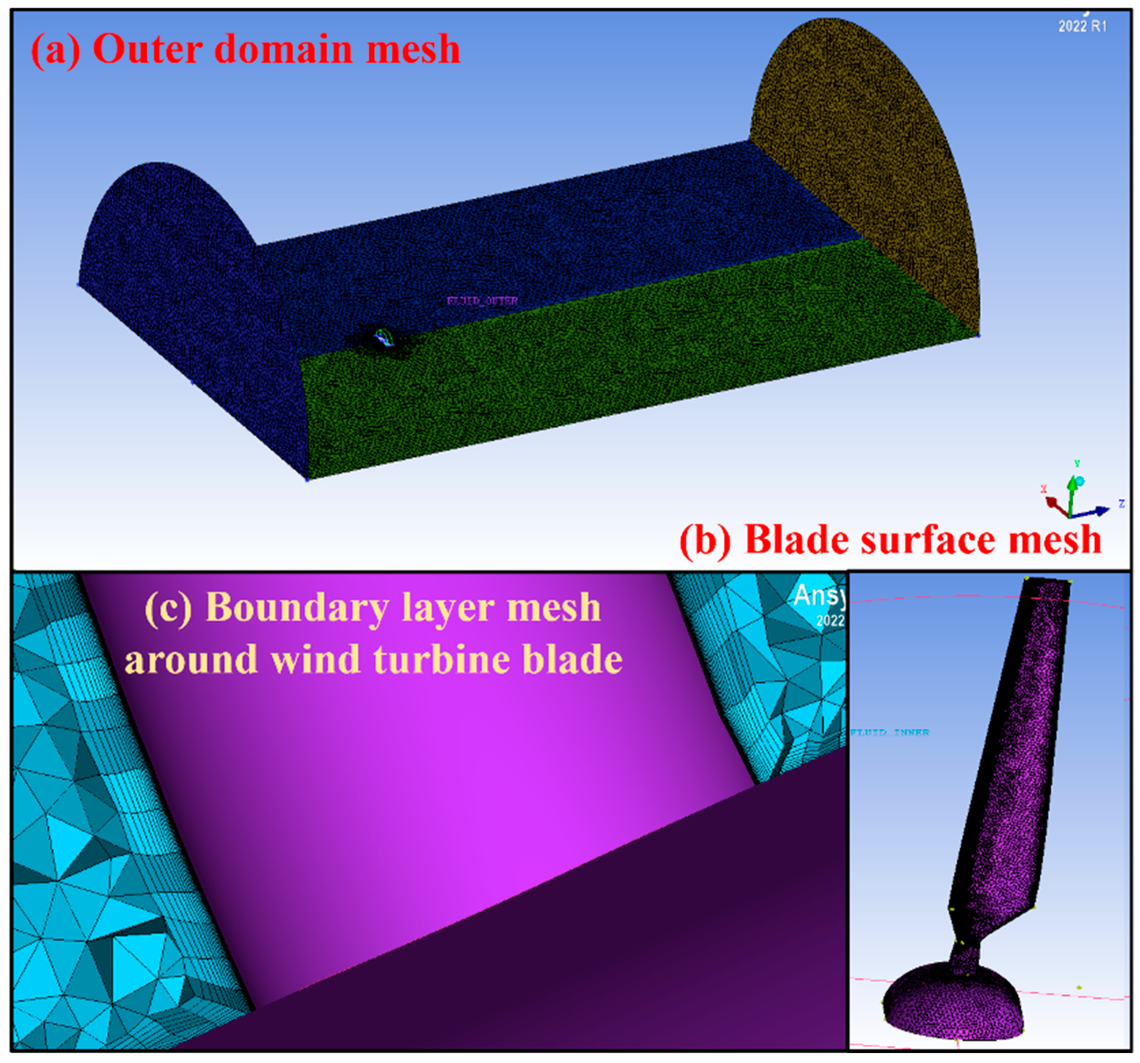
2.2. Meshing for CFD Simulation

This study explores the aerodynamic performance of wind turbine models; therefore, a refined mesh is required on blade surfaces. Specifically, a mesh found on both the leading and trailing edges was carefully considered owing to more curvatures in the geometry. A well-crafted unstructured mesh was generated using ICEM computational fluid dynamics based on local and global size parameters. To obtain Y+ < 1, an inflation layer containing 45 prisms with a growth rate of 1.25 and a prism ratio of 1.5 is redistributed at an initial height of 0.000015 mm for the geometry of the reference turbine blade. Similarly, 51 prism layers were generated at an initial height of 0.0000015 mm to analyze the flow dynamics near the blade surface for a scaled-down model. Many attempts have been made to obtain a Y+ value of less than one based on the initial heights. The Y+ value is determined as follows:
Y + = y p u t v
where y p   is the distance of the first element from the blade surface, ut is the friction velocity, and v is the kinematic viscosity [29].

2.3. Governing Equations and Theories of Turbulence

The calculations for the computational simulations were based on RANS and the continuity equation for compressible fluid flow. Shear stress transport (SST) and transitional shear stress transport turbulence models were applied to deal with the problem and compare the results. The following equations for mass and conservation were used [20,39]:
ρ t + x i ρ u i = 0
ρ u i t + ρ u i u j x i = p x i x i μ u i x j + u j x i 2 3 δ i j u i x i + x j ρ u i / u j / ¯ + ρ f i + F i
where f i denotes the body force; F i is a source term; µ is the fluid dynamic viscosity; and the Kronecker delta function is symbolized as δ i j , and it takes a value equal to one when i and j are equal and zero otherwise. The other term ρ u i / u j / ¯ represents the Reynolds stress tensor, where u i / and u j / represent fluctuating velocities. By applying the Boussinesq theory, the Reynolds stress can be formulated as follows:
ρ u i / u j / ¯ = μ t u i x j + u j x i 2 3 δ i j u k x k 2 3 ρ k δ i j
Here, k is the turbulent kinetic energy, and the eddy viscosity is expressed as μ t . The Reynolds stress is correlated to the turbulence, and the term ρ u i / u j / ¯ is determined using the turbulence model. The transition thickness and intermittency variables used in the equation are as follows [31,38]:
ρ γ t + ρ U j γ x j = P γ 1 E γ 1 + P γ 2 E γ 2 + x j μ + μ i σ x j x j
ρ R e θ t ~ t + ρ U j R e θ t ~ x i = P θ t + x i σ θ t μ + μ t σ γ R e θ t ~ x i
where the time-averaged velocity is represented by U j , µ is the dynamic viscosity, a i r   d e n s i t y   i s   d e n o t e d   b y   ρ , and the transition sources are denoted by Pγ and Eγ. The momentum thickness Reynolds number corresponds to R e θ t ~ , which is used to determine the transition point. γ is the intermittency variable in the equation used to locally initiate the transition.

2.4. Computational Parameters and Boundary Conditions

ANSYS Fluent 2022 R1 was used to perform the 3D unsteady state numerical simulations. The RANS equations were solved using the SST K-Omega and transitional SST models. The SIMPLE convergence algorithm facilitates the coupling of pressure and velocity. A second-order discretization scheme was applied to the convection and viscous terms in the governing equations. For three-dimensional unsteady numerical simulations, convergence was achieved with no appreciable change in the residuals while augmenting the iteration counts. Achieving residual normalization stability required a value of at least 1 × 10⁻⁷ for x, y, and z momentum; 1 × 10⁻⁶ for dissipation of turbulence and kinetic energy; and 1 × 10⁻⁵ for continuity. The velocity inlet was defined as an inlet for the simulation domain, and the outlet was defined as a pressure outlet, no-slip rotating condition for the blade surface, symmetry for the far-field, and 180-degree periodic boundary condition for periodicity, as shown in Figure 1.
NREL Phase VI operates as a stall-regulated turbine with a radius of 5.029 m, as measured at the NASA Ames wind tunnel. For the aerodynamic performance study, various data were gathered during the experimentation of the NREL Phase VI reference turbine [8]. This study adopted the reference turbine test sequence H measurements [7]. Wind velocities in the range of 5–25 m/s were used for the numerical simulations. In this range, the flow behaves differently: at low speed, the flow is fully attached; at medium speed, the flow remains attached to the inner part of the blade, and at high velocities, the flow is completely separated from the wind turbine blade’s surface.

2.5. Mesh Sensitivity Analysis

Computational mesh sensitivity and refinement analyses were performed based on three grid types: coarse, medium, and fine. A representative wind flow of 10 m/s with SST K-Omega and a transitional SST model based on the same scheme and topology was used. The total number of element reference model geometries was 19.3, 20.9, and 21.6 million for the three types of grids, respectively. Similarly, the total number of elements for the scaled-down model (12%) was 36.5, 38.6, and 42.5 million, respectively. The results of mesh size and grid sensitivity analyses are presented in Table 1 and shown in Figure 2.
The CFD solution must lie within the asymptotic convergence margin to evaluate the uncertainty. The mesh convergence ratio was defined to determine the asymptotic limit of convergence [40].
R c = k 12 k 23
Here, k 12 = m 1 m 2   a n d   k 23 = m 2 m 3 .
The torque values at the three grids were analyzed, and an Rc < 1. Similarly, the percentage variance between the fine and medium-mesh torque values was less than 2%. Therefore, a medium-mesh model was used to perform the simulations in this study.

3. Results and Discussion

In this section, we analyze and validate the torque, thrust force, and pressure coefficients for NREL Phase VI and the 12% scaled-down model. The simulation results were evaluated using experimental data for validation.

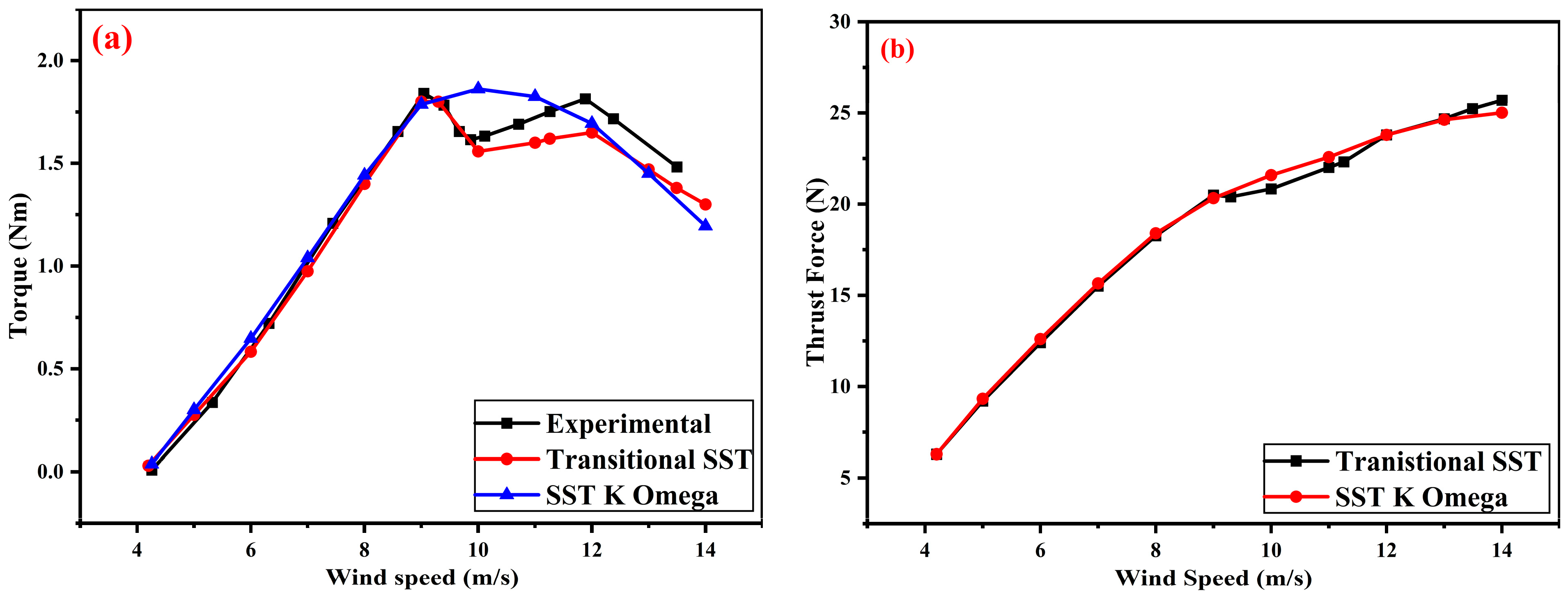
3.1. Torque and Thrust Force

The results obtained from the numerical simulations were cross-verified with the experimental measurements of sequence H obtained from a wind tunnel test performed at the NASA Amed wind tunnel for NREL Phase VI. The experimental values are represented by the actual values with bars of uncertainty [40,41]. Similarly, to verify the CFD models for a 12% scaled-down geometry, the torque values were compared with the available experimental data obtained at the Korea Aerospace Research Institute (KARI). The details of the operational parameters were consistent with the experimental work conducted by Cho et al. [41] to validate the numerical simulations. The torque can be defined as follows:
T = 1 2 ρ A s U R C m
where ρ is the density (1.225 kg/m3), A s is the rotor blade swept area, U∞ is the inlet velocity, R is the blade radius, and Cm is the moment coefficient estimated using CFD code.
As depicted in Figure 3a,b, the simulated findings obtained from the transitional shear stress transport and SST K-Omega turbulence models were validated with experimental data, and there was no considerable difference between wind velocities of 5 m/s and 10 m/s. At 10 m/s, both models overpredicted the torque values compared with the experimental results. The turbulence models provided an exceptional analogy with experimental data in the attached flow region but overestimated at the peak and underestimated the stall condition [42]. At 10 m/s, the maximum torque was observed at lower wind speeds before stalling at higher wind speeds. Above 10 m/s, the transitional SST model yielded more accurate results under stall conditions, up to a wind speed of 25 m/s. However, the simulated results of the transitional SST model fell below the experimental values but remained within the standard deviation measures. For wind speeds between 10 and 16 m/s, the SST K-Omega simulation results were in good agreement with the experimental values. However, after a wind flow velocity of 16 m/s, the full separation of the flow was evident, complex flow separation in the full stall region was not entirely captured in SST K-Omega, and poor performance was observed. The shear stress transport K-Omega model shows inadequacy at higher wind velocities for predicting the separation regions in uncertain flow separation. In general, the shear stress transport K-Omega model cannot correctly estimate the separation point [37]. Both the transitional SST and SST K-Omega models provided satisfactory predictions of the thrust force reasonably accurately based on the experimental data of the reference wind turbine (NREL Phase VI).
Similarly, the results obtained from the numerical simulation for torque and thrust force for the 12% scaled-down model turbine were validated with experimentally measured values for wind speed of 4 ms–14 m/s. As illustrated in Figure 4a, at wind flow velocities between 4 and 9 m/s, the simulated results of both the transitional SST and SST K-Omega models were in close agreement with the experimental values, even reaching a flow velocity of 10 m/s for the transitional SST model. At wind flow velocities of 10 and 11 m/s, the shear stress transport K-Omega turbulence model overpredicted the torque value. Above 11 m/s, the experimental and simulation results showed a difference of 2–7%. The transitional SST and SST K-Omega turbulence models showed reliable conformity with the experimental trend. As illustrated in Figure 4b, the thrust force calculated from the transitional SST and SST K-Omega turbulence models showed a similar trend, with an increase in flow velocities ranging from 4 m/s to 14 m/s.

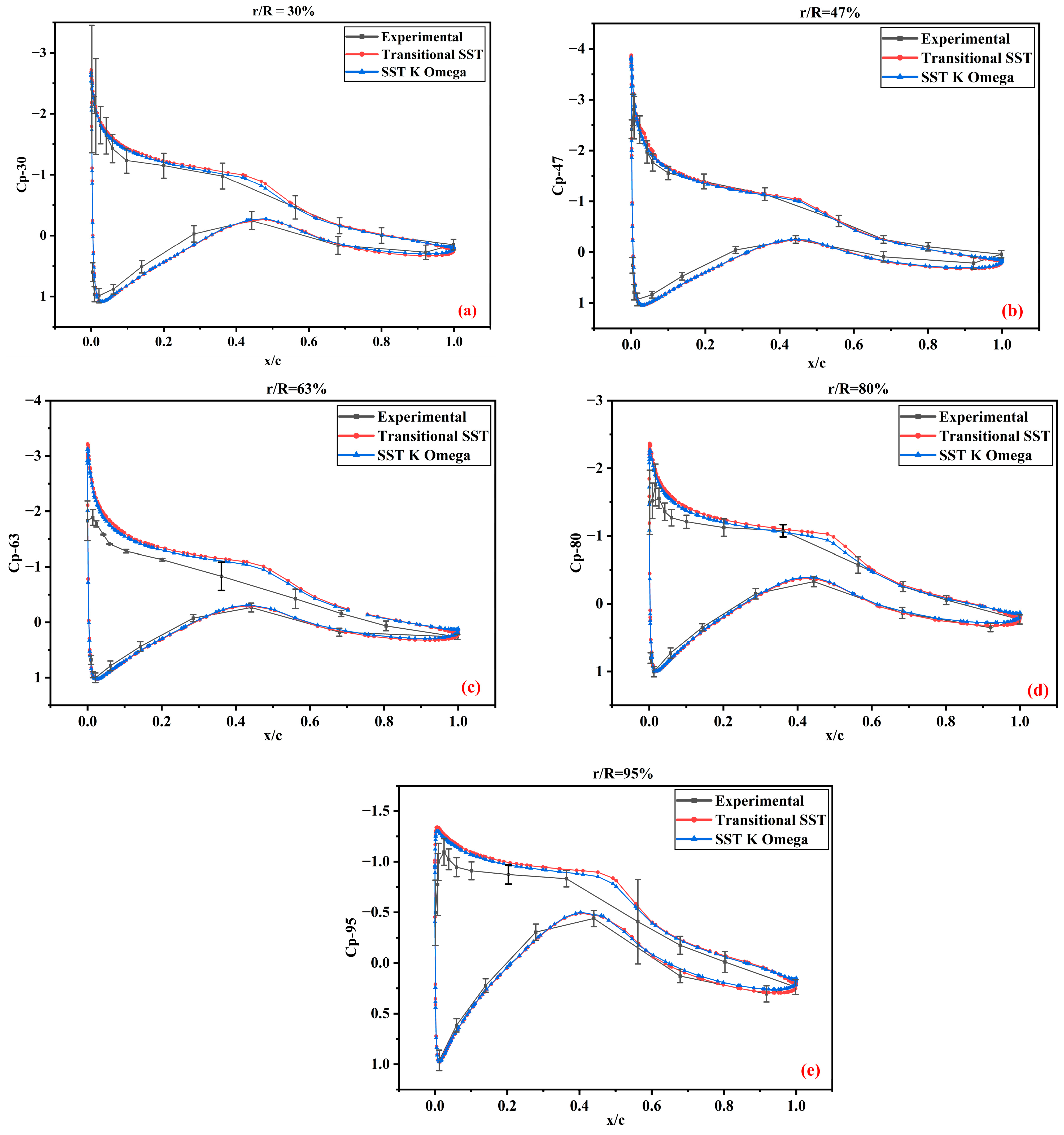
3.2. Pressure Coefficients

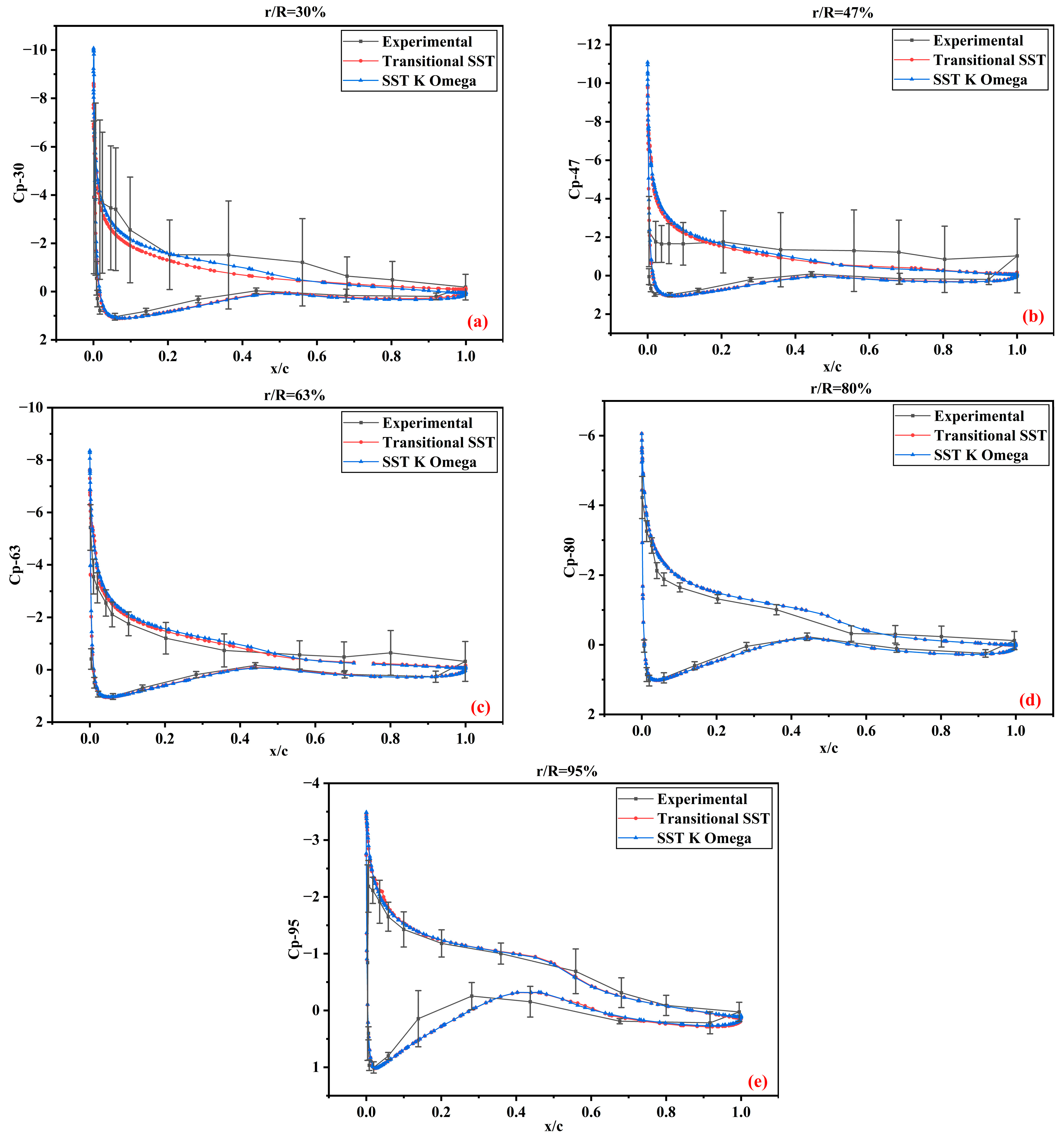
3.2.1. NREL Phase VI Validation

The validation of the simulation results in conjunction with the NREL Phase VI reference wind turbine was obtained from the experimental measurements of the test sequence at wind flow velocities of 7, 10, and 20 m/s, as illustrated in Figure 5, Figure 6, and Figure 7, respectively. Radial sections were considered for the NREL Phase VI reference turbine at blade spans of 30, 47, 63, 80, and 95%. The coefficient of pressure at any section of the turbine blade is defined as follows [20]:
C p = P P 1 2 ρ U 2 + r ω 2
where U∞ is the free stream velocity (m/s), r is the distance of the blade section from the root in meters, air density is represented as ρ in kilograms/cubic meters, ω is the angular velocity of the rotor in radians per second, the local pressure at any section is represented as P in pascal, and atmospheric pressure is expressed as P∞.
Figure 5 illustrates a comparative analysis of the pressure coefficient of the CFD simulation findings using the transitional SST and SST K-Omega turbulence models with the experimental data at a wind flow velocity of 7 m/s. The comparison showed a consistent trend in the CFD findings with the experimental data values in all sections. A marginal difference was observed between the CFD simulations and experimental results on the suction side at 63%, 80%, and 95% along the blade span, as shown in Figure 5c–e, respectively. The CFD simulation slightly overestimated the values of the blade suction side near the leading edge.
Figure 6 shows a comparison of the pressure coefficient of the CFD simulation results using the transitional SST and SST K-Omega turbulence models with the experimental results at a wind flow velocity of 10 m/s. When the flow velocity was 10 m/s, the results of the CFD simulation were consistent with the experimental measurements, with a slight difference between the simulated results of the transient shear stress transport model and the SST K-Omega model at 30% (Figure 6a) and 47% (Figure 6b) of the blade span, but they were within the standard deviation of the experimental data. At 80% (Figure 6d) of the blade section, there was a slight overestimation of the pressure in the CFD simulation along the suction side. At a blade span of 47%, the CFD results were underestimated when moving toward the trailing edge compared to the experimental data.
Figure 7 shows a comparison of the pressure coefficient of the CFD simulation results derived using the transitional SST and SST K-Omega turbulence models with the experimental results obtained at a wind speed of 20 m/s. When the wind speed was 20 m/s, the simulation results strongly agreed with the experimental results at the front side of the blade while increasing the pressure from extending to the trailing edge. Specifically, on the suction side, there was a distinction between the results obtained from the simulations and experiments. At 30% of the blade span (Figure 7a), the turbulence models underestimated the pressure coefficient values by up to 80% of the chord. At 47% (Figure 7b) of the blade span, the turbulence models underestimated the pressure coefficient value while moving toward the trailing edge. Similarly, different patterns were observed for the blade spans of 63% (Figure 7c), 80% (Figure 7d), and 95% (Figure 7e). However, all the simulation results were within the standard deviation range of the experimental data over the blade span.
Overall, both the transitional SST and SST K-Omega models provided good validation of the front surface of the blade using experimental data. Similarly, both turbulence models provided satisfactory results on the suction side while extending from the leading edge, except for some differences at a high inlet speed of 20 m/s. The trend behavior of the pressure variation at higher wind flow velocities, particularly at the suction side, is more prominent in the transitional SST turbulence model for the detection and localization of turbulent flow separation, as found at 63% and 95% spans of the blade.

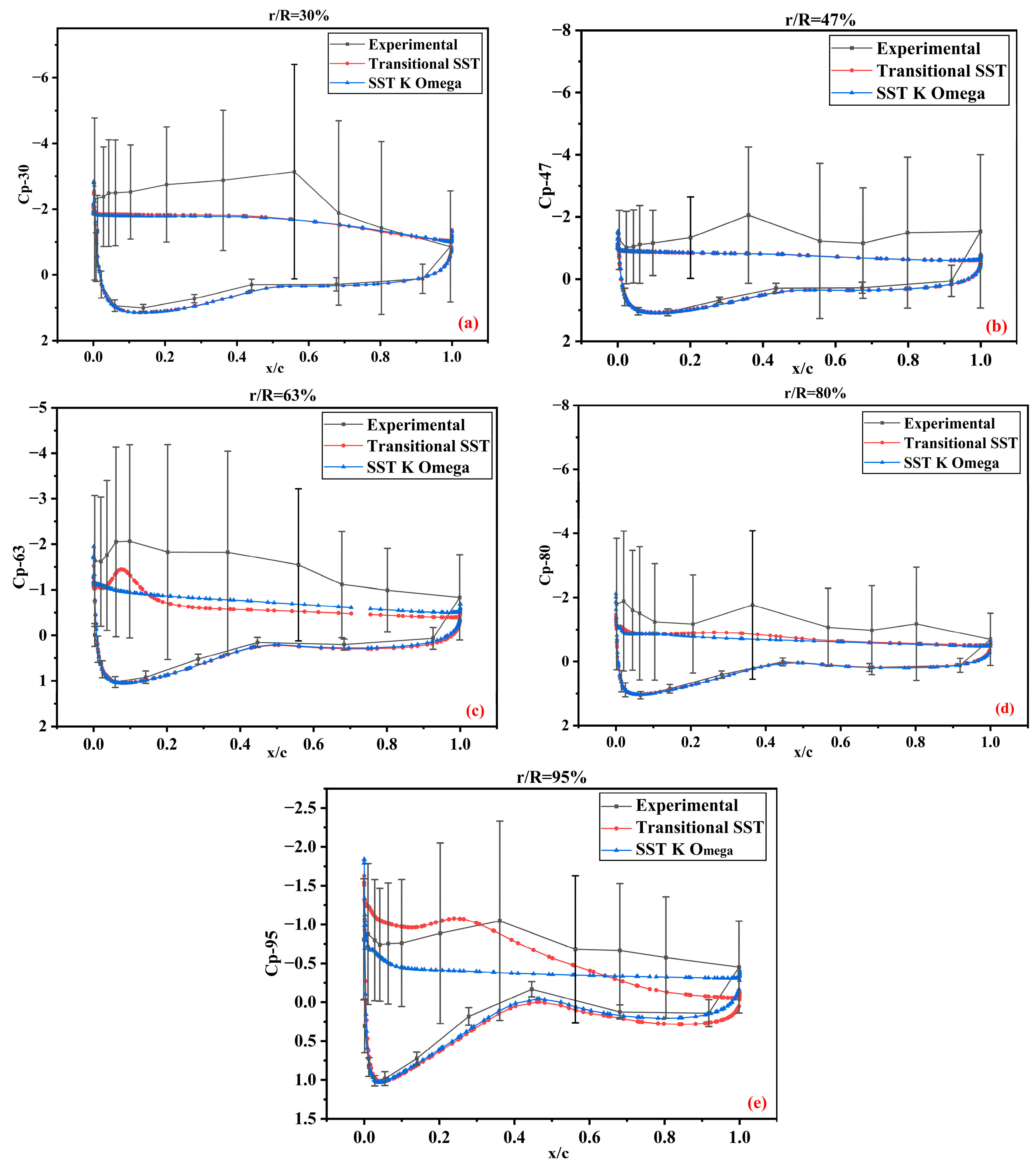
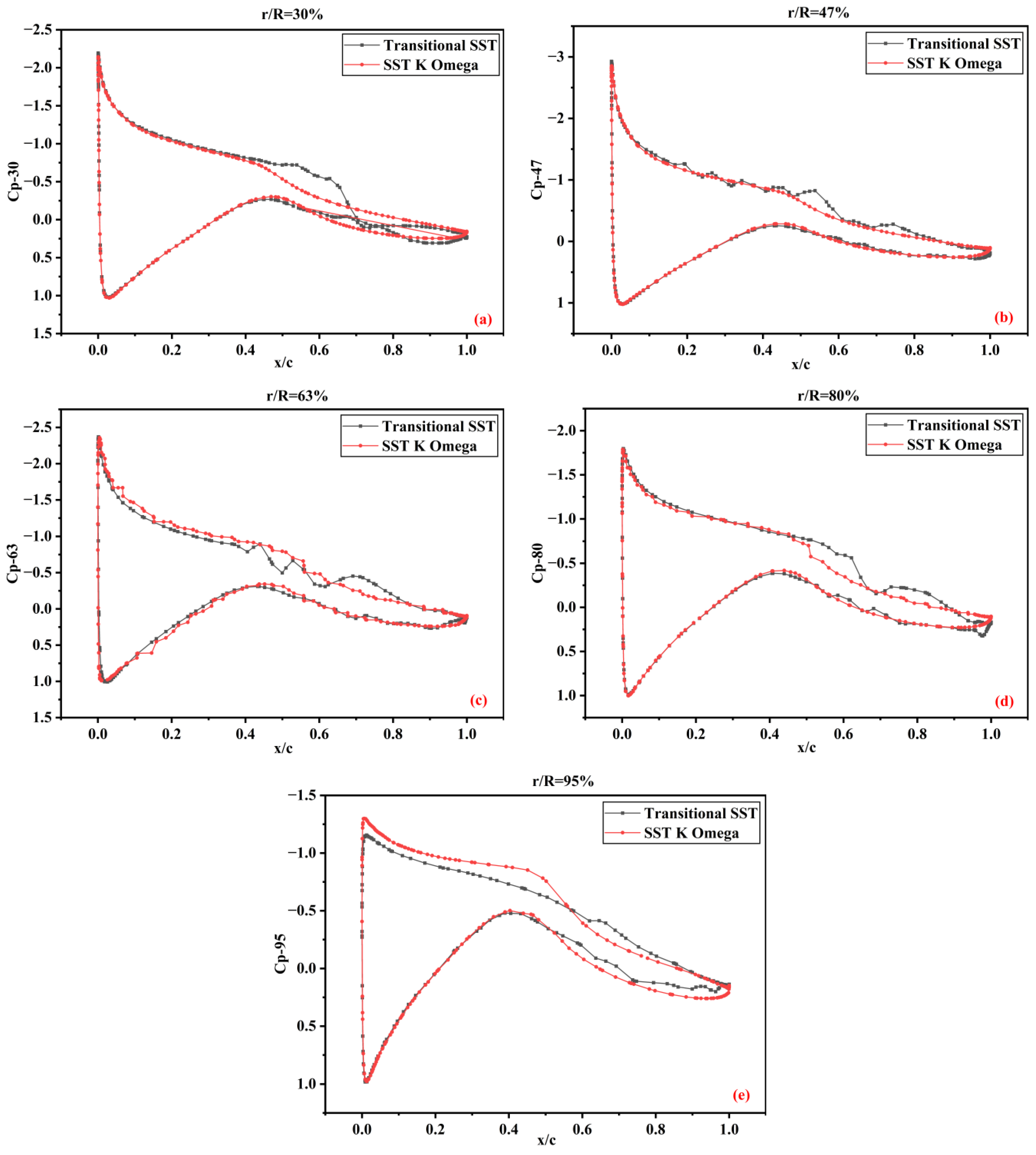
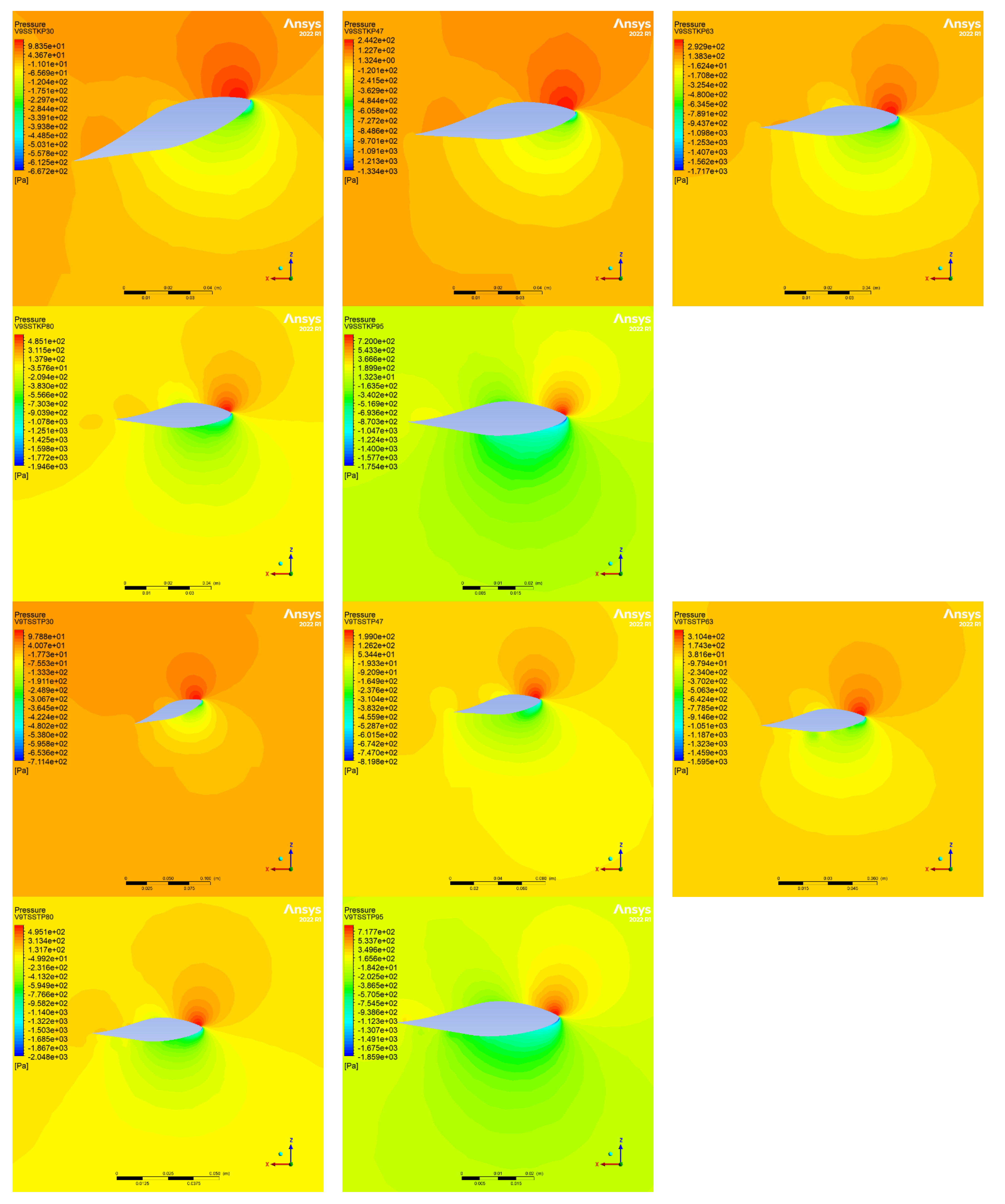
3.2.2. The 12% Scaled-Down Model

To the best of our knowledge, the aerodynamic performance analysis of the 12% scaled-down model is yet to be included in future research. The experimental data validated the torque values predicted by the transitional SST and SST K-Omega models. After validating the torque values with the reference experimental data, the coefficients of pressure at various spans of the model wind turbine were determined. The transitional SST and SST K-Omega models were applied to capture the flow variations that reflect the approximation of a full-scale turbine model based on aerodynamic scaling. Matching the tip speed ratio and Mach number in the scaled-down model ensures the replication of the wind and rotational speeds of the real turbine rotor. This section presents a detailed analysis of the pressure distribution accompanying the pressure coefficients of the 12% scaled-down model at wind flow velocities of 7, 9, and 12 m/s. Radial sections were considered for a 12% scaled-down wind turbine model with blade spans of 30, 47, 63, 80, and 95%. Figure 8, Figure 10, and Figure 12 show the results for the pressure coefficients. Figure 9, Figure 11, and Figure 13 show the variation in the pressure contours obtained from the transitional shear stress transport and shear stress transport K-Omega turbulence models, respectively.

At Wind Speed = 7 m/s

Figure 8 shows a comparison of the pressure coefficients predicted by the turbulence models for the selected wind velocity of 7 m/s. The simulation results at a wind speed of 7 m/s showed no marked deviation from the transitional shear stress transport model and the SST K-Omega model at the blade cross-section. Approximately 50% to 85% of the chord length and up to 80% (Figure 8d) of the blade span, there is a deviation in the results of the transitional shear stress transport model from the SST K-Omega model while moving toward the trailing edge, specifically at the suction side. At 95% (Figure 8e) of the blade span, the pressure coefficient values predicted by SST K-Omega were higher than those predicted by the transitional SST model in the suction region extending from the leading edge. After the midpoint of the chord on the front side of the blade, the transitional SST model yielded slightly higher values. The transitional SST model predicted the maximum pressure value on the blade span, except at a radial distance of 95% (Figure 8e). The pressure value was −968.2 pascal for the shear stress transport K-Omega model and −954.9 pascal for the transitional SST model located on the blade’s suction side. The pressure contours obtained from both turbulence models are shown in Figure 9.

At Wind Speed = 9 m/s

Figure 10 shows a comparison of the pressure coefficients predicted by both turbulence models at a selected wind flow velocity of 9 m/s. The numerical simulation results of the transitional SST model and SST K-Omega exhibit similar trends along the blade span. At a radial distance of 63% (Figure 10c), the transitional SST model captured the flow pattern better than SST K-Omega on the suction side of the blade covering from the leading edge to the trailing edge. Similarly, at a blade position of r/R = 95% (Figure 10e), local pressure was predicted well in the vicinity of the trailing edge in the transitional SST model in the suction region of the blade. The contours of the pressure distribution at 9 m/s of wind speed at different points along the blade are presented in Figure 11. The values of pressure obtained from the transitional SST model were higher at all span locations except at r/R = 47% (Figure 10b) radial distance. The maximum pressure value predicted by SST K-Omega was greater on both sides of the blade at a radial distance of 47%. (Figure 10b).

At Wind Speed = 12 m/s

The highest wind speed selected for the 12% scaled-down model was 12 m/s for the pressure analysis. Figure 12 shows a comparison of the pressure coefficients predicted by both turbulence models at a specified wind speed of 12 m/s. Figure 13 shows the contours of the pressure distribution on the front and suction sides of the blade for the SST K-Omega and transitional SST turbulence models, respectively. When the wind speed reached 12 m/s, the predictions of the pressure coefficient by both turbulence models were equal, except for some deviations along the suction region of the blade given by the transitional SST turbulence model. At r/R = 30%, the transitional SST model captured the flow separation more precisely than the SST K-Omega model. Similarly, at r/R = 80% (Figure 12c) and 95% (Figure 12e) of the blade span, the transitional SST model more precisely estimated the flow phenomena along the suction side of the blade. The SST K-Omega model provided the maximum pressure value in the suction regions at 95% of the blade radial span. The maximum pressure predicted by the transitional SST model was 715.2 pascal at r/R = 95% (Figure 12e). A comparison of the simulation results confirmed that the suction pressure increased, covering the distance from the bottom of the blade to its tip. The maximum suction was observed at r/R = 80% (Figure 12c) at wind flow speeds of 7 and 9 m/s. At high speeds, the maximum suction pressure was observed at r/R = 95% (Figure 12e), adjacent to the trailing edge of the blade. Similarly, the highest pressure and negative suction values were observed near the leading edge. The main concentration of suction pressure was adjacent to the leading edge, and the flow separated while moving toward the trailing edge of the blade. The pressure contours confirmed the reattachment close to the end of the blade tip. The maximum pressure observed was 927 pascals on the front side of the blade near the leading edge at a representative speed of 12 m/s.

4. Conclusions

This study validated the characteristics and aerodynamic performance of full-scale NREL Phase VI and 12% scaled-down models using the transitional SST and SST K-Omega turbulence models. The wind speeds varied from 5 to 25 m/s and 4 to 14 m/s, respectively. The representative wind speeds selected for this study were 7, 10, and 20 m/s for the full-scale model and 7, 9, and 12 m/s for the scaled-down model. Based on the results of the numerical simulations, the following conclusions were drawn:
  • For wind flow velocities in the range of 5–10 m/s, the numerical simulation results of the transitional SST and SST K-Omega models matched well with the experimental data of the torque and thrust force. At a wind velocity of 10 m/s, both turbulence models overestimated the torque and thrust force values. Likewise, the torque values estimated by both turbulence models for a 12% scaled-down model up to a wind speed of 9 m/s displayed excellent trends with the experimental results. At a wind speed of 9 m/s, flow separation from the blade surface was observed, and the numerical solutions of the transitional SST and SST K-Omega deviated from the experimental data. Overall, the transitional SST model matched reasonably well with the experimental trend and slightly underestimated the torque values after a wind speed of 10 m/s, with a difference of less than 6%.
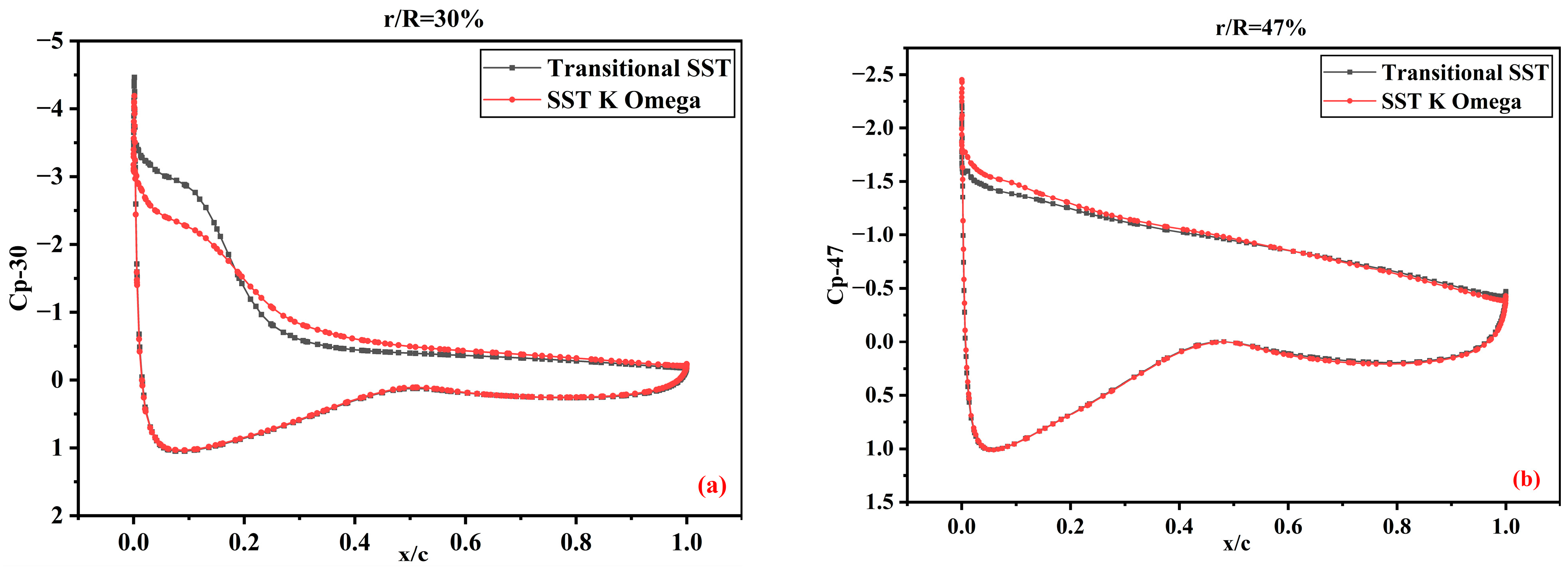
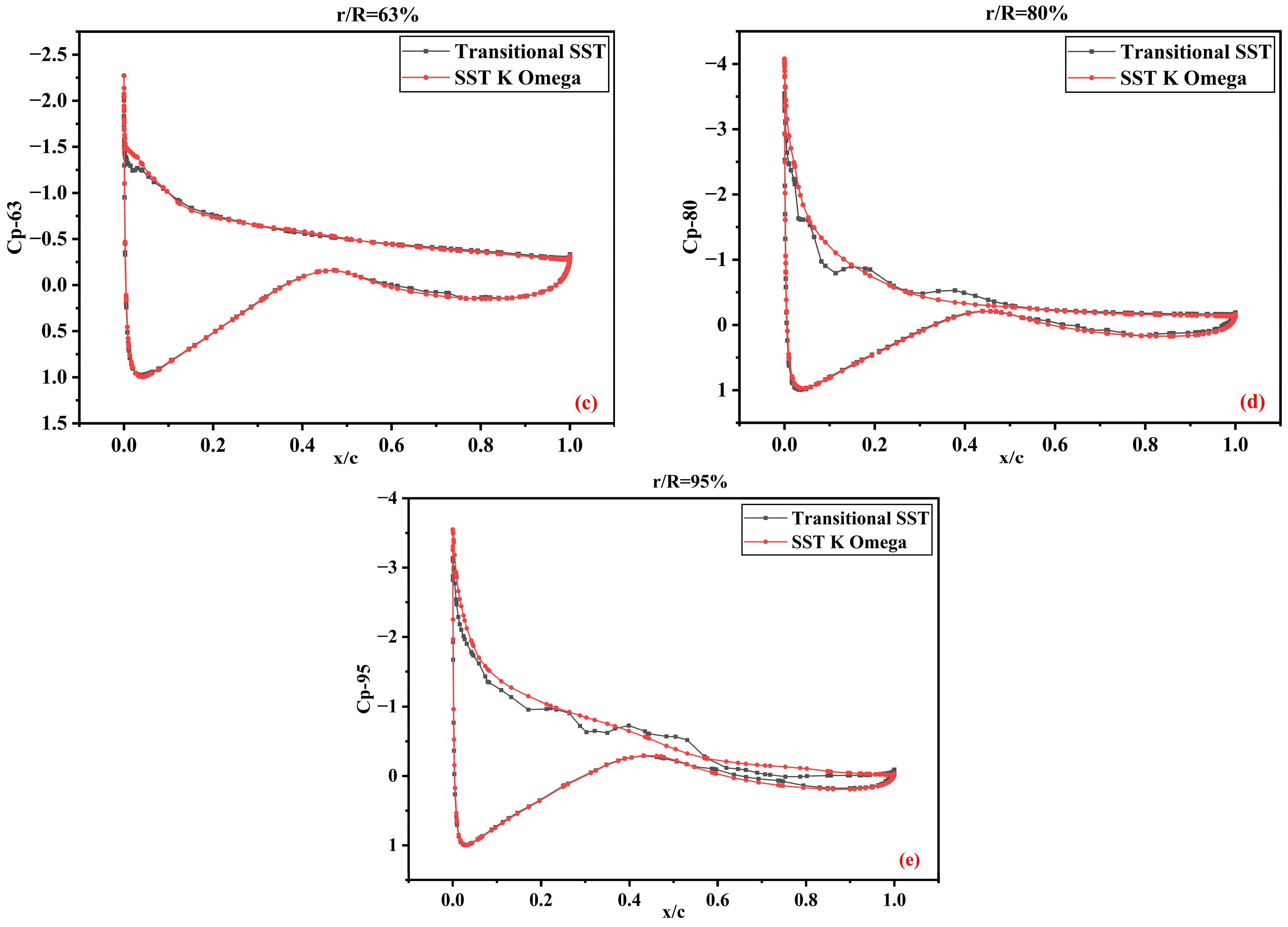
  • The pressure coefficients predicted by the transitional SST and SST K-Omega models show satisfactory agreement with the experimental data, except for some deviations at high speeds, but lie within the standard deviation of the experimental data.
  • The numerical results for the pressure coefficient curves obtained from the turbulence models were similar. The variation primarily occurred on the suction side, extending from the base to the blade tip. In the boundary layer region, the transitional SST model captured the flow phenomena better than the shear stress transport K-Omega model in the transition from the laminar to turbulent layers. Likewise, advancing from the leading edge to the trailing edge of the blade, the transitional SST model demonstrated an improved predicted flow separation. The simulation results of this study were limited to the specific flow regimes considered in the analysis.

5. Future Work

In the future, using the scaled-down model, the dynamic interaction of wind turbine blades, nacelles, and towers will be investigated to study their impact on performance and structural stability. Advanced measurement techniques and instrumentation will be developed to study fine-scale flow features and load dynamics.

Author Contributions

Conceptualization, Z.M. and Z.W.; methodology, Z.M.; software, Z.M.; validation, Z.M., Z.W. and X.Z.; formal analysis, Z.M. and X.Z.; investigation, Z.M. and G.S.; resources, Z.W.; data curation, Z.W.; writing—original draft preparation, Z.M.; writing—review and editing, Z.M. and G.S.; visualization, Z.M. and G.S.; supervision, Z.W.; project administration, Z.W. and X.Z.; funding acquisition, Z.W. All authors have read and agreed to the published version of the manuscript.

Funding

This study was financially supported by the National Natural Science Foundation of China (Grant Nos. 51779224 and 51579221) and the Basic Public Welfare Research Program of Zhejiang Province (Grant No. LHZ19E090002).

Data Availability Statement

The original contributions presented in the study are included in the article, further inquiries can be directed to the corresponding author.

Acknowledgments

The authors thank the National Renewable Energy Laboratory (NREL), United States Department of Energy, for providing experimental data to validate and verify the numerical results.

Conflicts of Interest

The authors declare no conflicts of interest.

References

  1. Panwar, N.L.; Kaushik, S.C.; Kothari, S. Role of renewable energy sources in environmental protection: A review. Renew. Sustain. Energy Rev. 2011, 15, 1513–1524. [Google Scholar] [CrossRef]
  2. Chehouri, A.; Younes, R.; Ilinca, A.; Perron, J. Review of performance optimization techniques applied to wind turbines. Appl. Energy 2015, 142, 361–388. [Google Scholar] [CrossRef]
  3. Veers, P.; Bottasso, C.L.; Manuel, L.; Naughton, J.; Pao, L.; Paquette, J.; Robertson, A.; Robinson, M.; Ananthan, S.; Barlas, T.; et al. Grand challenges in the design, manufacture, and operation of future wind turbine systems. Wind Energy Sci. 2023, 8, 1071–1131. [Google Scholar] [CrossRef]
  4. Zhong, J.; Li, J. Aerodynamic performance prediction of NREL phase VI blade adopting biplane airfoil. Energy 2020, 206, 118182. [Google Scholar] [CrossRef]
  5. Ye, M.; Chen, H.-C.; Koop, A. Verification and validation of CFD simulations of the NTNU BT1 wind turbine. J. Wind. Eng. Ind. Aerodyn. 2023, 234, 105336. [Google Scholar] [CrossRef]
  6. Geng, X.; Liu, P.; Hu, T.; Qu, Q.; Dai, J.; Lyu, C.; Ge, Y.; Akkermans, R.A. Multi-fidelity optimization of a quiet propeller based on deep deterministic policy gradient and transfer learning. Aerosp. Sci. Technol. 2023, 137, 108288. [Google Scholar] [CrossRef]
  7. Schreck, S.J. IEA Wind Annex XX: HAWT Aerodynamics and Models from Wind Tunnel Measurements; Final Report; National Renewable Energy Laboratory (NREL): Golden, CO, USA, 2008. [Google Scholar]
  8. Hand, M.M.; Simms, D.A.; Fingersh, L.J.; Jager, D.W.; Cotrell, J.R.; Schreck, S.; Larwood, S.M. Unsteady Aerodynamics Experiment Phase VI: Wind Tunnel Test Configurations and Available Data Campaigns; National Renewable Energy Laboratory (NREL): Golden, CO, USA, 2001. [Google Scholar]
  9. Giguère, P.; Selig, M.S. Design of a Tapered and Twisted Blade for the NREL Combined Experiment Rotor; National Renewable Energy Laboratory (NREL): Golden, CO, USA, 1999. [Google Scholar]
  10. Lyu, C.; Liu, P.; Hu, T.; Geng, X.; Qu, Q.; Sun, T.; Akkermans, R.A.D. Hybrid method for wall local refinement in lattice Boltzmann method simulation. Phys. Fluids 2023, 35, 017103. [Google Scholar] [CrossRef]
  11. Lyu, C.; Liu, P.; Hu, T.; Geng, X.; Sun, T.; Akkermans, R.A. A sliding mesh approach to the Lattice Boltzmann Method based on non-equilibrium extrapolation and its application in rotor flow simulation. Aerosp. Sci. Technol. 2022, 128, 107755. [Google Scholar] [CrossRef]
  12. Menter, F.R. Two-equation eddy-viscosity turbulence models for engineering applications. AIAA J. 1994, 32, 1598–1605. [Google Scholar] [CrossRef]
  13. Wilcox, D.C.; Suga, K. Turbulence Modelling for CFD; DCW Industries Inc.: La Cañada, CA, USA, 1993; p. 460. [Google Scholar]
  14. Lee, K.; Huque, Z.; Kommalapati, R.; Han, S.-E. Fluid-structure interaction analysis of NREL phase VI wind turbine: Aerodynamic force evaluation and structural analysis using FSI analysis. Renew. Energy 2017, 113, 512–531. [Google Scholar] [CrossRef]
  15. Song, Y.; Perot, J.B. CFD Simulation of the NREL Phase VI Rotor. Wind. Eng. 2015, 39, 299–309. [Google Scholar] [CrossRef]
  16. Wang, P.; Liu, Q.; Li, C.; Miao, W.; Yue, M.; Xu, Z. Investigation of the aerodynamic characteristics of horizontal axis wind turbine using an active flow control method via boundary layer suction. Renew. Energy 2022, 198, 1032–1048. [Google Scholar] [CrossRef]
  17. Dias, M.M.G.; Ramirez Camacho, R.G. Optimization of NREL phase VI wind turbine by introducing blade sweep, using CFD integrated with genetic algorithms. J. Braz. Soc. Mech. Sci. Eng. 2022, 44, 52. [Google Scholar] [CrossRef]
  18. Lee, M.-H.; Shiah, Y.C.; Bai, C.-J. Experiments and numerical simulations of the rotor-blade performance for a small-scale horizontal axis wind turbine. J. Wind. Eng. Ind. Aerodyn. 2016, 149, 17–29. [Google Scholar] [CrossRef]
  19. Sedighi, H.; Akbarzadeh, P.; Salavatipour, A. Aerodynamic performance enhancement of horizontal axis wind turbines by dimples on blades: Numerical investigation. Energy 2020, 195, 117056. [Google Scholar] [CrossRef]
  20. Ke, W.; Hashem, I.; Zhang, W.; Zhu, B. Influence of leading-edge tubercles on the aerodynamic performance of a horizontal-axis wind turbine: A numerical study. Energy 2022, 239, 122186. [Google Scholar] [CrossRef]
  21. Menegozzo, L.; Monte, A.D.; Benini, E.; Benato, A. Small wind turbines: A numerical study for aerodynamic performance assessment under gust conditions. Renew. Energy 2018, 121, 123–132. [Google Scholar] [CrossRef]
  22. International Electrotechnical Commission. Wind Turbines–Part 2: Design Requirements for Small Wind Turbines; Technical Report 61400-2; International Electrotechnical Commission: Geneva, Switzerland, 2013. [Google Scholar]
  23. Radünz, W.C.; Sakagami, Y.; Haas, R.; Petry, A.P.; Passos, J.C.; Miqueletti, M.; Dias, E. Influence of atmospheric stability on wind farm performance in complex terrain. Appl. Energy 2021, 282, 116149. [Google Scholar] [CrossRef]
  24. Seim, F.; Gravdahl, A.R.; Adaramola, M.S. Validation of kinematic wind turbine wake models in complex terrain using actual windfarm production data. Energy 2017, 123, 742–753. [Google Scholar] [CrossRef]
  25. Subramanian, B.; Chokani, N.; Abhari, R. Aerodynamics of wind turbine wakes in flat and complex terrains. Renew. Energy 2016, 85, 454–463. [Google Scholar] [CrossRef]
  26. Zhao, F.; Gao, Y.; Wang, T.; Yuan, J.; Gao, X. Experimental Study on Wake Evolution of a 1.5 MW Wind Turbine in a Complex Terrain Wind Farm Based on LiDAR Measurements. Sustainability 2020, 12, 2467. [Google Scholar] [CrossRef]
  27. Liu, Z.; Liu, P.; Guo, H.; Hu, T. Experimental investigations of turbulent decaying behaviors in the core-flow region of a propeller wake. Proc. Inst. Mech. Eng. Part G J. Aerosp. Eng. 2020, 234, 319–329. [Google Scholar] [CrossRef]
  28. Menter, F.R.; Langtry, R.B.; Likki, S.R.; Suzen, Y.B.; Huang, P.G.; Völker, S. A Correlation-Based Transition Model Using Local Variables—Part I: Model Formulation. J. Turbomach. 2004, 128, 413–422. [Google Scholar] [CrossRef]
  29. Lanzafame, R.; Mauro, S.; Messina, M. Wind turbine CFD modeling using a correlation-based transitional model. Renew. Energy 2013, 52, 31–39. [Google Scholar] [CrossRef]
  30. Sihag, S.; Kumar, M.; Tiwari, A.K. CFD Validation and Aerodynamic Behaviour of NREL Phase VI Wind Turbine. IOP Conf. Ser. Mater. Sci. Eng. 2022, 1248, 012063. [Google Scholar] [CrossRef]
  31. Ji, B.; Zhong, K.; Xiong, Q.; Qiu, P.; Zhang, X.; Wang, L. CFD simulations of aerodynamic characteristics for the three-blade NREL Phase VI wind turbine model. Energy 2022, 249, 123670. [Google Scholar] [CrossRef]
  32. Langtry, R.; Gola, J.; Menter, F. Predicting 2D Airfoil and 3D Wind Turbine Rotor Performance using a Transition Model for General CFD Codes. In Proceedings of the 44th AIAA Aerospace Sciences Meeting and Exhibit, Reno, NV, USA, 9–12 January 2006. [Google Scholar]
  33. Blocken, B.; van Druenen, T.; Toparlar, Y.; Andrianne, T. Aerodynamic analysis of different cyclist hill descent positions. J. Wind. Eng. Ind. Aerodyn. 2018, 181, 27–45. [Google Scholar] [CrossRef]
  34. Kato, M. The Modeling of Turbulent Flow Around Stationary and Vibrating Square Cylinders. In Proceedings of the 9th International Symposium on Turbulent Shear Flows, Kyoto, Japan, 16–18 August 1993. [Google Scholar]
  35. Shaik, M.; Subramanian, B. Computational investigation of NREL Phase-VI rotor: Validation of test sequence-S measurements. Wind Eng. 2023, 47, 973–994. [Google Scholar] [CrossRef]
  36. Amiri, M.M.; Shadman, M.; Estefen, S.F. URANS simulations of a horizontal axis wind turbine under stall condition using Reynolds stress turbulence models. Energy 2020, 213, 118766. [Google Scholar] [CrossRef]
  37. Moshfeghi, M.; Song, Y.J.; Xie, Y.H. Effects of near-wall grid spacing on SST-K-ω model using NREL Phase VI horizontal axis wind turbine. J. Wind. Eng. Ind. Aerodyn. 2012, 107–108, 94–105. [Google Scholar] [CrossRef]
  38. Younoussi, S.; Ettaouil, A. Numerical Study of a Small Horizontal-Axis Wind Turbine Aerodynamics Operating at Low Wind Speed. Fluids 2023, 8, 192. [Google Scholar] [CrossRef]
  39. Pope, S.B. Turbulent Flows; Cambridge University Press: Cambridge, UK, 2000. [Google Scholar]
  40. Stern, F.; Wilson, R.; Shao, J. Quantitative V&V of CFD simulations and certification of CFD codes. Int. J. Numer. Methods Fluids 2006, 50, 1335–1355. [Google Scholar]
  41. Cho, T.; Kim, C.; Lee, D. Acoustic measurement for 12% scaled model of NREL Phase VI wind turbine by using beamforming. Curr. Appl. Phys. 2010, 10 (Suppl. S2), S320–S325. [Google Scholar] [CrossRef]
  42. Hartwanger, D.; Horvat, A. 3D Modelling of a Wind Turbine Using CFD. In Proceedings of the NAFEMS UK Conference “Engineering Simulation: Effective Use and Best Practice”, Cheltenham, UK, 10–11 June 2008. [Google Scholar]
Figure 1. Details of the domain used for the CFD simulation.
Energies 17 05449 g001
Figure 2. Meshing for simulations.
Energies 17 05449 g002
Figure 3. Comparison of torque (a) and thrust force (b) using CFD and experimental data for NREL Phase VI.
Energies 17 05449 g003
Figure 4. Comparison of torque (a) and thrust force (b) using CFD and experimental data for the scaled-down model based on NREL Phase VI.
Energies 17 05449 g004
Figure 5. Comparison of the coefficient of pressure of NREL Phase VI obtained from CFD simulations and experimental data at a free-stream velocity of 7 m/s and at different blade sections (ae).
Energies 17 05449 g005
Figure 6. Comparison of the coefficient of pressure of NREL Phase VI obtained from CFD simulations and experimental data at a free-stream velocity of 10 m/s and at different blade sections (ae).
Energies 17 05449 g006
Figure 7. Comparison of the coefficient of pressure of NREL Phase VI obtained from CFD simulations and experimental data at a free-stream velocity of 20 m/s and at different blade sections (ae).
Energies 17 05449 g007
Figure 8. Comparison of pressure coefficients obtained from transitional SST and SST K-Omega turbulence models at a wind velocity of 7 m/s and at different blade sections (ae).
Energies 17 05449 g008
Figure 9. Pressure variation contours at different radial locations of the blade by SST K-Omega (graph with title SSTKP) and transitional SST (graph with title TSSTP) models at a wind velocity of =7 m/s.
Energies 17 05449 g009
Figure 10. Comparison of pressure coefficients obtained from transitional SST and SST K-Omega turbulence models at a wind speed of 9 m/s and at different blade sections (ae).
Energies 17 05449 g010
Figure 11. Pressure variation contours at different radial locations of the blade using SST K-Omega (graph with title SSTKP) and transitional SST (graph with title TSSTP) models at a wind speed of 9 m/s.
Energies 17 05449 g011
Figure 12. Comparison of pressure coefficients obtained from SST K-Omega and transitional SST models at a wind speed of 12 m/s and at different blade sections (ae).
Energies 17 05449 g012aEnergies 17 05449 g012b
Figure 13. Pressure variation contours at different radial locations of the blade using SST K-Omega (graph with title SSTKP) and transitional SST (graph with title TSSTP) models at a wind speed of 12 m/s.
Energies 17 05449 g013aEnergies 17 05449 g013b
Table 1. Grid sensitivity analysis.
Model NameMeshMesh Size (Million)Torque (Nm)RC
NREL Phase VI m 3 : Coarse19.31607.680.035
m 2 : Medium20.91686.50
m 1 : Fine21.61689.32
12% Scaled Down m 3 : Coarse36.50.7106640.030
m 2 : Medium38.60.834985
m 1 : Fine42.50.849573
Disclaimer/Publisher’s Note: The statements, opinions and data contained in all publications are solely those of the individual author(s) and contributor(s) and not of MDPI and/or the editor(s). MDPI and/or the editor(s) disclaim responsibility for any injury to people or property resulting from any ideas, methods, instructions or products referred to in the content.

