Enhancing Regional Wind Power Forecasting through Advanced Machine-Learning and Feature-Selection Techniques

Abstract

In this study, an in-depth analysis is presented on forecasting aggregated wind power production at the regional level, using advanced Machine-Learning (ML) techniques and feature-selection methods. The main problem consists of selecting the wind speed measuring points within a large region, as the wind plant locations are assumed to be unknown. For this purpose, the main cities (province capitals) are considered as possible features and four feature-selection methods are explored: Pearson correlation, Spearman correlation, mutual information, and Chi-squared test with Fisher score. The results demonstrate that proper feature selection significantly improves prediction performance, particularly when dealing with high-dimensional data and regional forecasting challenges. Additionally, the performance of five prominent machine-learning models is analyzed: Long Short-Term Memory (LSTM) networks, Artificial Neural Networks (ANNs), Support Vector Machines (SVMs), Convolutional Neural Networks (CNNs), and Extreme-Learning Machines (ELMs). Through rigorous testing, LSTM is identified as the most effective model for the case study in northern Italy. This study offers valuable insights into optimizing wind power forecasting models and underscores the importance of feature selection in achieving reliable and accurate predictions.

1. Introduction

The increasing dependence on renewable energy sources is essential to meet the rising global energy demand, which is expected to exceed 10 billion by 2050 [1]. Renewable energy sources, such as wind, solar, and hydro-power, offer sustainable alternatives to depleting fossil fuels, significantly reducing environmental pollution and mitigating the adverse effects of climate change [2]. Recent technological advancements have made renewable energy technologies more economically viable and improved integration into the energy market [1]. Accurately predicting wind power generation is crucial for maintaining the balance between supply and demand in electricity systems, yet the inherent variability of wind resources complicates this task [3,4]. Fuzzy models [5], as demonstrated in various applications, provide an effective means for managing uncertainty and nonlinearity in complex systems, making them particularly advantageous for ultra-short-term wind speed and power forecasting. A two-stage fuzzy nonlinear fusion model, using empirical mode decomposition and T-S fuzzy models combined with IT2-based aggregation, has demonstrated superior accuracy in ultra-short-term forecasting for wind farms in Colorado, USA [6]. A data-driven probabilistic Wind Power Ramps WPR forecasting (p-WPRF) method has been developed in [7], utilizing machine learning and a generalized Gaussian mixture model to predict wind power ramp events with high accuracy. A model employing meteorological data and fuzzy c-means clustering have demonstrated improved accuracy over traditional methods [8]. Additionally, in [9], a two-stage adaptive approach combining the Hilbert transform and neural networks has been proposed for forecasting nonstationary time series, showing effectiveness in managing highly variable power flows. Enhanced versions of SVM, like those combined with optimization algorithms such as the improved dragonfly algorithm, have demonstrated superior prediction performance compared to traditional models like Back Propagation Neural Networks (BPNNs) and Gaussian process regression [10]. ELM, known for its fast training times and high accuracy, outperforms classical ANNs in both short-term and multi-step-ahead forecasting scenarios, especially in complex terrains [11]. LSTM networks, a type of Recurrent Neural Network (RNN), excel in capturing temporal dependencies in wind speed data, providing robust short-term predictions [12]. CNNs, often used in hybrid models with other deep-learning techniques like Gated Recurrent Units (GRUs), automatically extract complex spatial features from wind power data, enhancing prediction accuracy [13]. Other notable models include the hybrid deep-learning approaches such as Variable Mode Decomposition (VMD)-CNN-GRU, which combine various techniques to reduce volatility and improve both short-term and long-term forecasting accuracy [14].

When the aggregated wind power in a large region is to be predicted, a standard approach is to aggregate the single power forecasts of all wind plants within the region. This approach has many disadvantages. One significant issue is obtaining real-time power generation data from all wind power plants, as many offline plants lack the necessary infrastructure for continuous data collection [15]. Additionally, the spatial and temporal correlations between different wind farms must be accurately captured [13]. The high-dimensional feature sets often encountered in regional forecasting further complicate the process, necessitating feature-selection and reduction techniques to manage redundant information [16]. Moreover, the variability in meteorological conditions across large areas demands robust models capable of integrating numerical weather predictions with historical data to enhance forecast accuracy [17]. Advanced forecasting methods are essential for handling the uncertainty in wind power predictions, but they introduce additional challenges in model construction and data processing [18]. Obviously, in this context, feature selection is pivotal, and advanced feature-selection methods allow for better determination of the significance and stability of various features, significantly enhancing forecasting model performance [19,20]. These methods streamline input data, for example by clustering features into sets and mapping them onto graphs or using PCA to reduce dimensionality and eliminate non-informative features [19,21,22]. The importance of feature selection is further underscored in [23], where deep feature-selection frameworks ensure that only the most pertinent data influences the initial layer of ML models. A PV power prediction method, presented in [24], is based on the Pearson coefficient and addresses factors such as ambient temperature, relative humidity, and solar irradiance by using correlation tests to remove irrelevant features while using an LSTM network. Similarly, ref. [25] employs LSTM neural networks for ultra-short-term prediction, and the Spearman rank correlation is used to determine hyper-parameters, for high-precision wind power forecasting in a wind farm in western China.

Most of the papers cited address the problem of hourly predicting the production of a single wind farm, even in the case of regional forecasts, which are obtained as the sum of the predictions at every single plant. In this kind of task, the problem is well defined: the output to be predicted is the plant power, while the input is the predicted wind speed and direction in the geographical position of the plant (more than one wind measurement point may be considered for very large plants).

This research faces a different and more complex task: the hourly prediction of aggregated wind energy production in a very large region, such as northern Italy, while considering the positions of the wind plants and their production to be unknown. This is a completely different task because there is a single known aggregated power to be predicted as an output, but detailed information about each plant in the region cannot be obtained. The region is too large, and acquiring real-time power generation data from all wind power plants within it presents a significant challenge. Thus, while there is a well-defined output to be predicted, the input is not well-defined.

In this work, a new approach is proposed to select the “input points” (denoted as measurement points) by identifying the main cities (province capitals in Italy) of the region. Additionally, since the capital cities comprise a substantial number (47 in the northern region of Italy), an exhaustive comparison of several feature-selection techniques is performed to reduce the number of input features. Furthermore, many state-of-the-art machine-learning and deep-learning regression methods are compared.

The research begins by highlighting the specific challenges of accurately predicting wind power at the regional level, followed by an introduction to the case under study. A range of machine-learning methods is explored, including SVM, ANN, ELM, CNN, and LSTM networks. Preliminary predictions will be made using these methods to identify the most effective approach for this case. Then, various feature-selection techniques are assessed, such as mutual information, Spearman correlation, Pearson correlation, the Chi-squared test, and Fisher score. Based on established criteria, the most suitable feature-selection method will be selected and applied to improve wind power forecasts in the region. By demonstrating the impact of refined feature selection, this comprehensive approach aims to enhance the accuracy and reliability of load predictions for regional wind power plants.

2. Problem Description: Regional Wind Power Forecasting with Unknown Plant Position and Production Data

Wind speed is the most significant factor influencing turbine output, with power generation increasing proportionally to the cube of wind speed. However, factors like turbulence, wind direction, and air density introduce additional complexity. Turbulence can reduce power output and increase stress on turbine components, while deviations in wind direction and yaw misalignment affect the performance of turbines across wind farms [26,27]. Moreover, air density, influenced by temperature and pressure, plays an essential role in power generation but was excluded from this study due to discrepancies in measurement locations [28].

The primary challenge in regional forecasting is the limited availability of detailed data for each wind power plant. In this case, only wind speed and temperature data are available for specific points, which may not correspond closely to the locations of the wind plants. As a result, precise predictions for individual plants are not feasible within this framework.

Regional forecasting, while less accurate on a plant-specific level, offers practical advantages by addressing broader areas with more efficiency. Therefore, this study aims to enhance the accuracy of regional wind power forecasts by employing advanced feature-selection techniques, providing a more scalable approach to predicting power production across multiple wind farms.

The main contribution of this study is a proposed approach to select the measuring points (locations) within a large geographical area in order to predict the aggregated power produced from the wind resource in that area (considering unknown locations of the wind plants). Wind speed forecasts at these locations are acquired from a provider such as Aeronautica Militare. The machine-learning methods are then used to relate the gathered wind speeds from several locations to the single aggregated power of the region. The time horizon is fixed to 24 h, as it is the value useful for the day before the market, which is where this aggregated forecast is mostly supposed to be used, other than defining power flows and unit commitment.

3. Case Study Description

The case study in this work focuses on a zone in northern Italy that includes the provinces of Emilia Romagna, Veneto, Friuli Venezia Giulia, Trentino Alto Adige, Lombardy, Piedmont, Liguria, and Aosta Valley. Within this region, access is available to the total production power of all wind power plants; however, specific details about the production capacities of individual power plants are unavailable. Additionally, meteorological data, including wind speed and temperature, are available for 47 locations, corresponding to the most important cities in this zone [29,30]. The available data spans from 20 January 2022 to 20 March 2023, with a granularity of one hour.

Hourly wind speed data are available for all 47 most important cities, with each dataset divided into two components: ugrd_10m, wind speed along the x-axis or the east–west direction (m/s), and vgrd_10m, wind speed along the y-axis or the north–south direction (m/s).

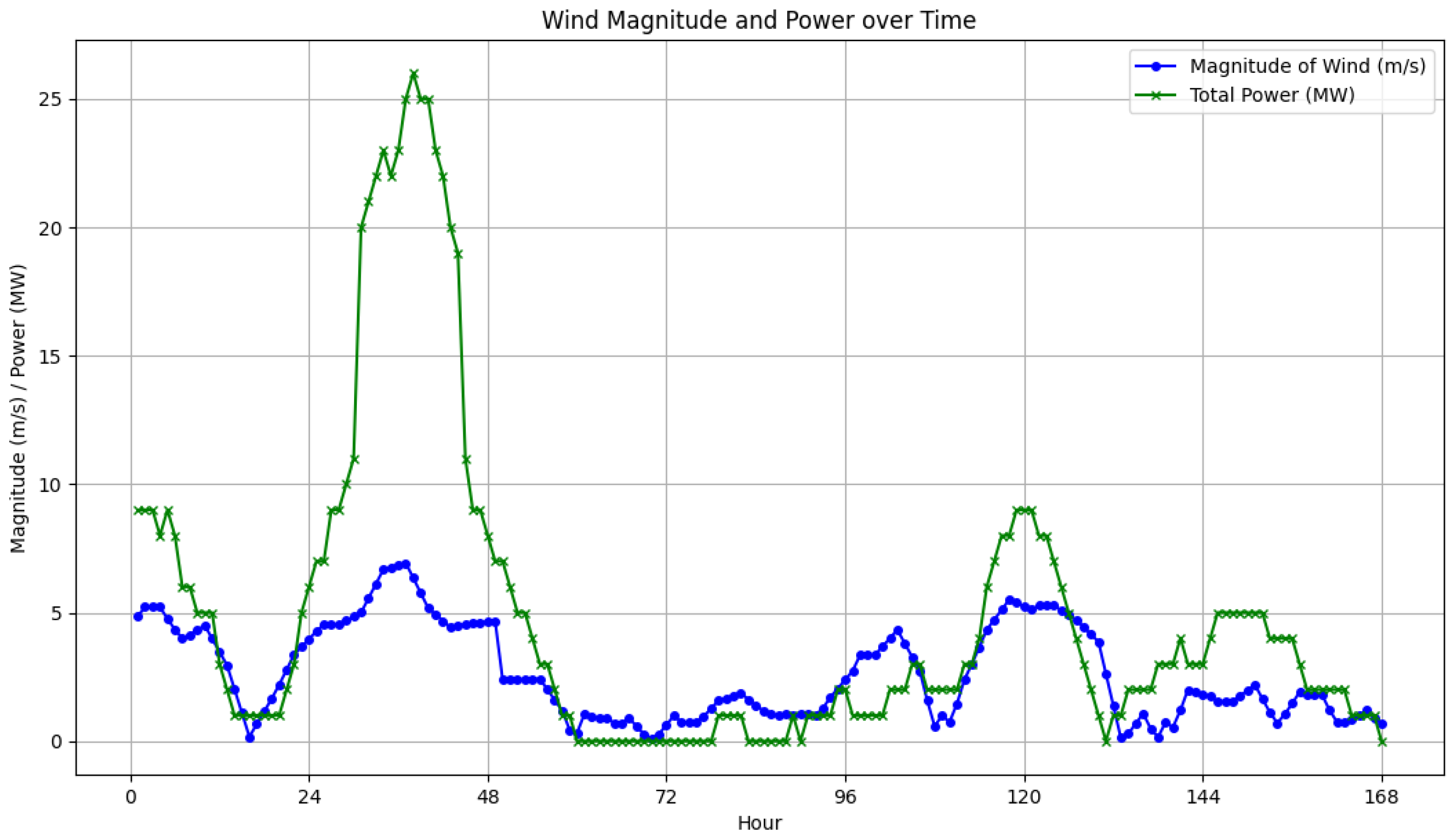
Also, information on the total production power of wind power plants is available hourly for the entire region. To enhance the clarity of the data presentation, Figure 1 illustrates the magnitude of wind speeds recorded at measurement point 8, along with the total power production for the entire zone over one week from 21 January to 27 January 2022 (168 h).

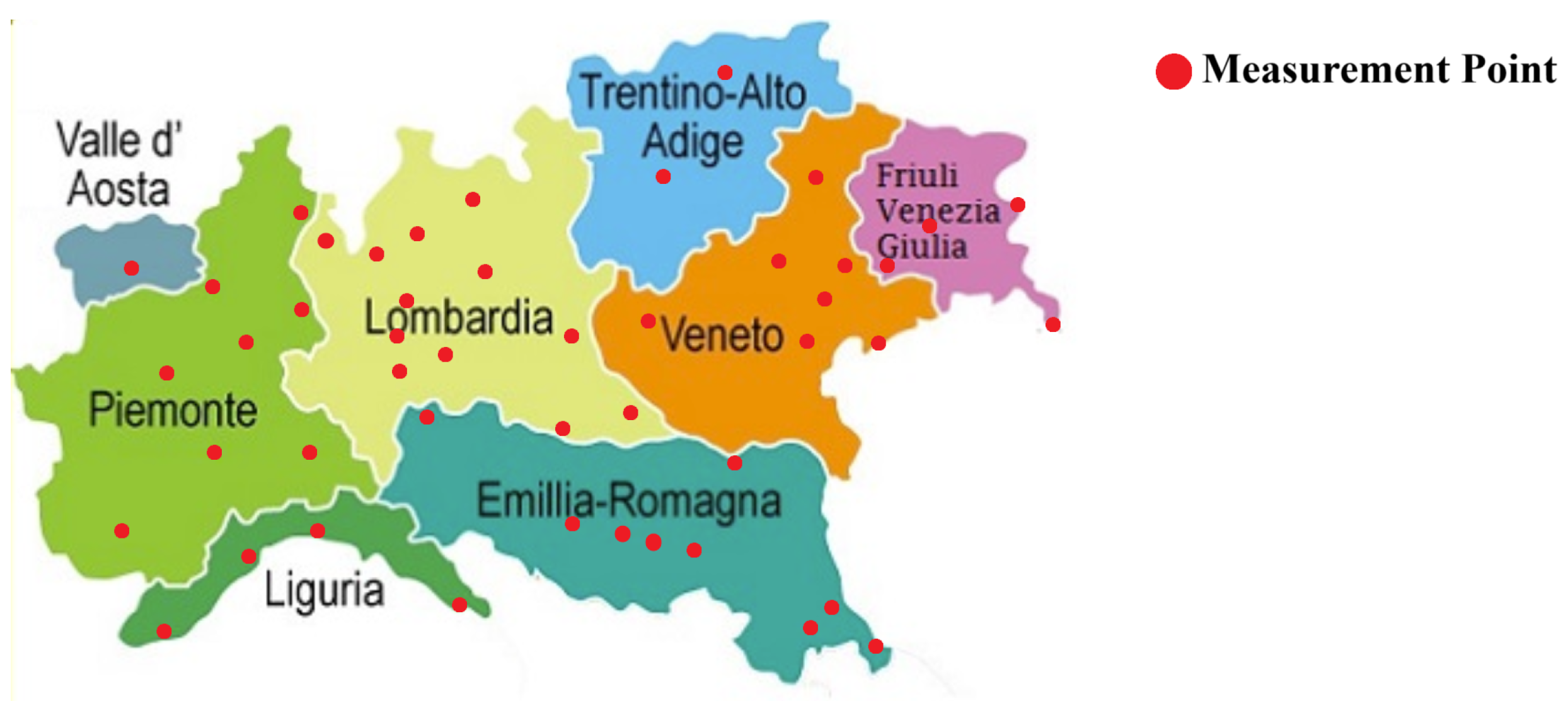
However, the exact distribution of the wind power plants across the region and their specific locations remain unclear. This lack of detailed spatial information presents a challenge for accurately predicting power production. Figure 2 illustrates the study zone and the locations of the meteorological stations.

The complexity of predicting the total production power under these conditions requires a more nuanced approach. Unlike scenarios where predictions are made for individual power plants using their specific meteorological data, this case demands sophisticated analysis and the application of various ML methods. Emphasizing feature selection is crucial to improve the accuracy of predictions, given the limited information on the spatial distribution of the power plants.

4. Machine-Learning Method Selection

In recent years, the application of ML techniques in predicting the production power of wind power plants has garnered significant attention. Based on the comprehensive review provided in [31], five techniques have been identified as particularly prominent and effective: LSTM networks, ELM, ANN, CNN, and SVM. These methods have been extensively utilized due to their ability to handle complex and nonlinear relationships in data, making them suitable for the intricate task of wind power prediction. In this section, each of these methods will be explored in detail, and then they will be utilized for forecasting wind power production using wind speed as a feature. This study will demonstrate which method performs best for this specific case study.

4.1. Description of the Considered Methods

LSTM: LSTM networks are a type of recurrent neural networks that are particularly well-suited for time-series forecasting due to their ability to capture long-term dependencies in sequential data. This method was proposed in 1997 [32]. LSTM networks are designed to overcome the vanishing gradient problem encountered in traditional recurrent neural networks by incorporating memory cells that can maintain information over long periods. The key components of an LSTM cell include the input gate, forget gate, and output gate, which regulate the flow of information. The cell state $C_t$ and the hidden state $h_t$ are updated using the following equations:

$$f_t=\sigma (W_f·[h_{t-1},x_t]+b_f)$$

(1)

$$i_t=\sigma (W_i·[h_{t-1},x_t]+b_i)$$

(2)

$$o_t=\sigma (W_o·[h_{t-1},x_t]+b_o)$$

(3)

$${\tilde{C}}_t=tanh(W_C·[h_{t-1},x_t]+b_C)$$

(4)

$$C_t=f_t\ast C_{t-1}+i_t\ast {\tilde{C}}_t$$

(5)

$$h_t=o_t\ast tanh\left(C_t\right)$$

(6)

where $f_t$, $i_t$, and $o_t$ represent the forget, input, and output gates, respectively; $\sigma$ is the sigmoid function; and tanh is the hyperbolic tangent function. The matrices $W_f,W_i,W_o,$ and $W_C$ are weights and $b_f,b_i,b_o,$ and $b_C$ are biases.

In the context of wind power plant forecasting, LSTM networks have been shown to effectively predict power output by leveraging historical wind speed data. Based on [31], 27% of the papers utilize this method for predicting the production power of wind power plants.

ANNs: ANNs are computational models inspired by the human brain, capable of recognizing complex patterns and relationships in data. An ANN consists of interconnected layers of neurons, including an input layer, one or more hidden layers, and an output layer. Each neuron applies a weighted sum of its inputs, passes the result through an activation function, and transmits the output to the neurons in the next layer. The training process involves adjusting the weights to minimize the error between the predicted and actual outputs using backpropagation.

The output of a single neuron can be described by the following equation:

$$y=\varphi \left(\sum _{i=1}^n{w}_i{x}_i+b\right)$$

(7)

where y is the neuron’s output, $\varphi$ is the activation function (such as sigmoid, ReLU, or tanh), $x_i$ are the inputs, $w_i$ are the weights, and b is the bias.

ANNs have proven effective in capturing the nonlinear relationships between wind speed and power output for wind power plant forecasting. As mentioned in [31], 17% of the articles focused on predicting the production power of wind power plants have employed this method. This significant usage underscores the effectiveness and reliability of this method in forecasting wind power production.

SVMs: SVMs are supervised learning models used for classification and regression tasks. SVMs are particularly effective for high-dimensional spaces and are known for their ability to model complex, nonlinear relationships using kernel functions. The basic idea of an SVM is to find the hyperplane that best separates the data into different classes or, in the case of regression, to find the optimal margin that minimizes the prediction error.

For regression tasks, SVMs use a method known as Support Vector Regression (SVR). The objective of SVR is to find a function $f\left(x\right)$ that deviates from the actual target values by a value no greater than $ϵ$ for all training data points while being as flat as possible. This is expressed mathematically as:

$$f\left(x\right)=\sum _{i=1}^n({\alpha }_i-{\alpha }_i^{\ast })K(x_i,x)+b$$

(8)

where ${\alpha }_i$ and ${\alpha }_i^{\ast }$ are the Lagrange multipliers, $K(x_i,x)$ is the kernel function, and b is the bias term. Common kernel functions include linear, polynomial, and radial basis function kernels.

SVMs have shown promise for wind power plant forecasting due to their ability to handle nonlinear and high-dimensional data efficiently. This method is utilized in 16% of articles within the field of wind power plant energy forecasting, highlighting its high capability in accurately predicting power production [31].

ELM: ELMs are a type of single-layer feedforward neural network that offer fast learning speeds and good generalization performance. Unlike traditional neural networks, ELMs randomly assign the weights between the input and hidden layers and only train the weights between the hidden and output layers, resulting in a much faster training process. This method eliminates the need for iterative tuning of the weights, making it computationally efficient.

The following equation can describe the output of an ELM:

$$H\beta =T$$

(9)

where H is the hidden layer output matrix, $\beta$ is the weight matrix between the hidden and output layers, and T is the target output matrix. The hidden layer output matrix H is calculated as:

$$h_{ij}=g(w_i·x_j+b_i)$$

(10)

where g is the activation function, $w_i$ are the input weights, $x_j$ are the input data, and $b_i$ are the biases.

Due to their ability to efficiently manage large datasets and accurately model complex relationships between wind speed and power output, ELMs have demonstrated considerable potential for wind power plant forecasting. According to the results of [31], this method has been utilized in 13% of the articles related to wind power production forecasting, indicating its significant presence in the field.

CNNs: CNNs are a specialized type of neural network primarily used for processing grid-like data structures, such as images. However, they have also been effectively applied in time-series forecasting, including predicting wind power production. CNNs are composed of convolutional layers, pooling layers, and fully connected layers. The convolutional layers apply convolution operations to the input data using filters (kernels) to extract local features, while the pooling layers reduce the spatial dimensions, making the computation more efficient and robust to variations.

The operation of a convolutional layer can be expressed as:

$$(X\ast W)[i,j]=\sum _m\sum _{n}X[i+m,j+n]·W[m,n]+b$$

(11)

where X is the input matrix, W is the filter (kernel) matrix, and b is the bias. The output of this operation, called the feature map, highlights the presence of specific patterns in the input data.

CNNs can capture spatial and temporal correlations in wind speed data. By applying convolutional layers to time-series data, CNNs can identify relevant patterns that are predictive of wind power output. This capability has led to CNNs being utilized in 11% of the articles related to forecasting wind power plant production [31].

As is evident, approximately 84% of the articles in the field of forecasting wind power plant production have utilized these five methods. Consequently, this study employs these methods to predict the specific case study and identify the most efficient one. For the case study, wind speed and production power data are available for 14 months, from 20 January 2022 to 20 March 2023. Initially, the parameters of these models will be adjusted using data from the first two months, i.e., 20 January 2022 to 20 March 2023. Subsequently, predictions will be made for the data from the following year to determine the best method.

4.2. Hyperparameter Tuning

Hyperparameter tuning is a critical step in the development of effective ML models, significantly influencing their performance and ability to generalize to new data. Adjusting hyperparameters such as learning rate, batch size, and the number of layers or neurons in a network is essential for optimizing the model’s accuracy and efficiency. According to [33], systematic hyperparameter tuning can substantially improve model performance. The study [34] emphasizes that effective hyperparameter optimization is crucial for enabling the model to capture complex patterns in the data while avoiding both overfitting and underfitting, which is essential for making accurate predictions.

Moreover, Bergstra and Bengio [33] emphasized the effectiveness of automated hyperparameter search methods, such as grid search and random search. These methods systematically explore the hyperparameter space and often outperform manual tuning by efficiently identifying the optimal settings [35]. Proper tuning is particularly important in applications like wind power forecasting, where accurate predictions can enhance the efficiency and reliability of power generation systems. Therefore, meticulous tuning of hyperparameters is indispensable for achieving optimal results in predictive modeling tasks. Cross-validation is a crucial technique employed alongside hyperparameter tuning to evaluate a model’s generalization performance and mitigate overfitting. By dividing the dataset into several subsets, known as folds, cross-validation facilitates training the model on one subset while assessing its performance on a separate subset. This iterative process is conducted across all folds, with the average performance metric providing an estimate of the model’s overall generalization capability. K-fold cross-validation, a widely used variant, partitions the data into K equal folds, where each fold is used as the validation set once, and the remaining folds constitute the training data [36].

Implementing cross-validation offers a more robust performance estimation than a single train–test split. By integrating cross-validation during hyperparameter tuning, one can identify hyperparameter values that yield the best model performance on unseen data, thereby enhancing the reliability and accuracy of predictions, such as in solar PV power forecasting [37]. To tune hyperparameters, data from the first two months (20 January 2022, to 20 March 2022) was utilized, implementing a thorough hyperparameter tuning approach involving grid search and five-fold cross-validation. The data are divided into five folds, and the training and validation process is repeated five times. In each iteration, four folds are utilized as training data while one fold serves as the test data. The goal of the grid search was to find the optimal hyperparameters by minimizing the Normalized Root Mean Squared Error (NRMSE), which is derived from the Root Mean Squared Error (RMSE) using the following formula [38]:

$$\mathrm{NRMSE}={\displaystyle \frac{\mathrm{RMSE}}{\mathrm{Range}}}={\displaystyle \frac{\sqrt{\frac{1}{n}{\sum }_{i=1}^n{(y_{\mathrm{true},i}-y_{\mathrm{pred},i})}^2}}{y_{\max }-y_{\min }}}$$

(12)

where:

• n represents the number of samples
• $y_{\mathrm{true},i}$ is the actual value of the target variable for sample i
• $y_{\mathrm{pred},i}$ is the predicted value of the target variable for sample i
• RMSE stands for Root Mean Squared Error
• Range denotes the range of the target variable ($y_{\max }-y_{\min }$), where $y_{\max }$ and $y_{\min }$ are the maximum and minimum values of the true target variable, respectively.

The outcomes of the hyperparameter adjustments are summarized in

Table 1. Summary of hyperparameters for LSTM.

Hyperparameter	Value
LSTM Layer Units	First LSTM layer: 150
	Second LSTM layer: 200
Dropout Rates	After first LSTM layer: 0.3
	After second LSTM layer: 0.3
	After Dense layer: 0.2
Dense Layer Units	First Dense layer: 200
	Output Dense layer: 1
Optimizer	Adam
Learning Rate	0.001
Early Stopping	Monitor: val_loss
	Patience: 10 epochs
Training Parameters	Epochs: 100
	Batch size: 32

,

Table 2. Summary of hyperparameters for ANN.

Hyperparameter	Value
Hidden Layer Sizes	1 hidden layer with 100 neurons
Activation Function	relu
Solver	sgd
Alpha	0.0001
Learning Rate	constant
Initial Learning Rate	0.001
Maximum Iterations	500
Random State	42

,

Table 3. Summary of hyperparameters for SVM.

Hyperparameter	Value
Kernel	rbf
C	1
Epsilon	0.1

,

Table 4. Summary of hyperparameters for CNN.

Hyperparameter	Value
Filters	128
Kernel Size	4
Activation	relu
Pool Size	2
Dense Units	100
Dropout Rate	0.3
Epochs	100
Batch Size	64
Monitor	val_loss
Patience	10
Restore Best Weights	True

and

Table 5. Summary of hyperparameters for ELM.

Hyperparameter	Values
n_neurons	100
Activation	sigm

.

4.3. Comparison of Machine-Learning Methods without Feature Selection

In this section, the focus is on forecasting the production power in the studied area using the introduced ML methods and the optimized hyperparameter settings to identify the best model for this case study.

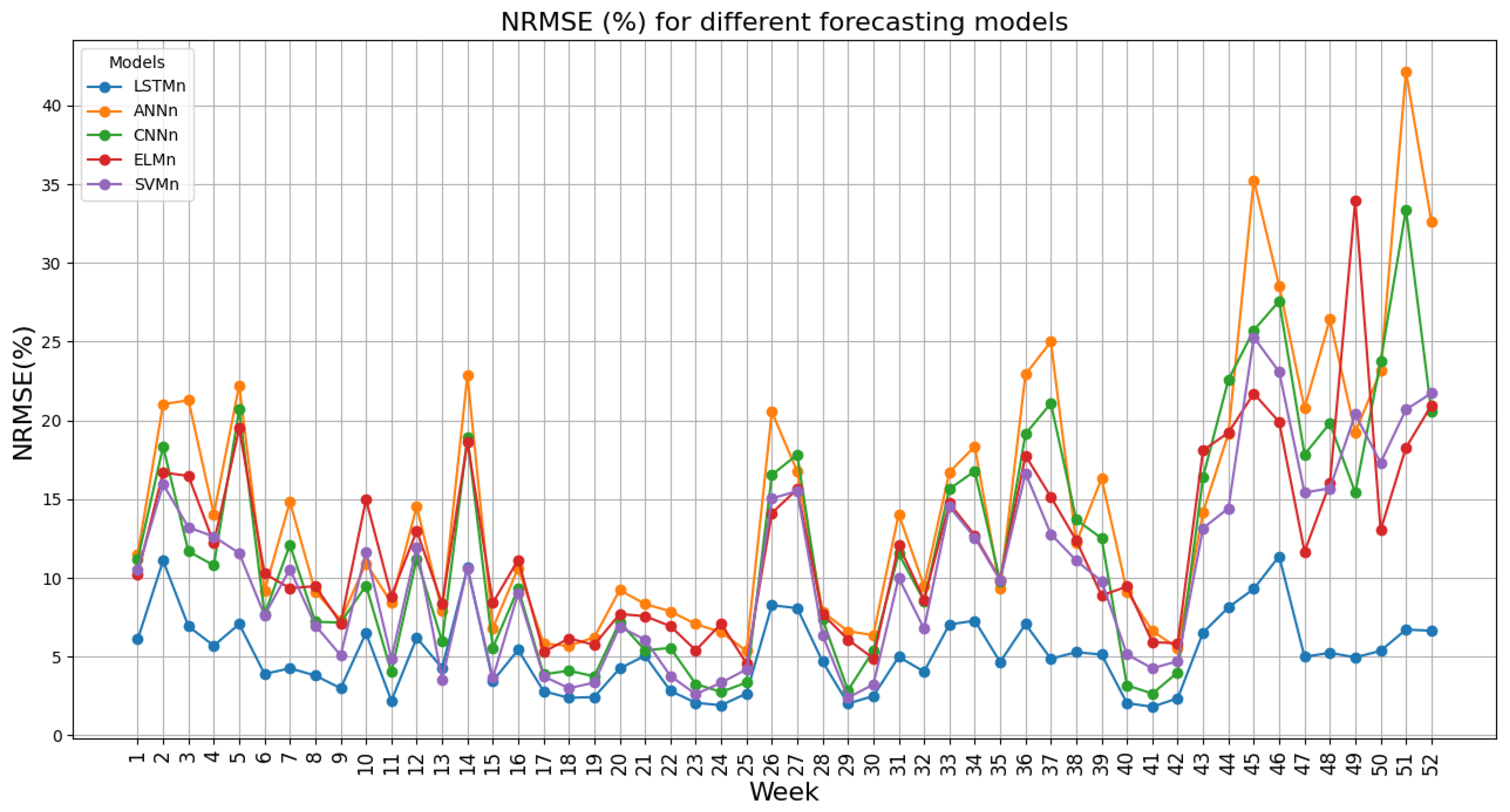
The prediction scenario is as follows: Initially, two months of data from 20 January 2022 to 20 March 2022 are used as training data, and the week after this period is used as test data. Subsequently, all the data are shifted forward by one week, and this process is repeated for 52 weeks. This approach ensures one year of forecasting, thereby enhancing the comprehensiveness of the method and results. The simulation results spanning 52 weeks are presented in Figure 3. The figure includes the NRMSE expressed as a percentage.

Table 6. Comparison of model performance.

Model	Overall NRMSE (%)
LSTM	5.69
CNN	14.09
ELM	13.31
ANN	16.87
SVM	13.79

provides an overview of the overall NRMSE for all five methods.

The results from Figure 3 and Table 6 clearly demonstrate that LSTM outperforms other methods in terms of efficiency in this case study. Therefore, this method is chosen as the best method for forecasting the production capacity of the studied area, and in the rest of the research the analyses are done only for this method.

5. Feature-Selection Methods

5.1. Define Feature-Selection Methods

Feature selection is a crucial step in developing accurate wind power forecasting models for this case study. Given the lack of information about the locations of wind power plants and the presence of 47 different wind measuring points—many of which may be unrelated to the wind power plants and could introduce noise into the forecasting process—feature selection becomes essential. This process involves selecting a subset of relevant features from a larger set of potential predictors to enhance the model’s accuracy and interpretability while reducing its complexity and computational cost.

This section provides an overview of the feature-selection methods used in wind power forecasting, highlighting key techniques within the filter methods category. Subsequently, several of these methods are applied to the problem to identify the most effective one.

1. Filter Methods: Filter methods evaluate the relevance of features independently of the chosen learning algorithm. Examples include the Pearson correlation coefficient, which is used to measure the linear relationship between features and the target variable (e.g., wind power output), as demonstrated in related works [39]. The Spearman rank correlation coefficient captures monotonic relationships between features and target variables in wind forecasting studies [23]. The Chi-squared test and Fisher score evaluate the independence of categorical features from the target variable [40]. Mutual information measures statistical dependence between variables, effectively capturing nonlinear relationships, and is widely used in wind power forecasting [41]. Relief-F estimates feature quality based on their ability to distinguish between instances of different classes, effectively handling noisy and irrelevant features [42]. Variance threshold selects features with significant variance, filtering out low-variance predictors.

2. Wrapper Methods: Wrapper methods use the learning algorithm to evaluate feature subsets, often improving performance but with higher computational costs. Recursive feature elimination iteratively removes the least impactful features to enhance prediction accuracy in wind forecasting. Sequential forward selection adds features one by one, while sequential backward elimination removes the least significant features, both optimizing model performance [43]. Genetic algorithms mimic natural selection to explore and exploit feature subsets and are widely applied in wind power forecasting [44].

3. Embedded Methods: Embedded methods integrate feature selection with model training, offering a more efficient approach. L1 Regularization (Lasso) adds a penalty term to shrink irrelevant feature coefficients to zero, effectively eliminating them, and has been useful in identifying key predictors in wind power forecasting [45]. L2 Regularization (Ridge) uses a different penalty term to handle multicollinearity, stabilizing models with highly correlated predictors [46]. Decision-tree-based methods, like random forests and gradient boosting trees, perform feature selection by ranking feature importance based on split criteria and have been widely applied in wind forecasting [47].

Filter methods offer distinct advantages over wrapper and embedded methods in feature selection. They are computationally efficient and scalable, making them particularly suitable for handling large datasets with numerous features [48]. Unlike wrapper methods, which involve iterative model training and are computationally demanding, filter methods evaluate feature relevance independently of the learning algorithm, thereby reducing computational overhead and avoiding overfitting concerns during feature selection [49]. Additionally, filter methods, such as correlation-based approaches, assess each feature’s importance in isolation, making them transparent and interpretable in identifying relevant features without being influenced by multicollinearity [50]. These characteristics underline the practical advantages of filter methods in scenarios where computational efficiency, scalability, and straightforward interpretability are crucial considerations. In this study, four distinct filter methods—Pearson correlation, Spearman correlation, Chi-squared test with Fisher score, and mutual information—were compared to determine which method most enhances prediction accuracy. These methods were selected for their capability to effectively handle high-dimensional data without relying on prior knowledge of feature relationships to power output.

5.2. Choosing Feature-Selection Method

As mentioned earlier, filter methods select features only based on the data, focusing on statistical relationships between each feature and the output. Since feature selection is independent of the learning algorithm, training is not required to assign feature scores. However, selecting the most relevant features requires setting a threshold based on their scores, and the method’s performance must be evaluated for different threshold values to determine the optimal one.

The following section introduces the filtering methods in more detail and identifies the most effective features.

5.2.1. Pearson Correlation

The Pearson correlation coefficient, often denoted as $\rho$, is a measure of the linear relationship between two variables, typically used to assess the strength and direction of association between them. It quantifies how much a change in one variable is associated with a change in another variable. Here is the formula for calculating the Pearson correlation coefficient between two variables X and Y:

$${\rho }_{X,Y}={\displaystyle \frac{\mathrm{cov}(X,Y)}{{\sigma }_X{\sigma }_Y}}$$

(13)

where:

${\rho }_{X,Y}$ is the Pearson correlation coefficient between variables X and Y.

$\mathrm{cov}(X,Y)$ is the covariance of X and Y.

${\sigma }_X$ and ${\sigma }_Y$ are the standard deviations of X and Y, respectively.

The covariance $\mathrm{cov}(X,Y)$ is calculated as:

$$\mathrm{cov}(X,Y)={\displaystyle \frac{1}{n}}\sum _{i=1}^n(X_i-\overline{X})(Y_i-\overline{Y})$$

(14)

where $\overline{X}$ and $\overline{Y}$ are the means of X and Y, respectively, and n is the number of data points.

The Pearson correlation coefficient ${\rho }_{X,Y}$ ranges from −1 to 1:

-

${\rho }_{X,Y}=1$: Perfect positive linear relationship.

-

${\rho }_{X,Y}=-1$: Perfect negative linear relationship.

-

${\rho }_{X,Y}=0$: No linear relationship (variables are not linearly correlated).

In feature selection, Pearson correlation can be used to measure the linear relationship between each feature and the target variable (such as wind power output). Features with high absolute correlation coefficients are typically considered more relevant for prediction tasks. However, it is important to note that Pearson correlation assumes a linear relationship and may not capture nonlinear associations between variables [39].

To employ this feature-selection method, data from 20 January 2022 to 20 March 2022 was analyzed to assess the importance of features for power forecasting. Initially, the ranking of feature importance was determined; however, establishing an appropriate threshold for filtering the most effective features remained ambiguous. To address this, feature scores were divided into equal intervals. For each interval value, cross-validation was conducted using five folds and an 80:20 training-to-test ratio. Eventually, the optimal threshold that minimized the average NRMSE was identified. Figure 4 illustrates the detailed process of selecting the best threshold.

The figure shows that the lowest NRMSE value is 20.7352%, achieved by selecting features with a threshold greater than 0.21.

5.2.2. Spearman Correlation

The Spearman correlation coefficient ($\rho$) is a statistical measure that evaluates the strength and direction of the monotonic relationship between two variables. It is calculated using the formula:

$$\rho =1-{\displaystyle \frac{6{\sum }_{i=1}^n{d}_i^2}{n(n^2-1)}}$$

(15)

where $d_i=R_{X,i}-R_{Y,i}$ represents the difference in ranks for each paired observation $(R_{X,i},R_{Y,i})$, n is the number of paired observations, and $R_{X,i}$ and $R_{Y,i}$ are the ranks of the i-th observation of variables X and Y, respectively.

To compute the Spearman correlation coefficient:

1.

Ranking: Assign ordinal ranks to each variable’s observations, from 1 (lowest) to n (highest).

2.

Calculate differences: Compute the difference $d_i$ for each pair of ranked observations.

3.

Square differences: Square each difference, $d_i$.

4.

Summation: Sum all squared differences, ${\sum }_{i=1}^n{d}_i^2$.

5.

Apply formula: Substitute the sum of squared differences into the formula to calculate $\rho$.

The resulting coefficient $\rho$ ranges from −1 to 1:

-

$\rho =1$ indicates a perfect positive monotonic relationship.

-

$\rho =-1$ indicates a perfect negative monotonic relationship.

-

$\rho =0$ indicates no monotonic relationship.

Spearman correlation is particularly useful in analyzing relationships between variables measured on ordinal scales or when assumptions of linearity and normality are not met. It provides a robust measure of association that is less sensitive to outliers compared to other correlation measures [50]. To determine the optimal threshold in this method, a process similar to that used with the Pearson method is followed. The outcome of this analysis is depicted in Figure 5.

The figure indicates that the lowest NRMSE value of 20.7135% is achieved when selecting features with a threshold greater than 0.4.

5.2.3. Mutual Information

Mutual information is a measure from information theory that quantifies the amount of information gained about one random variable through another. It is a crucial tool for understanding the dependency between variables, capturing the reduction in uncertainty about one variable given the knowledge of another. Formally, for two discrete random variables, X and Y, mutual information is defined as:

$$I(X;Y)=\sum _{x\in X}\sum _{y\in Y}p(x,y)log\left({\displaystyle \frac{p(x,y)}{p\left(x\right)p\left(y\right)}}\right)$$

(16)

where $p(x,y)$ is the joint probability distribution of X and Y and $p\left(x\right)$ and $p\left(y\right)$ are their marginal distributions. For continuous variables, the definition involves integrals. MI is non-negative and symmetric, meaning $I(X;Y)=I(Y;X)$, and equals zero if and only if the variables are independent [51]. The same procedure as used in the previous two methods is employed to determine the optimal threshold for selecting the most effective features. The result is illustrated in Figure 6.

The figure shows that the minimum NRMSE value of 21.5159% is obtained when features are selected with a threshold exceeding 0.195.

5.2.4. Chi-Squared Test and Fisher Score

The Chi-squared test is a statistical method used to examine the relationship between two categorical variables, determining if they are independent or associated. It involves comparing the observed frequencies in a contingency table to the expected frequencies, calculated under the assumption that the variables are independent. The test statistic is calculated using the formula:

$${\chi }^2=\sum {\displaystyle \frac{{(O_i-E_i)}^2}{E_i}}$$

(17)

where $O_i$ represents the observed frequency and $E_i$ represents the expected frequency. A significant Chi-squared statistic, indicated by a low p-value, suggests that the variables are not independent and that there is a relationship between them. This test is widely used in hypothesis testing to validate the independence of categorical data.

In contrast, the Fisher score is a feature-selection technique used in ML to identify the most relevant features for classification tasks. It measures the importance of a feature by calculating the ratio of the variance between different classes to the variance within the same class, thereby highlighting features that best distinguish between classes. The formula for the Fisher Score is [52]:

$$\mathrm{Fisher}\mathrm{Score}\left(j\right)={\displaystyle \frac{{\sum }_{c=1}^C{n}_c{({\mu }_{j,c}-{\mu }_j)}^2}{{\sum }_{c=1}^C{n}_c{\sigma }_{j,c}^2}}$$

(18)

where j is the feature index, C is the number of classes, $n_c$ is the number of samples in class c, ${\mu }_{j,c}$ is the mean of the feature j in class c, ${\mu }_j$ is the overall mean of the feature j, and ${\sigma }_{j,c}$ is the standard deviation of the feature j in class c. A higher Fisher score indicates a feature with greater discriminative power. To identify the most effective features, two indicators are used simultaneously to measure feature quality. The features are divided into 100 parts based on both indicators. Any feature that meets the criteria for at least one of the indicators is included in the final table. The result is shown in Figure 7.

The figure indicates that the minimum NRMSE value of 21.0631% is achieved when features are selected with a threshold greater than 85.

Thus, by identifying the optimal threshold for each of the four methods, the most effective features were selected according to each method’s criteria.

6. Results and Discussion

In this section, the features selected by each feature-selection method are utilized to forecast production capacity in the region. The results from each method are compared to evaluate their effectiveness.

For forecasting, two months of data from 20 January 2022 to 20 March 2022 are used as the training set, and the subsequent week serves as the test set. After each prediction, all the data are shifted by one week, and the prediction process is repeated. This procedure is carried out for 52 weeks to cover the entire year, allowing us to assess the method’s effectiveness with a high degree of certainty. As previously mentioned, the data have an hourly granularity.

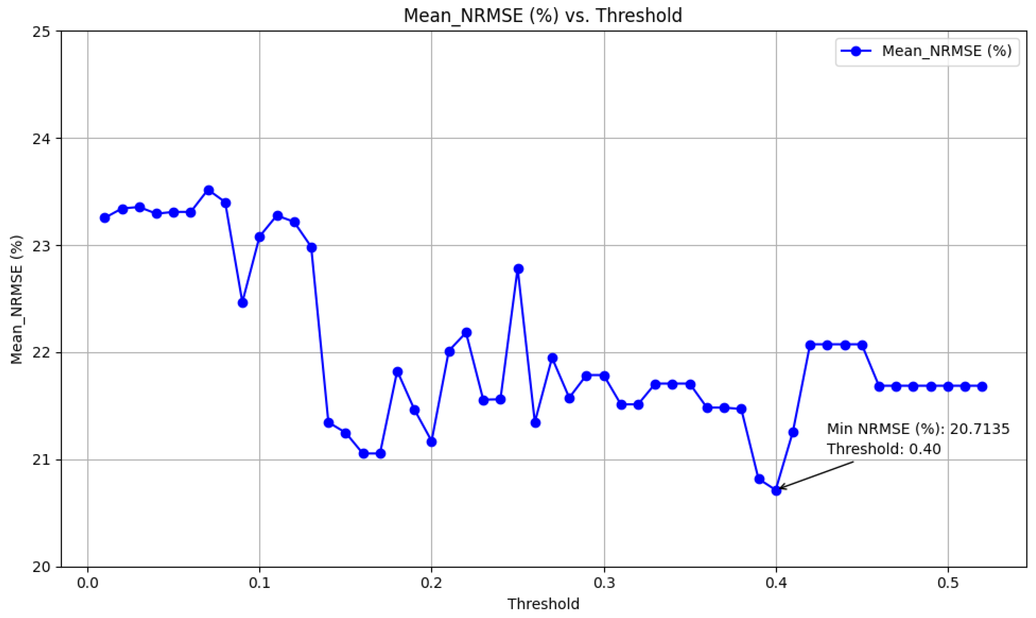
6.1. Forecasting Using Selected Features by the Pearson Method

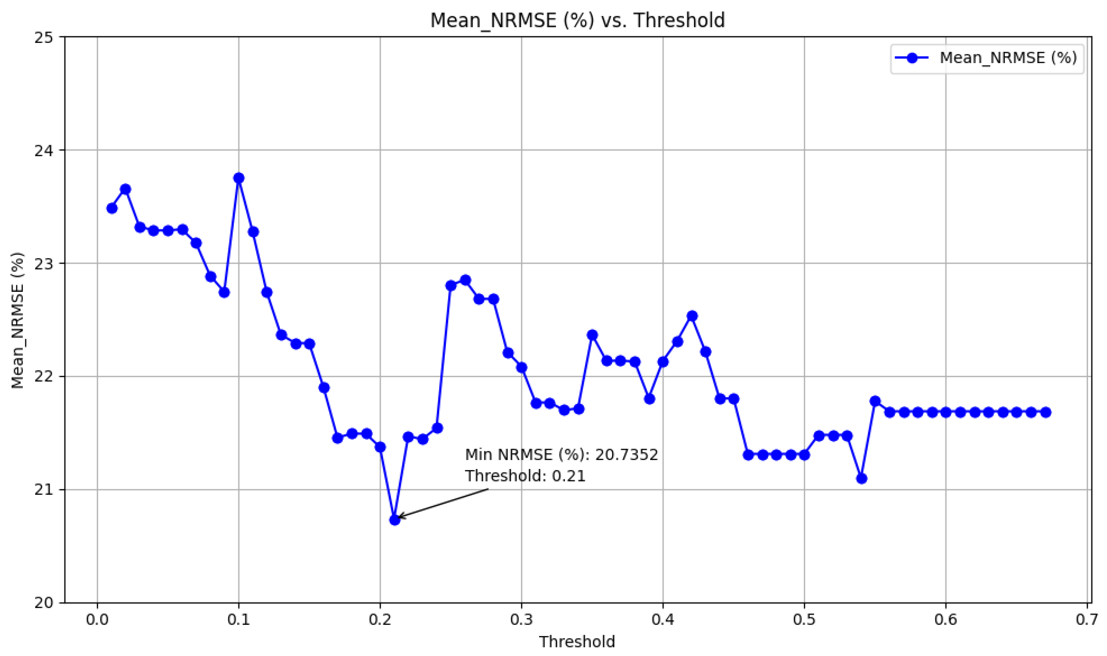
By applying the Pearson method with a threshold of 0.21, features that met this criterion were selected. From the 94 available features, 48 features were identified as relevant. These selected features are listed in

Table 7. Selected features with Pearson method.

Selected Feature
ugrd_10m1	ugrd_10m16	ugrd_10m36	vgrd_10m5	vgrd_10m20	vgrd_10m36
ugrd_10m3	ugrd_10m17	ugrd_10m37	vgrd_10m6	vgrd_10m22	vgrd_10m37
ugrd_10m4	ugrd_10m18	ugrd_10m38	vgrd_10m7	vgrd_10m23	vgrd_10m38
ugrd_10m6	ugrd_10m19	ugrd_10m39	vgrd_10m8	vgrd_10m24	vgrd_10m39
ugrd_10m7	ugrd_10m20	ugrd_10m40	vgrd_10m11	vgrd_10m27	vgrd_10m40
ugrd_10m8	ugrd_10m22	ugrd_10m44	vgrd_10m16	vgrd_10m28	vgrd_10m41
ugrd_10m13	ugrd_10m23	ugrd_10m45	vgrd_10m17	vgrd_10m30	vgrd_10m42
ugrd_10m15	ugrd_10m27	vgrd_10m3	vgrd_10m19	vgrd_10m33	vgrd_10m45

. As a guide, ugrd_10m1 is related to the east–west wind speed at measurement point 1 and vgrd_10m3 is related to the north–south wind speed at measurement point 3.

Using wind speed data from these selected areas as features, regional power production was predicted. The results of these predictions demonstrate the impact of feature selection on predictive accuracy, showing a decrease in the NRMSE from 5.69% to 5% with the implementation of feature selection. Additionally, it provides insights into the operational efficiencies gained through feature selection, showcasing a significant reduction in the number of features employed for forecasting, from 94 to 48. Furthermore, the average elapsed time for one-week forecasting was notably reduced from 410.68 s to 348.96 s, reflecting improved computational efficiency under consistent conditions with the same computer.

The implementation of effective feature-selection strategies not only enhances predictive accuracy but also optimizes computational resources. By minimizing feature complexity, the forecasting model becomes more streamlined and efficient, facilitating quicker model updates and responsiveness in dynamic forecasting scenarios. This streamlined approach not only improves forecasting accuracy but also enhances overall operational efficiency, making the forecasting process more agile and resource-effective.

6.2. Forecasting Using Selected Features by the Spearman Method

By utilizing the Spearman method with a threshold of 0.4, features that satisfied this criterion were identified. Out of the 94 available features, 5 were deemed relevant. These selected features are presented in

Table 8. Selected features with Spearman method.

Selected Feature
ugrd_10m8
ugrd_10m20
vgrd_10m5
vgrd_10m8
vgrd_10m23

.

The implementation of the Spearman method illustrates the comparative impact of feature selection on predictive accuracy, showing a reduction in the NRMSE from 5.69% to 3.92% with feature selection. It also details the reduction in the number of features used for forecasting, decreasing from 94 to 5, as well as the average elapsed time for one-week forecasting, which decreased from 410.68 s to 235.06 s under identical conditions and using the same computer.

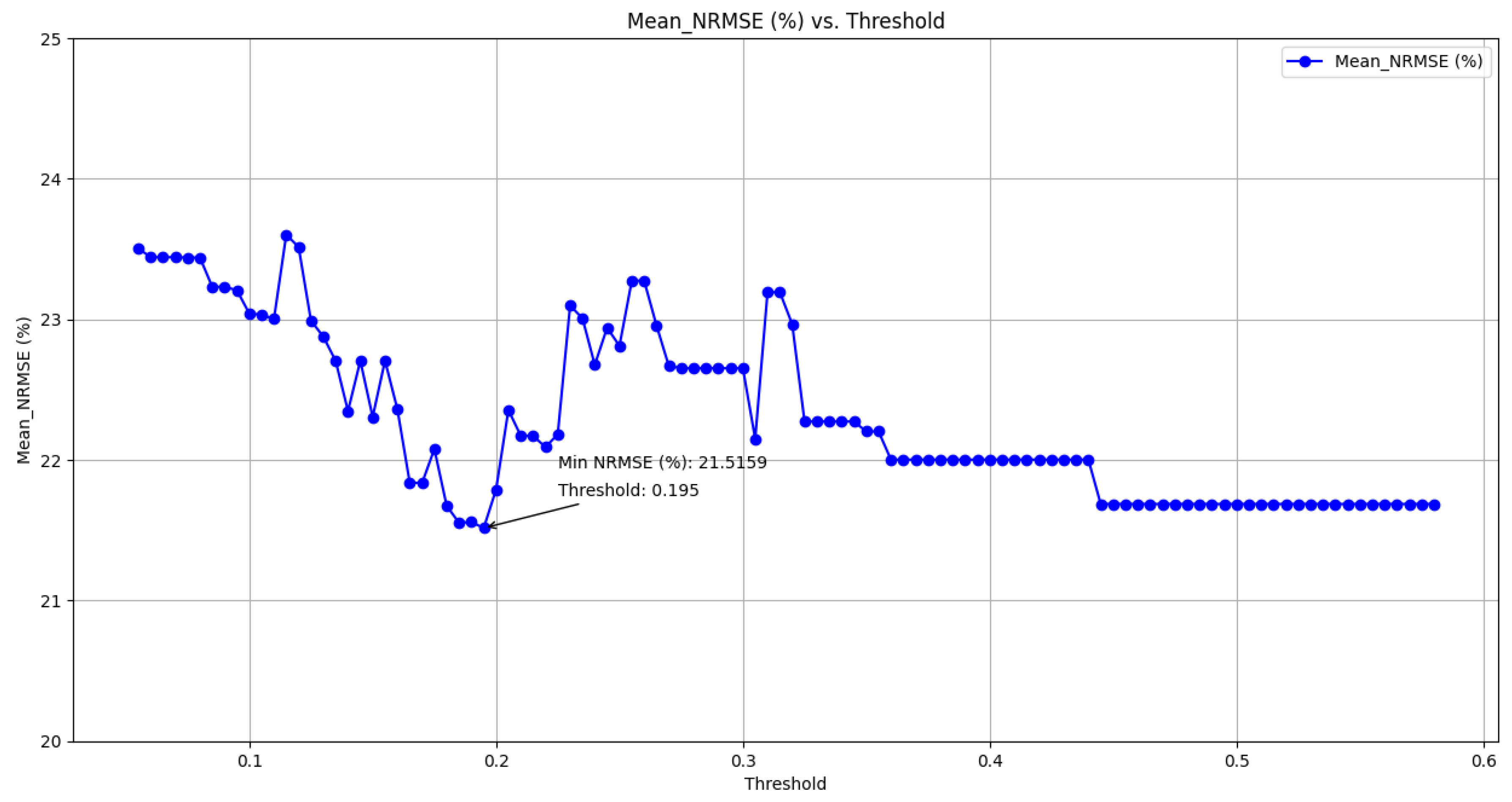
6.3. Forecasting Using Selected Features by the Mutual Information Method

By applying the mutual information method with a threshold of 0.195, features that met this criterion were selected. From the 94 available features, 42 were identified as relevant. These selected features are listed in

Table 9. Selected features with mutual information method.

Selected Feature
ugrd_10m3	ugrd_10m15	ugrd_10m23	ugrd_10m41	vgrd_10m3	vgrd_10m22
ugrd_10m4	ugrd_10m16	ugrd_10m30	ugrd_10m42	vgrd_10m5	vgrd_10m23
ugrd_10m6	ugrd_10m17	ugrd_10m34	ugrd_10m43	vgrd_10m6	vgrd_10m24
ugrd_10m8	ugrd_10m18	ugrd_10m36	ugrd_10m44	vgrd_10m7	vgrd_10m30
ugrd_10m10	ugrd_10m19	ugrd_10m37	ugrd_10m45	vgrd_10m8	vgrd_10m34
ugrd_10m11	ugrd_10m20	ugrd_10m39	ugrd_10m46	vgrd_10m11	vgrd_10m37
ugrd_10m13	ugrd_10m22	ugrd_10m40	ugrd_10m47	vgrd_10m19	vgrd_10m45

.

With the implementation of the mutual feature selection method, predictive accuracy is enhanced, reducing the NRMSE from 5.69% to 4.87%. Additionally, there is a substantial reduction in the number of features utilized for forecasting, declining from 94 to 42, alongside a noteworthy decrease in the average time required for one-week forecasting, dropping from 410.68 s to 311.94 s under identical conditions using the same computer.

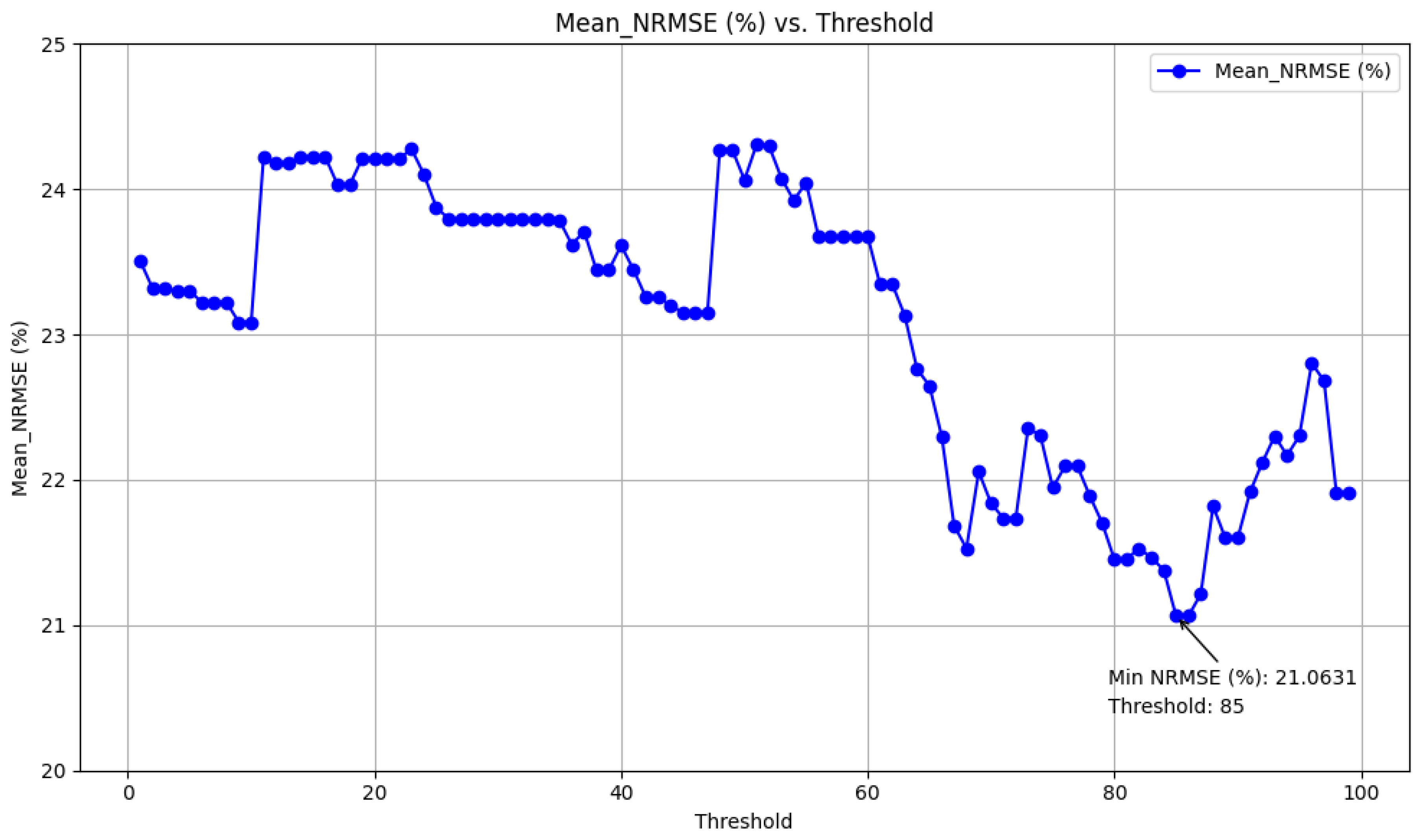
6.4. Forecasting Using Selected Features by the Chi-Squared Test and Fisher Score Method

By utilizing the Chi-squared test and Fisher score method with a threshold of 85, 19 relevant features were identified out of the 94 available. These features met the specified criterion and are detailed in

Table 10. Selected Features with Chi-squared test and Fisher score method.

Selected Feature
ugrd_10m3	ugrd_10m20	ugrd_10m42	vgrd_10m8
ugrd_10m4	ugrd_10m36	vgrd_10m3	vgrd_10m23
ugrd_10m8	ugrd_10m38	vgrd_10m5	vgrd_10m24
ugrd_10m13	ugrd_10m39	vgrd_10m6	vgrd_10m30
ugrd_10m16	ugrd_10m40	vgrd_10m7

.

Using this method leads to a decrease in the NRMSE from 5.69% to 4.43%. Additionally, it outlines the reduction in the number of features used for forecasting, which has dropped from 94 to 19, along with a reduction in the average time required for one-week forecasting, which has decreased from 410.68 s to 289.63 s, all under the same conditions and utilizing the same computer.

The results of all methods are presented in

Table 11. Comparison of feature-selection method results.

Feature Selection Method	Number of Selected Features	NRMSE (%)	Elapsed Time for Forecasting: Weekly Average (min)
Without feature selection	94	5.69	410.68
Pearson	48	5.00	348.96
Spearman	5	3.92	235.06
Mutual information	42	4.87	311.94
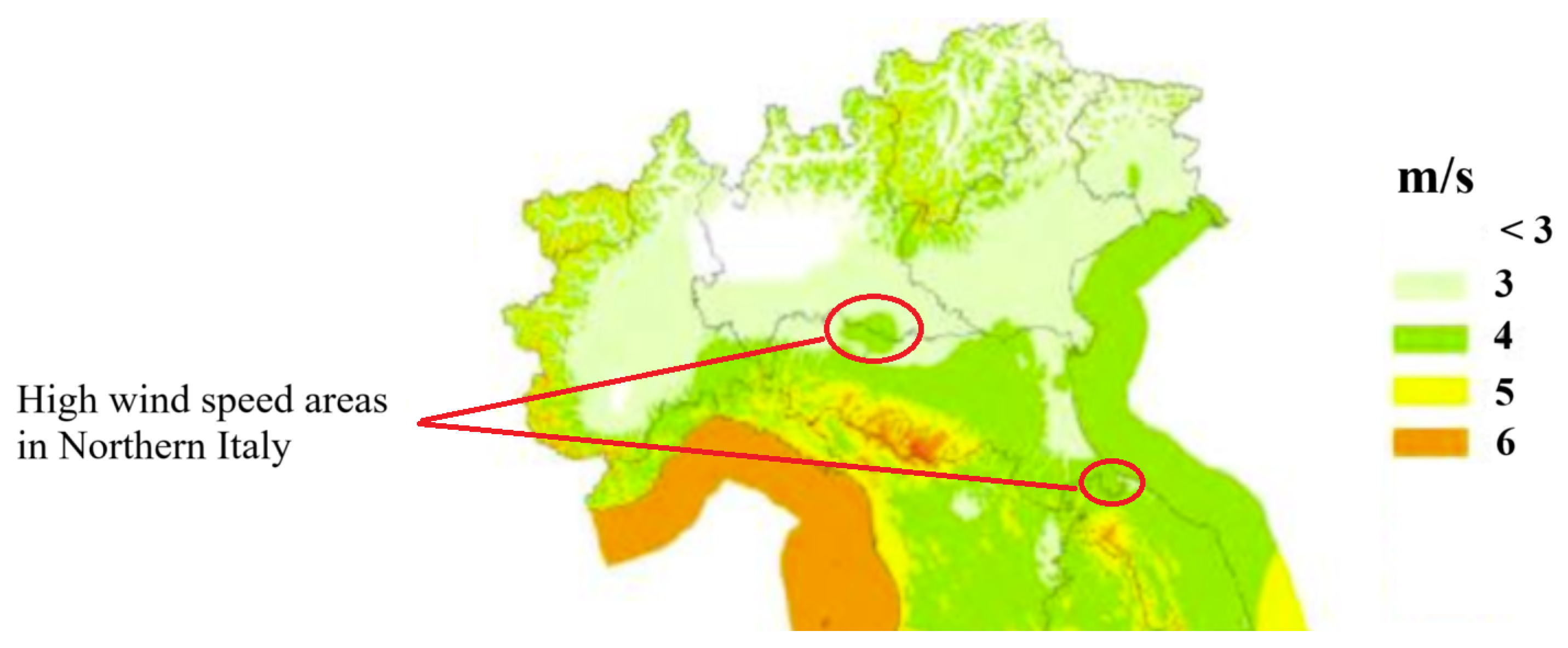
Chi-squared test and Fisher score	19	4.43	289.63

. Based on the results presented in this table, Spearman’s method demonstrates superior performance among the four evaluated methods. This approach not only selects the fewest number of features but also achieves the highest accuracy and the shortest prediction time for the study area. Consequently, Spearman’s method is highly efficient and effective in feature selection for this case study. The cities that have been selected as more effective cities with this method include Piacenza, Rimini, Cremona, and Mantova, whose locations are shown in Figure 8, which shows that the average wind speed (at 75 m) is high in the regions nearby those selected cities.

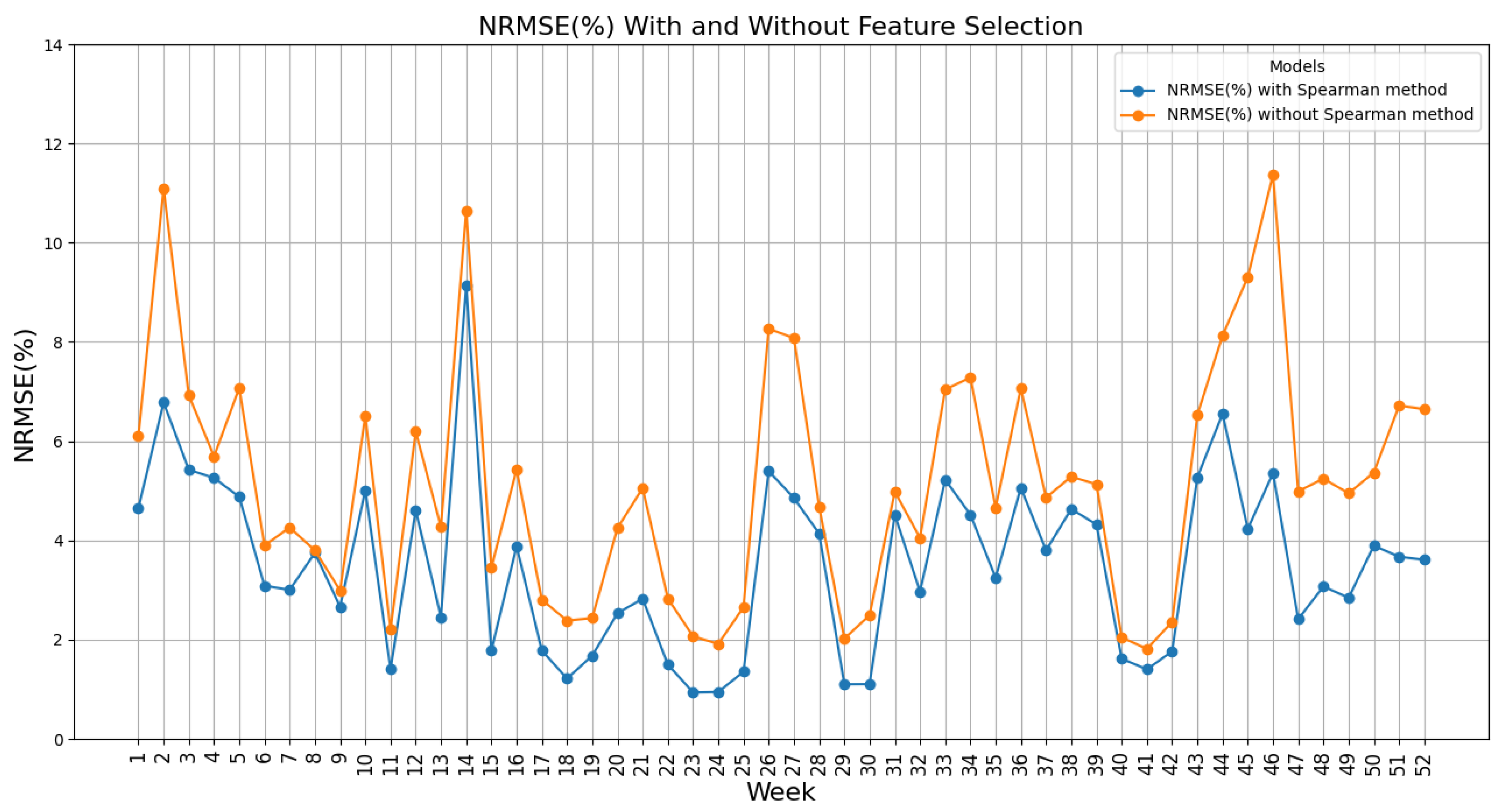
In Figure 9, NRMSE changes for weekly forecasts are presented, which shows that the range of changes by applying Spearman’s method is between 0.94 and 9.13%, while it was between 1.82% and 11.37% without applying this method.

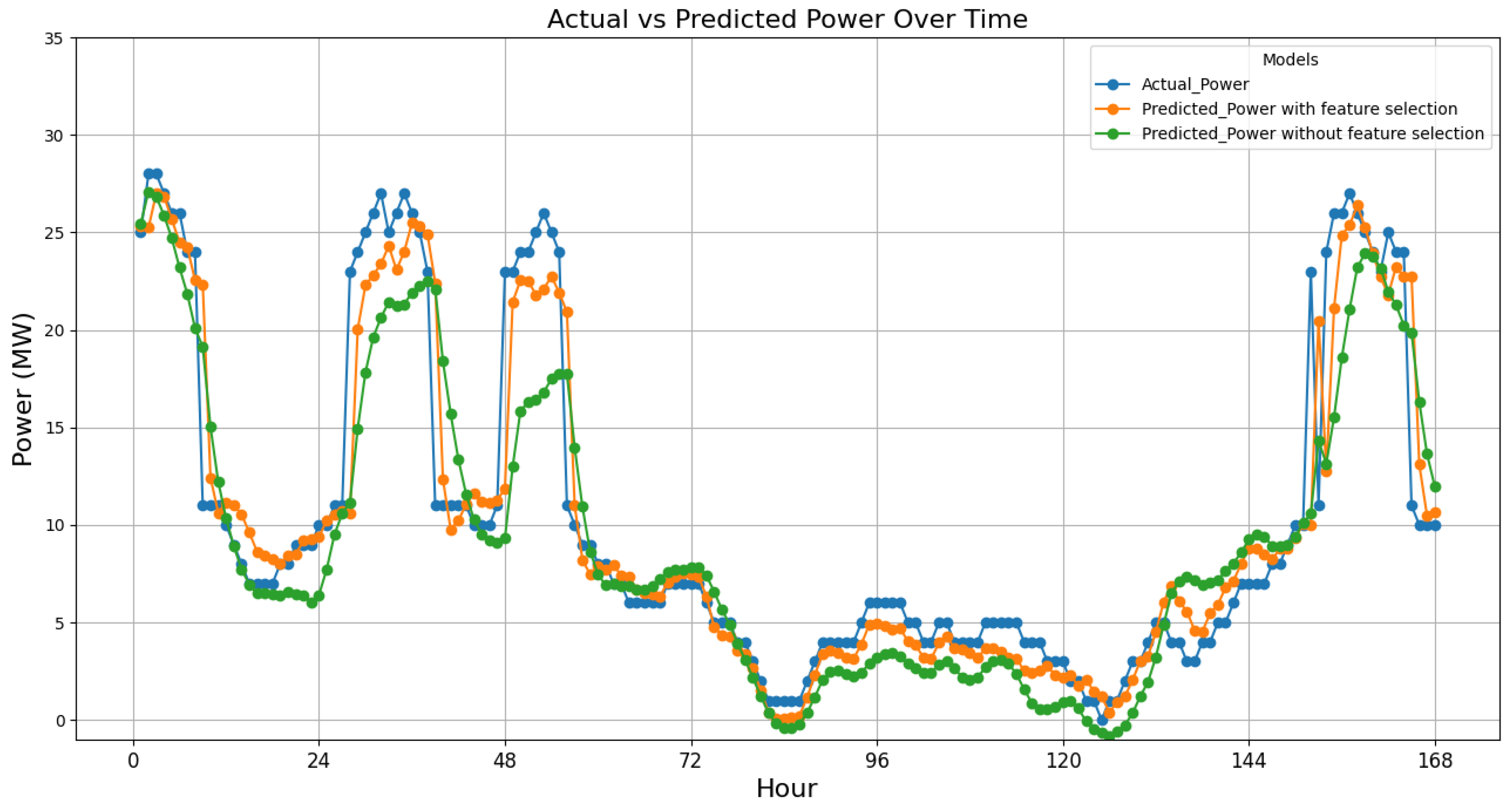
To demonstrate the effect of improving forecasting accuracy, the actual and forecasted data for a week from 21 March 2022 to 27 March 2022 (168 h) were compared in both cases: with and without feature selection. This comparison is illustrated in Figure 10.

Figure 10 clearly shows that incorporating effective feature selection has notably increased the prediction accuracy. Combining LSTM for forecasting and Spearman for feature selection yields the best overall performance for this study area and optimizes both performance and efficiency, making it the most advantageous combination among the tested methods. This efficiency is crucial for large datasets and real-time applications where quick and accurate predictions are necessary.

7. Conclusions

This study proposes an advanced methodology for enhancing regional wind power forecasting through the integration of machine-learning techniques and feature-selection methods. By systematically evaluating several machine-learning models—LSTM, ANN, SVM, CNN, and ELM—within the context of northern Italy, LSTM emerged as the most effective model for regional forecasting. Four distinct feature-selection methods (Pearson correlation, Spearman correlation, mutual information, and the Chi-squared test with Fisher score) were comprehensively investigated, demonstrating that Spearman correlation was the most efficient for this dataset.

The key advantage of regional evaluation, combined with feature-selection methods, compared to existing approaches in the research, lies in its ability to optimize prediction accuracy and computational efficiency in regions with sparse or incomplete data on individual wind farms. Most existing methods focus on plant-specific predictions, which require detailed data for each wind farm. However, in regions such as northern Italy, where such detailed data are often unavailable, regional forecasting offers a practical alternative. By utilizing meteorological data from multiple stations, corresponding to province capital cities, and applying effective feature-selection techniques, this approach not only improved forecasting accuracy but also significantly reduced the number of features required for reliable predictions. This leads to more efficient computations and makes the method highly scalable and applicable to other regions facing similar data constraints.

Furthermore, this study demonstrates that regional forecasting, when optimized with appropriate machine-learning models and feature selection, can bridge the gap between plant-specific forecasting and large-scale grid management. It provides a robust solution for grid operators to better manage renewable energy integration, balance supply and demand, and reduce uncertainty in power system operations. The reductions in NRMSE and computation time further highlight the practical contributions of this approach, enhancing both predictive performance and operational efficiency.

As a final remark, the Spearman correlation and the LSTM method proved to be the best-performing options for the northern region of Italy. However, if this approach were to be applied to another region, such as the south of Italy, the entire procedure of cross-validation and grid search would need to be repeated to identify the best ML method and the most effective feature-selection method, which may differ in that case. The mathematical justification that the Spearman correlation is the best choice for this test case is a numerical one, which is a common practice in the machine-learning community, where the best method is assessed by means of an exhaustive grid search based on a cross-validation approach.

In conclusion, the regional evaluation presented in this work offers substantial benefits over existing methods by addressing the challenges posed by limited plant-specific data, improving forecasting accuracy and optimizing computational resources. Future research could extend this methodology to other renewable energy sources and explore hybrid approaches to further enhance predictive accuracy and scalability.