Capacity Optimization Allocation of Multi-Energy-Coupled Integrated Energy System Based on Energy Storage Priority Strategy


Abstract
1. Introduction
- (1)
- A model for optimizing capacity allocation in a multi-energy-coupled integrated energy station is introduced. This model provides an improved representation of the energy management system within the IES.
- (2)
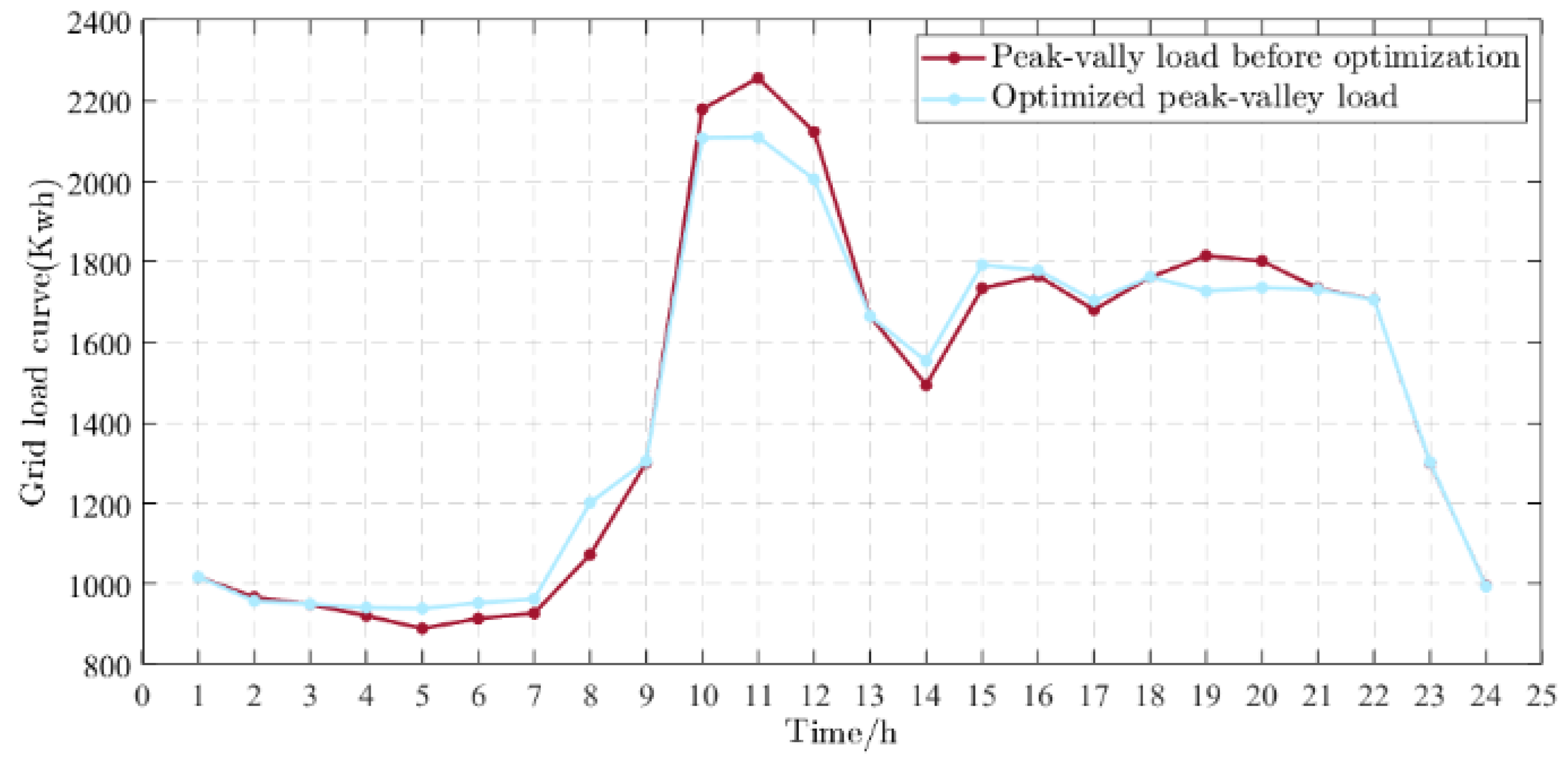
- The three objective functions proposed in this paper can effectively reduce the operating costs of the integrated energy station and the pollutant emissions from the station and, at the same time, reduce the peak-to-valley load difference of the regional power system, so as to achieve a balance of interests between the integrated energy system and the power grid.
- (3)
- A multi-objective optimization algorithm (NSNGO) based on the non-dominated sorting northern pale eagle high-latitude multi-objective optimization algorithm (NSNGO) is proposed, which is shown to be excellent in generating high-quality optimal solutions through a comparative analysis, and an evaluation index convergence metric (CM) for evaluating the extent of the global search/local search is also proposed, which is capable of reflecting whether or not the algorithm has sufficiently explored the search space.
- (4)
- An energy management strategy for storage prioritization is proposed to determine the optimal allocation of storage capacity by exploring the impacts of three energy sources under different storage prioritization levels, thus helping to effectively manage energy resources and ensure sustainable operation.
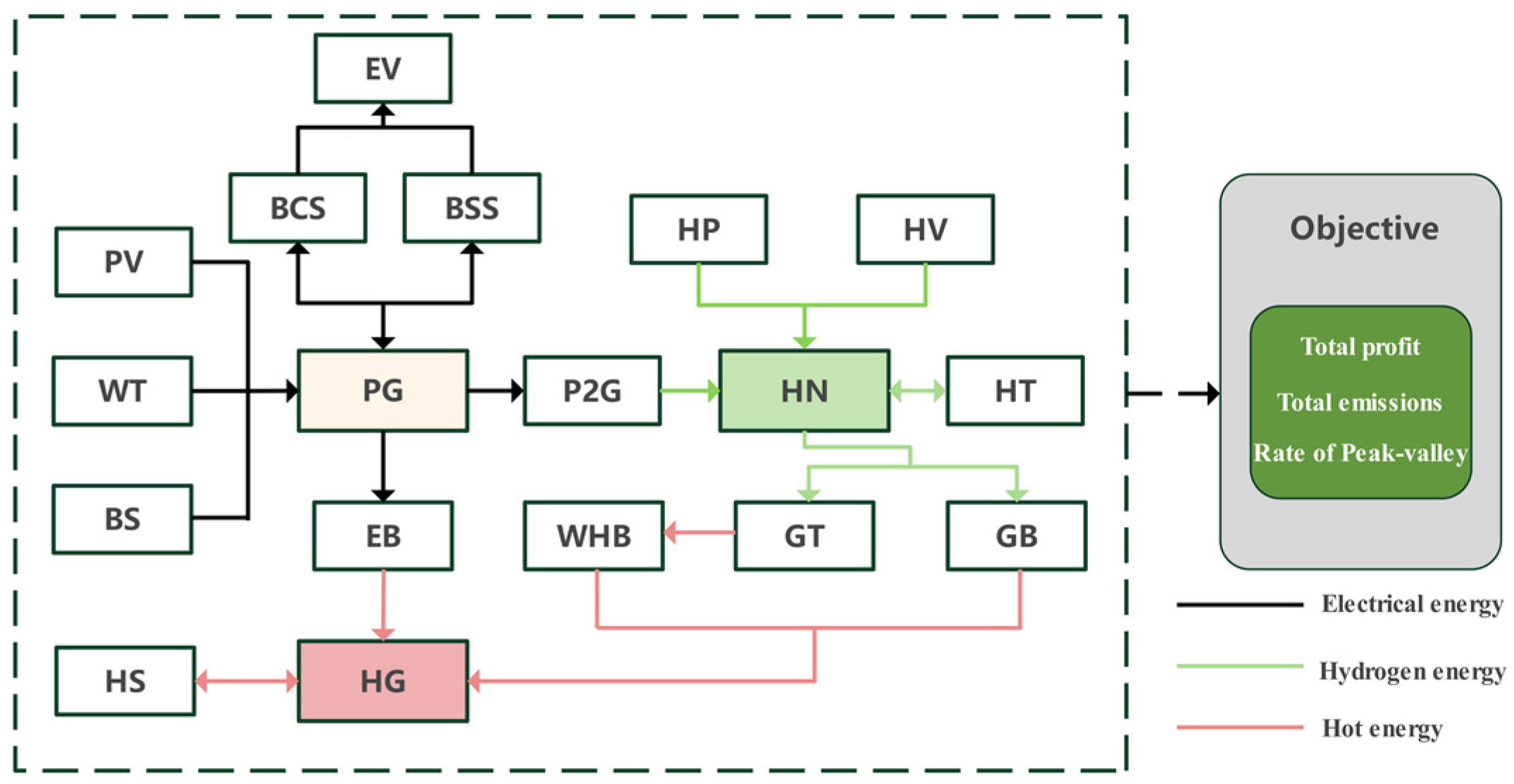
2. Multi-Energy-Coupled Integrated Energy System Structure and Modeling
- (1)
- Power load supply:
- (2)
- Heat load supply:
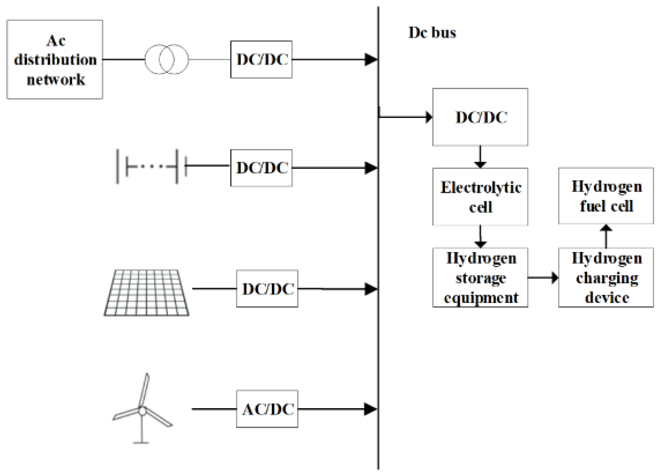
- (3)
- Hydrogen production and storage:
- (4)
- Network Integration:
2.1. Wind Turbine Model
2.2. Photovoltaic Model
2.3. Hydrogen Production System Model
2.3.1. Electrolyzer Model
2.3.2. Compressor Model
2.3.3. Hydrogen Storage Tank Model
2.4. Heat Production Model
2.4.1. Gas Turbine Model
2.4.2. Gas Boiler Model
2.4.3. Waste Heat Boiler Model
2.5. Battery Energy Storage System Model
2.5.1. Battery Charging Station
2.5.2. Battery-Switching Station
2.6. Objective Function
2.6.1. Total Profit
2.6.2. Total Emissions
2.6.3. Rate of Peak–Valley
2.7. Constraints
2.7.1. Power Constraint
2.7.2. Electricity and Gas Purchase Constraints
2.7.3. Capacity Constraint
2.8. Energy Storage Prioritization Strategy
3. Solution Method
3.1. Northern Goshawk Optimization
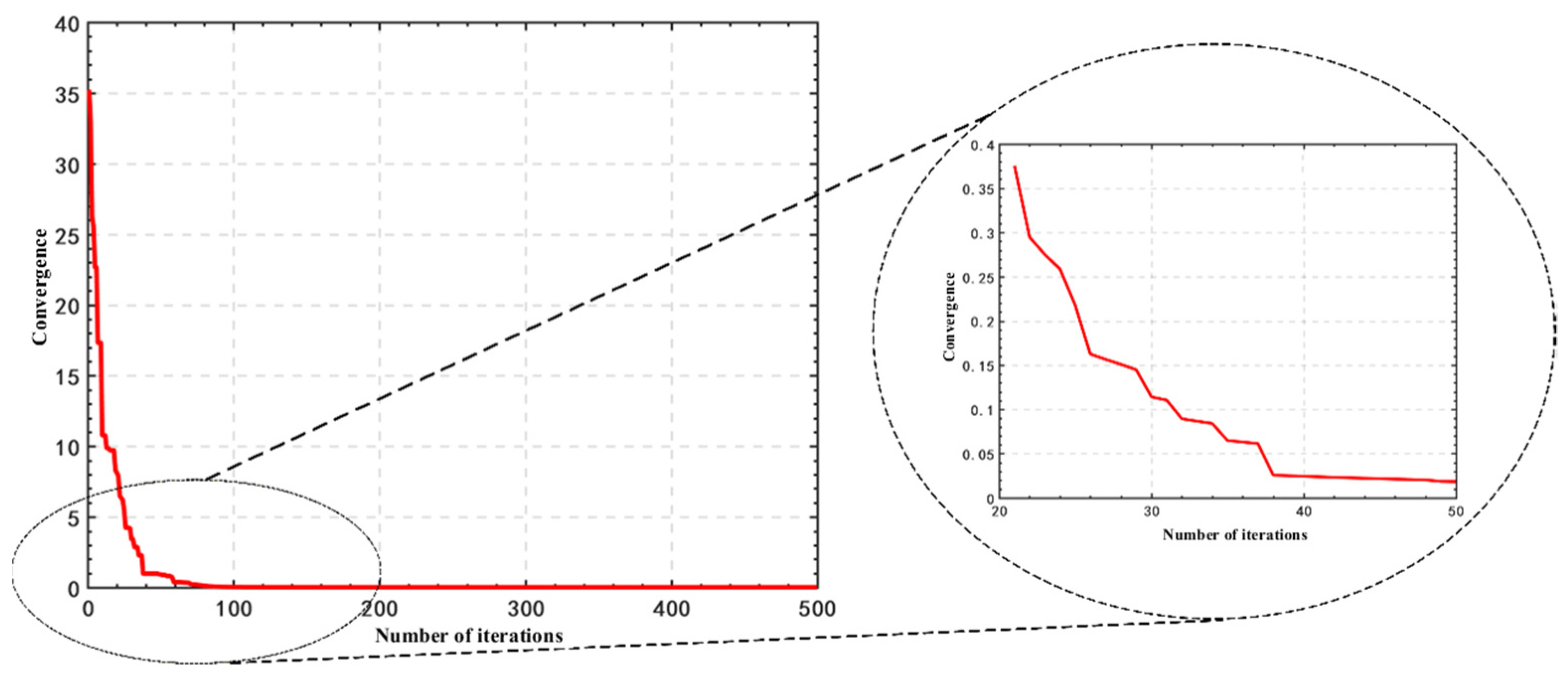
3.2. Convergence Metric
- Calculate the Euclidean distance from the individual to all reference points, :where is the dimension of the problem.
- For each individual , calculate its average distance to all reference points:
- Calculate the average distance across the population:
3.3. Parameter Sensitivity Analysis
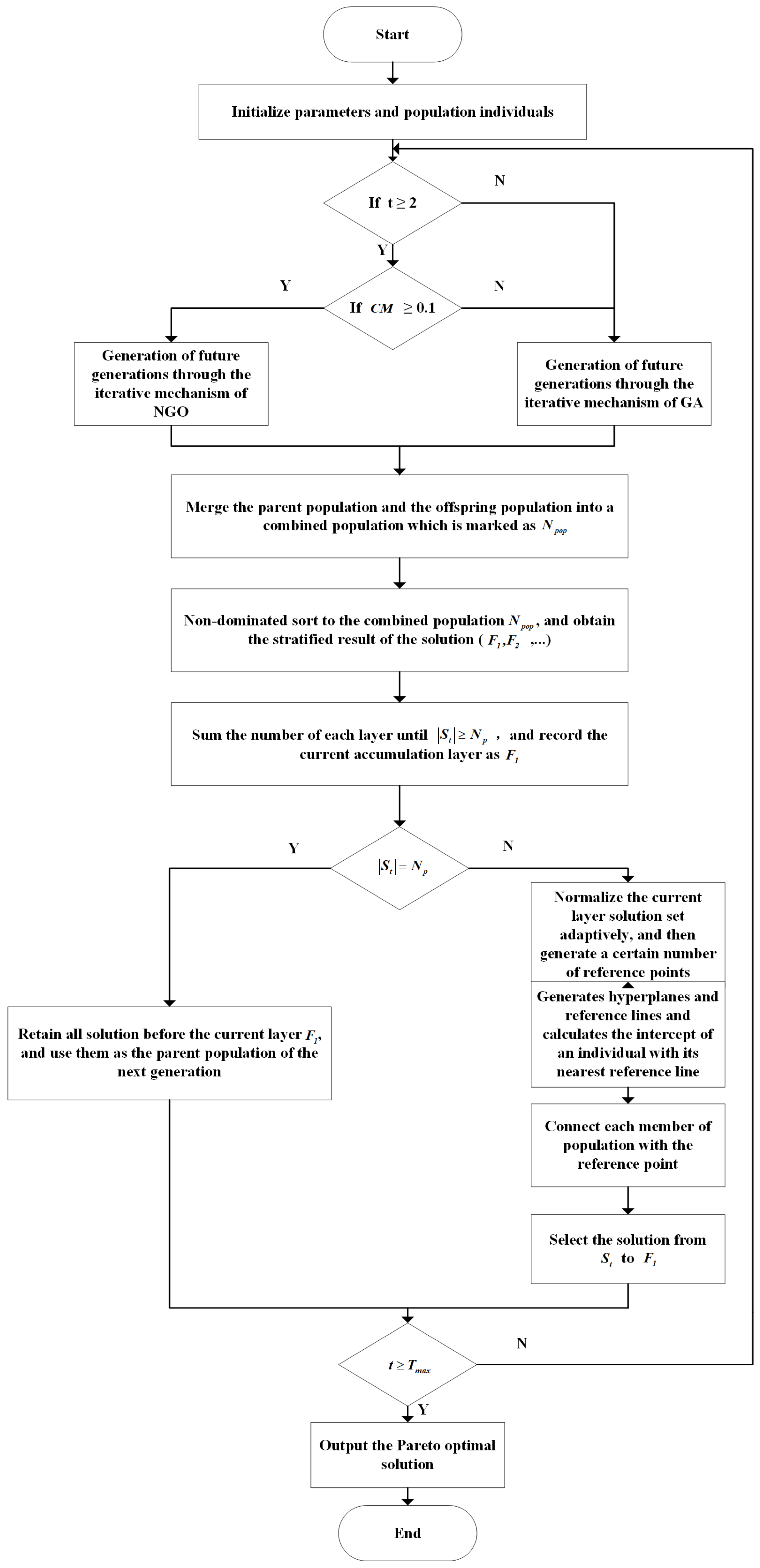
3.4. Non-Dominated Sorting Genetic Northern Goshawk Optimization
| Algorithm 1 Implementation process of the NSNGO algorithm |
| Input: Define the initial number of populations, ; the maximum number of iterations, ; the parent population, ; and the iterated offspring population, 1: for then 2: elseif flag = 0 3: % Combining Survival Strategies in DOA with NGO Algorithms 4: for : do 5: % C is a balancing parameter between exploration and exploitation 6: if k > 0.6 && rand1 < 0.5 do Then, update all individuals in the population 7: 8: elseif k > 0.6 && rand1 > 0.5 9: 10: elseif k < 0.6 && rand1 < 0.5 11: % is a uniformly generated random number in the interval [−1, 1], is the ith randomly selected individual, is a randomly generated binary number 12: elseif k < 0.6 && rand1 > 0.5 % is the best individual found in the previous iteration, the, was the th randomly selected individua. 13: end if 14: % Calculating the fitness of a population 15: Find the most adapted individual in the population , and record the coordinates of the individual with the best individual weight. 16: end for 17: elseif flag = 1 18: % GA 19: % Crossover + Mutation 20: end 21: After is performed, , 22: , 23: 24: Repeat 25: 26: Until 27: Last front to be included: 28: if then 29: 30: break 31: else 32: 33: Point to be chosen from , 34: Normalize the objective function and create a reference set , 35: and associated elements of reference points, 36: Select individuals from at a time to form 37: end if 38: end for |
| Determination conditions for localized search strategies |
| Input: Parent stock, ; iterated population of offspring, ; current number of iterations; current indicator value, Output: Local search operator flag 1: if t ≥ 2 then 2: Calculate the for the current iteration number t 3: if ≤ 0.1 then 4: flag = 1 5: else 6: flag = 0 7: end if 8: end if |
3.5. Comparison of Experimental Results
4. Experiments and Analysis of Results
4.1. Introduction to the Algorithm
4.2. Model Comparison Experiment
- Case (1)
- Case (2)
4.3. Typical Solution Analysis
- (1)
- Establish the virtual matrix:
- (2)
- Establishment of relative deviation fuzzy matrix:
- (3)
- Coefficient of variation method to determine the weight vector:
- (4)
- Weighting the deviations of the programs:
4.4. Analysis of the Results of the Optimized Scheduling Scheme
5. Conclusions
- (1)
- Technical maturity: Despite significant advancements in energy storage technologies in recent years, some technologies (such as certain novel battery technologies) may still be in the research and development stage or limited to small-scale applications, and have not yet reached the maturity level required for large-scale commercialization. Immature technologies may lead to performance instability, high maintenance costs, and safety issues, all of which pose potential obstacles during implementation.
- (2)
- Economic feasibility: The cost of energy storage technologies remains one of the primary limiting factors for their widespread adoption. Although costs are gradually decreasing with technological advancements and scale production, in some regions or application scenarios, the return on investment may still be insufficient to attract sufficient private capital. Furthermore, the economic benefits of energy storage technologies are influenced by various factors, such as energy prices, policy subsidies, and tax incentives.
- (3)
- Technical and system integration challenges: The application of energy storage technologies in integrated energy systems also faces technical and system integration challenges. Differences in performance among various energy storage technologies, compatibility with other energy systems, and technical difficulties during system integration can all affect the effectiveness of technology implementation.
Supplementary Materials
Author Contributions
Funding
Data Availability Statement
Acknowledgments
Conflicts of Interest
References
- Denholm, P.; Arent, D.J.; Baldwin, S.F.; Bilello, D.E.; Brinkman, G.L.; Cochran, J.M.; Cole, W.J.; Frew, B.; Gevorgian, V.; Heeter, J.; et al. The challenges of achieving a 100% renewable electricity system in the United States. Joule 2021, 5, 1331–1352. [Google Scholar] [CrossRef]
- Li, R.; Satchwell, A.J.; Finn, D.; Christensen, T.H.; Kummert, M.; Le Dréau, J.; Lopes, R.A.; Madsen, H.; Salom, J.; Henze, G.; et al. Ten questions concerning energy flexibility in buildings. Build. Environ. 2022, 223, 109461. [Google Scholar] [CrossRef]
- Zhao, D.; Xia, X.; Tao, R. Optimal configuration of electric-gas-thermal multi-energy storage system for regional integrated energy system. Energies 2019, 12, 2586. [Google Scholar] [CrossRef]
- Baniasadi, A.; Habibi, D.; Al-Saedi, W.; Masoum, M.A.S.; Das, C.K.; Mousavi, N. Optimal sizing design and operation of electrical and thermal energy storage systems in smart buildings. J. Energy Storage 2020, 28, 101186. [Google Scholar] [CrossRef]
- Zhu, Q.; Li, Q.; Zhang, B.; Wang, L.; Li, G.; Wang, R. Capacity optimization for electrical and thermal energy storage in multi-energy building energy system. Energy Procedia 2019, 158, 6425–6430. [Google Scholar] [CrossRef]
- Yan, Z.; Zhang, Y.; Liang, R.; Jin, W. An allocative method of hybrid electrical and thermal energy storage capacity for load shifting based on seasonal difference in district energy planning. Energy 2020, 207, 118139. [Google Scholar] [CrossRef]
- Guo, Y.; Wu, L.; Wang, C.; Guo, C.; Wu, D.; Zhang, Y. Optimal Configuration of Multi energy Storage for Load Aggregators Considering User Behavior 2020. In Proceedings of the IEEE/IAS Industrial and Commercial Power System Asia (I&CPS Asia), Weihai, China, 13–16 July 2020; pp. 1093–1101. [Google Scholar] [CrossRef]
- Bartolini, A.; Carducci, F.; Muñoz, C.B.; Comodi, G. Energy storage and multi energy systems in local energy communities with high renewable energy penetration. Renew. Energy 2020, 159, 595–609. [Google Scholar] [CrossRef]
- Luo, F.; Shao, J.; Jiao, Z.; Zhang, T. Research on optimal allocation strategy of multiple energy storage in regional integrated energy system based on operation benefit increment. Int. J. Electr. Power Energy Syst. 2021, 125, 106376. [Google Scholar] [CrossRef]
- Liu, Z.; Guo, J.; Wu, D.; Fan, G.; Zhang, S.; Yang, X.; Ge, H. Two-phase collaborative optimization and operation strategy for a new distributed energy system that combines multi-energy storage for a nearly zero energy community. Energy Convers. Manag. 2021, 230, 113800. [Google Scholar] [CrossRef]
- Liu, J.; Cao, S.; Chen, X.; Yang, H.; Peng, J. Energy planning of renewable applications in high-rise residential buildings integrating battery and hydrogen vehicle storage. Appl. Energy 2021, 28, 116038. [Google Scholar] [CrossRef]
- Dik, A.; Kutlu, C.; Omer, S.; Boukhanouf, R.; Su, Y.; Riffat, S. An approach for energy management of renewable energy sources using electric vehicles and heat pumps in an integrated electricity grid system. Energy Build. 2023, 294, 113261. [Google Scholar] [CrossRef]
- Agberegha, L.O.; Aigba, P.A.; Nwigbo, S.C.; Onoroh, F.; Samuel, O.D.; Bako, T.; Der, O.; Ercetin, A.; Sener, R. Investigation of a Hybridized Cascade Trigeneration Cycle Combined with a District Heating and Air Conditioning System Using Vapour Absorption Refrigeration Cooling: Energy and Exergy Assessments. Energies 2024, 17, 1295. [Google Scholar] [CrossRef]
- Amir Ahmarinejad, A Multi-objective Optimization Framework for Dynamic Planning of Energy Hub Considering Integrated Demand Response Program. Sustain. Cities Soc. 2021, 74, 103136. [CrossRef]
- Li, J.H.; Chen, G.Y.; Li, M.; Chen, H. An Adaptative Reference Vector Based Evolutionary Algorithm for Many-Objective Optimization. IEEE Access 2019, 7, 80506–80518. [Google Scholar] [CrossRef]
- Yang, F.; Wang, S.W.; Zhang, J.X.; Gao, N.; Qu, J.F. An Angle-Based Bi-Objective Evolutionary Algorithm for Many-Objective Optimization. IEEE Access 2020, 8, 194015–194026. [Google Scholar] [CrossRef]
- Jiang, S.Y.; He, X.Y.; Zhou, Y.R. Many-objective evolutionary algorithm based on adaptive weighted decomposition. Appl. Soft Comput. 2019, 84, 105731. [Google Scholar] [CrossRef]
- Jiang, S.Y.; Yang, S.X. A Strength Pareto Evolutionary Algorithm Based on Reference Direction for Multiobjective and Many-Objective Optimization. IEEE Trans. Evol. Comput. 2017, 21, 329–346. [Google Scholar] [CrossRef]
- Chen, S.Y.; Wang, X.W.; Gao, J.; Du, W.; Gu, X.S. An adaptive switching-based evolutionary algorithm for many-objective optimization. Knowl.-Based Syst. 2022, 248, 108915. [Google Scholar] [CrossRef]
- Sun, Y.H.; Xiao, K.L.; Wang, S.Q.; Lv, Q.Y. An evolutionary many-objective algorithm based on decomposition and hierarchical clustering selection. Appl. Intell. 2022, 52, 8464–8509. [Google Scholar] [CrossRef]
- Zhang, Z.X.; Wen, J.; Zhang, J.J.; Cai, X.J.; Xie, L.P. A Many Objective-Based Feature Selection Model for Anomaly Detection in Cloud Environment. IEEE Access 2020, 8, 60218–60231. [Google Scholar] [CrossRef]
- Jain, H.; Deb, K. An Evolutionary Many-Objective Optimization Algorithm Using Reference-Point Based Nondominated Sorting Approach, Part II: Handling Constraints and Extending to an Adaptive Approach. IEEE Trans. Evol. Comput. 2014, 18, 602–622. [Google Scholar] [CrossRef]
- Xu, X.; Hu, W.H.; Cao, D.; Huang, Q.; Chen, C.; Chen, Z. Optimized sizing of a standalone PV-wind-hydropower station with pumped-storage installation hybrid energy system. Renew. Energy 2020, 147, 1418–1431. [Google Scholar] [CrossRef]
- Gökmen, N.; Hu, W.H.; Hou, P.; Chen, Z.; Sera, D.; Spataru, S. Investigation of wind speed cooling effect on PV panels in windy locations. Renew. Energy 2016, 90, 283–290. [Google Scholar] [CrossRef]
- Micena, R.P.; Llerena-Pizarro, O.R.; de Souza, T.M.; Silveira, J.L. Solar-powered Hydrogen Refueling Stations: A techno-economic analysis. Int. J. Hydrogen Energy 2020, 45, 2308–2318. [Google Scholar] [CrossRef]
- Li, C.-H.; Zhu, X.-J.; Cao, G.-Y.; Sui, S.; Hu, M.-R. Dynamic modeling and sizing optimization of stand-alone photovoltaic power systems using hybrid energy storage technology. Renew. Energy 2009, 34, 815–826. [Google Scholar] [CrossRef]
- Farzin, H.; Fotuhi-Firuzabad, M.; Moeini-Aghtaie, M. A Practical Scheme to Involve Degradation Cost of Lithium-Ion Batteries in Vehicle-to-Grid Applications. IEEE Trans. Sustain. Energy 2016, 7, 1730–1738. [Google Scholar] [CrossRef]
- Bibak, B.; Tekiner-Mogulkoc, H. The parametric analysis of the electric vehicles and vehicle to grid system’s role in flattening the power demand. Sustain. Energy Grids 2022, 30, 100605. [Google Scholar] [CrossRef]
- Liang, H.J.; Liu, Y.G.; Li, F.Z.; Shen, Y.J. Dynamic Economic/Emission Dispatch Including PEVs for Peak Shaving and Valley Filling. IEEE Trans. Ind. Electron. 2019, 66, 2880–2890. [Google Scholar] [CrossRef]
- Wang, Z.P.; Wang, S. Grid Power Peak Shaving and Valley Filling Using Vehicle-to-Grid Systems. IEEE Trans. Power Deliv. 2013, 28, 1822–1829. [Google Scholar] [CrossRef]
- Guo, L.; Liu, W.J.; Jiao, B.Q.; Hong, B.W.; Wang, C.S. Multi-objective stochastic optimal planning method for stand-alone microgrid system. IET Gener. Transm. Dis. 2014, 8, 1263–1273. [Google Scholar] [CrossRef]
- Dehghani, M.; Hubálovsky, S.; Trojovsky, P. Northern Goshawk Optimization: A New Swarm-Based Algorithm for Solving Optimization Problems. IEEE Access 2021, 9, 162059–162080. [Google Scholar] [CrossRef]
- Sun, B.J. A multi-objective optimization model for fast electric vehicle charging stations with wind, PV power and energy storage. J. Clean. Prod. 2021, 288, 125564. [Google Scholar] [CrossRef]
- Samuel, O.D.; Aigba, P.A.; Tran, T.K.; Fayaz, H.; Pastore, C.; Der, O.; Erçetin, A.; Enweremadu, C.C.; Mustafa, A. Comparison of the Techno-Economic and Environmental Assessment of Hydrodynamic Cavitation and Mechanical Stirring Reactors for the Production of Sustainable Hevea brasiliensis Ethyl Ester. Sustainability 2023, 15, 16287. [Google Scholar] [CrossRef]


| Norm | Number of Iterations | ||||||
|---|---|---|---|---|---|---|---|
| CM | 20 | 21 | 22 | 23 | 24 | 25 | 26 |
| 8.11 | 7.89 | 6.49 | 6.33 | 6.21 | 5.45 | 4.23 | |
| CM | 27 | 28 | 29 | 30 | 31 | 32 | 33 |
| 4.22 | 4.23 | 4.20 | 3.43 | 3.43 | 2.86 | 2.86 | |
| CM | 34 | 35 | 36 | 37 | 38 | 39 | 40 |
| 2.86 | 2.27 | 2.27 | 2.27 | 0.98 | 0.97 | 0.97 | |
| CM | 41 | 42 | 43 | 44 | 45 | 46 | 47 |
| 0.98 | 0.98 | 0.98 | 0.98 | 0.98 | 0.98 | 0.98 | |
| CM | 48 | 49 | 50 | ||||
| 0.98 | 0.98 | 0.93 | |||||
| Function | Dimension | MAX Gen | 0.01 | 0.05 | 0.1 | 0.5 | 1 |
|---|---|---|---|---|---|---|---|
| DTLZ1 | 3 | 400 | 2.15 × 10⁻⁴ | 1.92 × 10⁻⁴ | 2.09 × 10⁻⁴ | 4.90 × 10⁻⁴ | 3.18 × 10⁻⁴ |
| 1.72 × 10⁻⁴ | 1.68 × 10⁻⁴ | 1.64 × 10⁻⁴ | 1.69 × 10⁻⁴ | 1.75 × 10⁻⁴ | |||
| 1.83 × 10⁻⁴ | 1.80 × 10⁻⁴ | 1.80 × 10⁻⁴ | 2.20 × 10⁻⁴ | 2.00 × 10⁻⁴ | |||
| 5 | 600 | 1.09 × 10⁻³ | 1.25 × 10⁻³ | 4.22 × 10⁻⁴ | 3.89 × 10⁻⁴ | 5.99 × 10⁻⁴ | |
| 3.24 × 10⁻⁴ | 2.72 × 10⁻⁴ | 2.57 × 10⁻⁴ | 2.68 × 10⁻⁴ | 2.79 × 10⁻⁴ | |||
| 4.46 × 10⁻⁴ | 4.80 × 10⁻⁴ | 3.32 × 10⁻⁴ | 3.44 × 10⁻⁴ | 3.82 × 10⁻⁴ | |||
| 8 | 750 | 1.05 × 10⁻¹ | 7.50 × 10⁻² | 6.74 × 10⁻² | 9.89 × 10⁻² | 8.44 × 10⁻² | |
| 1.87 × 10⁻³ | 1.99 × 10⁻³ | 1.86 × 10⁻³ | 2.37 × 10⁻³ | 1.96 × 10⁻³ | |||
| 1.28 × 10⁻² | 1.45 × 10⁻² | 8.98 × 10⁻³ | 2.07 × 10⁻² | 1.42 × 10⁻² | |||
| 10 | 1000 | 2.12 × 10⁻¹ | 1.00 × 10⁻¹ | 8.80 × 10⁻² | 2.90 × 10⁻¹ | 8.97 × 10⁻² | |
| 3.56 × 10⁻³ | 3.32 × 10⁻³ | 3.01 × 10⁻³ | 3.88 × 10⁻³ | 3.52 × 10⁻³ | |||
| 4.04 × 10⁻² | 2.15 × 10⁻² | 3.19 × 10⁻² | 4.73 × 10⁻² | 1.77 × 10⁻² | |||
| 15 | 1500 | 2.09 × 10⁻¹ | 2.30 × 10⁻¹ | 2.06 × 10⁻¹ | 2.21 × 10⁻¹ | 2.34 × 10⁻¹ | |
| 8.12 × 10⁻³ | 3.73 × 10⁻³ | 3.38 × 10⁻³ | 6.31 × 10⁻³ | 7.99 × 10⁻³ | |||
| 1.22 × 10⁻¹ | 1.36 × 10⁻¹ | 1.20 × 10⁻¹ | 1.00 × 10⁻¹ | 9.70 × 10⁻² | |||
| DTLZ2 | 3 | 250 | 5.78 × 10⁻⁴ | 5.93 × 10⁻⁴ | 5.34 × 10⁻⁴ | 6.25 × 10⁻⁴ | 5.75 × 10⁻⁴ |
| 4.53 × 10⁻⁴ | 4.74 × 10⁻⁴ | 4.04 × 10⁻⁴ | 4.27 × 10⁻⁴ | 4.37 × 10⁻⁴ | |||
| 4.90 × 10⁻⁴ | 5.19 × 10⁻⁴ | 4.82 × 10⁻⁴ | 5.01 × 10⁻⁴ | 5.02 × 10⁻⁴ | |||
| 5 | 350 | 1.29 × 10⁻³ | 1.21 × 10⁻³ | 1.13 × 10⁻³ | 1.23 × 10⁻³ | 1.09 × 10⁻³ | |
| 8.71 × 10⁻⁴ | 9.31 × 10⁻⁴ | 7.92 × 10⁻⁴ | 9.39 × 10⁻⁴ | 9.34 × 10⁻⁴ | |||
| 1.06 × 10⁻³ | 1.08 × 10⁻³ | 9.51 × 10⁻⁴ | 1.10 × 10⁻³ | 1.01 × 10⁻³ | |||
| 8 | 500 | 2.73 × 10⁻² | 5.23 × 10⁻³ | 4.83 × 10⁻³ | 5.38 × 10⁻³ | 5.45 × 10⁻³ | |
| 4.61 × 10⁻³ | 4.37 × 10⁻³ | 4.02 × 10⁻³ | 4.52 × 10⁻³ | 4.16 × 10⁻³ | |||
| 7.32 × 10⁻³ | 4.81 × 10⁻³ | 4.50 × 10⁻³ | 4.87 × 10⁻³ | 4.57 × 10⁻³ | |||
| 10 | 750 | 3.49 × 10⁻¹ | 1.08 × 10⁻² | 1.03 × 10⁻² | 3.79 × 10⁻¹ | 4.05 × 10⁻¹ | |
| 7.78 × 10⁻³ | 7.43 × 10⁻³ | 7.29 × 10⁻³ | 7.99 × 10⁻³ | 7.64 × 10⁻³ | |||
| 4.28 × 10⁻² | 8.56 × 10⁻³ | 8.33 × 10⁻³ | 8.25 × 10⁻² | 1.11 × 10⁻¹ | |||
| 15 | 1000 | 4.84 × 10⁻¹ | 3.98 × 10⁻¹ | 2.33 × 10⁻¹ | 2.38 × 10⁻¹ | 3.44 × 10⁻¹ | |
| 9.80 × 10⁻³ | 1.03 × 10⁻² | 1.00 × 10⁻² | 9.33 × 10⁻³ | 9.27 × 10⁻³ | |||
| 1.67 × 10⁻¹ | 1.71 × 10⁻¹ | 3.60 × 10⁻² | 5.10 × 10⁻² | 1.34 × 10⁻¹ | |||
| DTLZ3 | 3 | 1000 | 1.52 × 10⁻³ | 1.27 × 10⁻³ | 2.47 × 10⁻⁴ | 2.49 × 10⁻⁴ | 3.12 × 10⁻⁴ |
| 2.00 × 10⁻⁴ | 2.01 × 10⁻⁴ | 1.18 × 10⁻⁴ | 1.84 × 10⁻⁴ | 1.80 × 10⁻⁴ | |||
| 4.24 × 10⁻⁴ | 3.51 × 10⁻⁴ | 1.98 × 10⁻⁴ | 2.01 × 10⁻⁴ | 2.07 × 10⁻⁴ | |||
| 5 | 1000 | 1.84 × 10⁻³ | 1.56 × 10⁻³ | 6.94 × 10⁻⁴ | 6.66 × 10⁻⁴ | 6.83 × 10⁻⁴ | |
| 6.79 × 10⁻⁴ | 5.97 × 10⁻⁴ | 4.03 × 10⁻⁴ | 5.77 × 10⁻⁴ | 5.92 × 10⁻⁴ | |||
| 8.69 × 10⁻⁴ | 7.75 × 10⁻⁴ | 6.03 × 10⁻⁴ | 6.09 × 10⁻⁴ | 6.31 × 10⁻⁴ | |||
| 8 | 1000 | 8.71 × 10⁻³ | 6.33 × 10⁻³ | 5.59 × 10⁻³ | 6.20 × 10⁻³ | 4.25 × 10⁻¹ | |
| 5.06 × 10⁻³ | 4.44 × 10⁻³ | 4.06 × 10⁻³ | 4.82 × 10⁻³ | 4.45 × 10⁻³ | |||
| 6.40 × 10⁻³ | 5.09 × 10⁻³ | 4.84 × 10⁻³ | 5.39 × 10⁻³ | 4.70 × 10⁻² | |||
| 10 | 1500 | 5.97 × 10⁻¹ | 8.05 × 10⁻¹ | 5.43 × 10⁻¹ | 5.66 × 10⁻¹ | 5.48 × 10⁻¹ | |
| 7.01 × 10⁻³ | 7.43 × 10⁻³ | 6.61 × 10⁻³ | 7.18 × 10⁻³ | 7.07 × 10⁻³ | |||
| 2.73 × 10⁻¹ | 3.98 × 10⁻¹ | 2.54 × 10⁻¹ | 2.71 × 10⁻¹ | 3.63 × 10⁻¹ | |||
| 15 | 2000 | 5.34 × 10⁻¹ | 5.23 × 10⁻¹ | 5.44 × 10⁻¹ | 5.56 × 10⁻¹ | 5.82 × 10⁻¹ | |
| 4.68 × 10⁻¹ | 4.31 × 10⁻¹ | 9.66 × 10⁻² | 1.10 × 10⁻¹ | 4.95 × 10⁻¹ | |||
| 4.99 × 10⁻¹ | 4.91 × 10⁻¹ | 4.65 × 10⁻¹ | 4.83 × 10⁻¹ | 5.26 × 10⁻¹ | |||
| DTLZ4 | 3 | 600 | 1.62 × 10⁻³ | 1.90 × 10⁻³ | 1.36 × 10⁻³ | 1.57 × 10⁻³ | 9.48 × 10⁻¹ |
| 3.11 × 10⁻⁴ | 2.63 × 10⁻⁴ | 2.51 × 10⁻⁴ | 2.85 × 10⁻⁴ | 5.37 × 10⁻¹ | |||
| 8.22 × 10⁻⁴ | 7.08 × 10⁻⁴ | 7.21 × 10⁻⁴ | 8.08 × 10⁻⁴ | 7.83 × 10⁻¹ | |||
| 5 | 1000 | 1.45 × 10⁻³ | 1.60 × 10⁻³ | 1.24 × 10⁻³ | 1.37 × 10⁻³ | 4.04 × 10⁻¹ | |
| 9.17 × 10⁻⁴ | 8.27 × 10⁻⁴ | 8.03 × 10⁻⁴ | 1.02 × 10⁻³ | 9.41 × 10⁻⁴ | |||
| 1.16 × 10⁻³ | 1.07 × 10⁻³ | 1.06 × 10⁻³ | 1.22 × 10⁻³ | 7.77 × 10⁻² | |||
| 8 | 1250 | 4.74 × 10⁻³ | 4.41 × 10⁻³ | 4.24 × 10⁻³ | 4.86 × 10⁻³ | 4.36 × 10⁻³ | |
| 3.64 × 10⁻³ | 3.50 × 10⁻³ | 2.72 × 10⁻³ | 3.45 × 10⁻³ | 3.46 × 10⁻³ | |||
| 4.15 × 10⁻³ | 3.98 × 10⁻³ | 3.84 × 10⁻³ | 4.19 × 10⁻³ | 3.92 × 10⁻³ | |||
| 10 | 2000 | 5.51 × 10⁻³ | 5.34 × 10⁻³ | 5.93 × 10⁻³ | 5.19 × 10⁻³ | 5.49 × 10⁻³ | |
| 4.45 × 10⁻³ | 4.05 × 10⁻³ | 4.01 × 10⁻³ | 4.29 × 10⁻³ | 4.32 × 10⁻³ | |||
| 5.09 × 10⁻³ | 4.68 × 10⁻³ | 4.61 × 10⁻³ | 4.65 × 10⁻³ | 4.89 × 10⁻³ | |||
| 15 | 3000 | 6.83 × 10⁻³ | 6.70 × 10⁻³ | 6.54 × 10⁻³ | 6.92 × 10⁻³ | 7.81 × 10⁻³ | |
| 4.97 × 10⁻³ | 5.31 × 10⁻³ | 5.21 × 10⁻³ | 5.35 × 10⁻³ | 5.02 × 10⁻³ | |||
| 5.99 × 10⁻³ | 5.85 × 10⁻³ | 5.80 × 10⁻³ | 6.16 × 10⁻³ | 6.00 × 10⁻³ |
| Functions | m | Maxgen | NSNGO | NSGA-III | θ-DEA | MOEA/D-PBI |
|---|---|---|---|---|---|---|
| DTLZ1 | 3 | 400 | 1.74 × 10⁻⁴ | 4.88 × 10⁻⁴ | 5.66 × 10⁻⁴ | 4.10 × 10⁻⁴ |
| 1.85 × 10⁻⁴ | 1.31 × 10⁻³ | 1.31 × 10⁻³ | 1.50 × 10⁻³ | |||
| 2.01 × 10⁻⁴ | 4.88 × 10⁻³ | 9.45 × 10⁻³ | 4.74 × 10⁻³ | |||
| 5 | 600 | 1.71 × 10⁻⁵ | 5.12 × 10⁻⁴ | 4.43 × 10⁻⁴ | 3.18 × 10⁻⁴ | |
| 2.92 × 10⁻⁴ | 9.79 × 10⁻⁴ | 7.33 × 10⁻⁴ | 6.37 × 10⁻⁴ | |||
| 3.17 × 10⁻⁴ | 1.98 × 10⁻³ | 2.14 × 10⁻³ | 1.64 × 10⁻³ | |||
| 8 | 750 | 1.30 × 10⁻³ | 2.04 × 10⁻³ | 1.98 × 10⁻³ | 3.91 × 10⁻³ | |
| 1.60 × 10⁻³ | 3.89 × 10⁻³ | 2.70 × 10⁻³ | 6.11 × 10⁻³ | |||
| 2.00 × 10⁻³ | 8.72 × 10⁻³ | 4.62 × 10⁻³ | 8.54 × 10⁻³ | |||
| 10 | 1000 | 2.00 × 10⁻³ | 2.22 × 10⁻³ | 2.10 × 10⁻³ | 3.87 × 10⁻³ | |
| 4.05 × 10⁻³ | 3.46 × 10⁻³ | 2.45 × 10⁻³ | 5.07 × 10⁻³ | |||
| 6.50 × 10⁻³ | 6.87 × 10⁻³ | 3.94 × 10⁻³ | 6.03 × 10⁻³ | |||
| 15 | 1500 | 4.70 × 10⁻³ | 2.65 × 10⁻³ | 2.44 × 10⁻³ | 1.24 × 10⁻² | |
| 4.404 × 10⁻³ | 5.06 × 10⁻² | 8.15 × 10⁻³ | 1.53 × 10⁻² | |||
| 9.97 × 10⁻² | 1.12 × 10⁻² | 2.24 × 10⁻¹ | 1.69 × 10⁻² | |||
| DTLZ2 | 3 | 400 | 8.71 × 10⁻⁴ | 1.26 × 10⁻³ | 1.04 × 10⁻³ | 5.43 × 10⁻⁴ |
| 9.84 × 10⁻⁴ | 1.36 × 10⁻³ | 1.57 × 10⁻³ | 6.41 × 10⁻⁴ | |||
| 1.05 × 10⁻³ | 2.11 × 10⁻³ | 5.50 × 10⁻³ | 8.01 × 10⁻⁴ | |||
| 5 | 600 | 1.22 × 10⁻³ | 4.25 × 10⁻³ | 2.72 × 10⁻³ | 1.14 × 10⁻³ | |
| 1.44 × 10⁻³ | 4.98 × 10⁻³ | 3.25 × 10⁻³ | 2.26 × 10⁻³ | |||
| 1.73 × 10⁻³ | 5.86 × 10⁻³ | 5.33 × 10⁻³ | 2.65 × 10⁻³ | |||
| 8 | 750 | 4.98 × 10⁻³ | 1.37 × 10⁻² | 7.79 × 10⁻³ | 3.10 × 10⁻³ | |
| 6.00 × 10⁻³ | 1.57 × 10⁻² | 8.99 × 10⁻³ | 3.76 × 10⁻³ | |||
| 3.18 × 10⁻¹ | 1.81 × 10⁻² | 1.14 × 10⁻² | 5.20 × 10⁻³ | |||
| 10 | 1000 | 4.60 × 10⁻³ | 1.35 × 10⁻² | 7.56 × 10⁻³ | 2.47 × 10⁻³ | |
| 8.55 × 10⁻³ | 1.53 × 10⁻² | 8.81 × 10⁻³ | 2.78 × 10⁻³ | |||
| 5.65 × 10⁻¹ | 1.70 × 10⁻² | 1.02 × 10⁻² | 3.24 × 10⁻³ | |||
| 15 | 1500 | 1.67 × 10⁻² | 1.36 × 10⁻² | 8.82 × 10⁻³ | 5.25 × 10⁻³ | |
| 4.02 × 10⁻¹ | 1.73 × 10⁻² | 1.13 × 10⁻² | 6.01 × 10⁻³ | |||
| 4.80 × 10⁻¹ | 2.11 × 10⁻² | 1.48 × 10⁻² | 9.41 × 10⁻³ | |||
| DTLZ3 | 3 | 400 | 2.03 × 10⁻⁴ | 9.75 × 10⁻⁴ | 1.34 × 10⁻³ | 9.77 × 10⁻⁴ |
| 2.30 × 10⁻⁴ | 4.01 × 10⁻³ | 3.54 × 10⁻³ | 3.43 × 10⁻³ | |||
| 5.73 × 10⁻⁴ | 6.67 × 10⁻³ | 5.53 × 10⁻³ | 9.11 × 10⁻³ | |||
| 5 | 600 | 5.83 × 10⁻⁴ | 3.09 × 10⁻³ | 1.98 × 10⁻³ | 1.13 × 10⁻³ | |
| 6.65 × 10⁻⁴ | 5.96 × 10⁻³ | 4.27 × 10⁻³ | 2.21 × 10⁻³ | |||
| 7.87 × 10⁻³ | 1.20 × 10⁻² | 1.91 × 10⁻² | 6.15 × 10⁻³ | |||
| 8 | 750 | 2.79 × 10⁻³ | 1.24 × 10⁻² | 8.77 × 10⁻³ | 6.46 × 10⁻³ | |
| 3.11 × 10⁻³ | 2.38 × 10⁻² | 1.54 × 10⁻² | 1.95 × 10⁻² | |||
| 4.04 × 10⁻³ | 9.65 × 10⁻² | 3.83 × 10⁻² | 1.12 × 100 | |||
| 10 | 1000 | 3.50 × 10⁻³ | 8.85 × 10⁻³ | 5.97 × 10⁻³ | 2.79 × 10⁻³ | |
| 5.75 × 10⁻² | 1.19 × 10⁻² | 7.24 × 10⁻³ | 4.32 × 10⁻³ | |||
| 6.22 × 10⁻¹ | 2.08 × 10⁻² | 2.32 × 10⁻² | 1.01 × 100 | |||
| 15 | 1500 | 1.28 × 10⁻² | 1.40 × 10⁻² | 9.83 × 10⁻³ | 4.36 × 10⁻³ | |
| 5.56 × 10⁻¹ | 2.15 × 10⁻² | 1.92 × 10⁻² | 1.66 × 10⁻² | |||
| 6.38 × 10⁻¹ | 4.20 × 10⁻² | 6.21 × 10⁻¹ | 1.26 × 100 | |||
| DTLZ4 | 3 | 400 | 3.09 × 10⁻⁴ | 2.92 × 10⁻⁴ | 1.87 × 10⁻⁴ | 2.93 × 10⁻¹ |
| 5.70 × 10⁻⁴ | 5.97 × 10⁻⁴ | 2.51 × 10⁻⁴ | 4.28 × 10⁻¹ | |||
| 3.56 × 10⁻³ | 4.29 × 10⁻¹ | 5.32 × 10⁻¹ | 5.23 × 10⁻¹ | |||
| 5 | 600 | 7.81 × 10⁻⁴ | 9.85 × 10⁻⁴ | 2.62 × 10⁻⁴ | 1.08 × 10⁻¹ | |
| 1.05 × 10⁻³ | 1.26 × 10⁻³ | 3.79 × 10⁻⁴ | 5.79 × 10⁻¹ | |||
| 1.70 × 10⁻³ | 1.72 × 10⁻³ | 4.11 × 10⁻⁴ | 7.35 × 10⁻¹ | |||
| 8 | 750 | 2.38 × 10⁻³ | 5.08 × 10⁻³ | 2.78 × 10⁻³ | 5.30 × 10⁻¹ | |
| 3.05 × 10⁻³ | 7.05 × 10⁻³ | 3.10 × 10⁻³ | 8.82 × 10⁻¹ | |||
| 3.41 × 10⁻³ | 6.05 × 10⁻¹ | 3.57 × 10⁻³ | 9.72 × 10⁻¹ | |||
| 10 | 1000 | 2.62 × 10⁻³ | 5.69 × 10⁻³ | 2.75 × 10⁻³ | 3.97 × 10⁻¹ | |
| 3.50 × 10⁻³ | 6.34 × 10⁻³ | 3.34 × 10⁻³ | 9.20 × 10⁻¹ | |||
| 4.82 × 10⁻³ | 1.08 × 10⁻¹ | 3.91 × 10⁻³ | 1.08 × 100 | |||
| 15 | 1500 | 5.37 × 10⁻³ | 7.11 × 10⁻³ | 4.14 × 10⁻³ | 5.89 × 10⁻¹ | |
| 5.86 × 10⁻³ | 3.43 × 10⁻¹ | 5.90 × 10⁻³ | 1.13 × 100 | |||
| 6.88 × 10⁻³ | 1.073 × 10+ | 7.68 × 10⁻³ | 1.25 × 100 | |||
| DTLZ5 | 3 | 600 | 2.09 × 10⁻³ | 3.59 × 10⁻³ | 1.14 × 10⁻² | 2.38 × 10⁻³ |
| 2.60 × 10⁻³ | 4.37 × 10⁻³ | 1.30 × 10⁻² | 2.80 × 10⁻³ | |||
| 3.46 × 10⁻³ | 4.85 × 10⁻³ | 1.36 × 10⁻² | 3.76 × 10⁻³ | |||
| 5 | 1000 | 2.73 × 10⁻² | 4.35 × 10⁻² | 4.50 × 10⁻² | 2.05 × 10⁻² | |
| 4.78 × 10⁻² | 5.51 × 10⁻² | 8.75 × 10⁻² | 4.87 × 10⁻² | |||
| 6.12 × 10⁻² | 6.94 × 10⁻² | 1.28 × 10⁻¹ | 6.76 × 10⁻² | |||
| 8 | 1250 | 1.10 × 10⁻¹ | 1.44 × 10⁻¹ | 1.28 × 10⁻¹ | 3.87 × 10⁻² | |
| 1.83 × 10⁻¹ | 3.03 × 10⁻¹ | 1.47 × 10⁻¹ | 9.64 × 10⁻² | |||
| 2.30 × 10⁻¹ | 4.85 × 10⁻¹ | 1.97 × 10⁻¹ | 2.56 × 10⁻¹ | |||
| 10 | 2000 | 1.60 × 10⁻¹ | 2.15 × 10⁻¹ | 1.10 × 10⁻¹ | 4.78 × 10⁻² | |
| 2.47 × 10⁻¹ | 3.90 × 10⁻¹ | 1.47 × 10⁻¹ | 3.20 × 10⁻¹ | |||
| 3.85 × 10⁻¹ | 5.94 × 10⁻¹ | 1.97 × 10⁻¹ | 5.41 × 10⁻¹ | |||
| 15 | 3000 | 1.47 × 10⁻¹ | 2.19 × 10⁻¹ | 1.36 × 10⁻¹ | 7.49 × 10⁻² | |
| 2.69 × 10⁻¹ | 3.30 × 10⁻¹ | 2.87 × 10⁻¹ | 3.38 × 10⁻¹ | |||
| 3.71 × 10⁻¹ | 5.49 × 10⁻¹ | 4.22 × 10⁻¹ | 4.58 × 10⁻¹ | |||
| DTLZ6 | 3 | 600 | 3.95 × 10⁻³ | 4.38 × 10⁻³ | 1.37 × 10⁻² | 1.38 × 10⁻³ |
| 4.40 × 10⁻³ | 4.56 × 10⁻³ | 1.55 × 10⁻² | 1.42 × 10⁻³ | |||
| 5.02 × 10⁻³ | 4.79 × 10⁻³ | 1.69 × 10⁻² | 1.49 × 10⁻³ | |||
| 5 | 1000 | 2.24 × 10⁻² | 4.58 × 10⁻² | 1.35 × 10⁻¹ | 5.69 × 10⁻² | |
| 4.51 × 10⁻² | 5.77 × 10⁻² | 1.45 × 10⁻¹ | 9.85 × 10⁻² | |||
| 8.16 × 10⁻² | 7.96 × 10⁻² | 1.59 × 10⁻¹ | 1.77 × 10⁻¹ | |||
| 8 | 1250 | 1.23 × 10⁻¹ | 2.88 × 10⁻¹ | 1.99 × 10⁻¹ | 2.27 × 100 | |
| 2.41 × 10⁻¹ | 5.50 × 10⁻¹ | 2.66 × 10⁻¹ | 3.70 × 100 | |||
| 3.46 × 10⁻¹ | 7.42 × 10⁻¹ | 3.39 × 10⁻¹ | 4.39 × 100 | |||
| 10 | 2000 | 1.55 × 10⁻¹ | 3.29 × 10⁻¹ | 2.50 × 10⁻¹ | 3.30 × 100 | |
| 2.31 × 10⁻¹ | 5.31 × 10⁻¹ | 2.86 × 10⁻¹ | 4.93 × 100 | |||
| 3.04 × 10⁻¹ | 7.42 × 10⁻¹ | 3.33 × 10⁻¹ | 6.08 × 100 | |||
| 15 | 3000 | 1.83 × 10⁻¹ | 2.58 × 10⁻¹ | 2.39 × 10⁻¹ | 4.21 × 100 | |
| 2.80 × 10⁻¹ | 6.10 × 10⁻¹ | 3.04 × 10⁻¹ | 4.75 × 100 | |||
| 3.55 × 10⁻¹ | 7.42 × 10⁻¹ | 3.51 × 10⁻¹ | 5.30 × 100 | |||
| DTLZ7 | 3 | 600 | 4.76 × 10⁻² | 3.30 × 10⁻² | 5.94 × 10⁻² | 3.40 × 10⁻¹ |
| 1.85 × 10⁻¹ | 3.37 × 10⁻² | 7.06 × 10⁻² | 3.53 × 10⁻¹ | |||
| 7.31 × 10⁻¹ | 3.43 × 10⁻² | 9.13 × 10⁻² | 3.68 × 10⁻¹ | |||
| 5 | 1000 | 1.48 × 10⁻¹ | 2.05 × 10⁻¹ | 2.59 × 10⁻¹ | 2.43 × 10⁻¹ | |
| 1.92 × 10⁻¹ | 2.23 × 10⁻¹ | 2.65 × 10⁻¹ | 2.52 × 10⁻¹ | |||
| 2.46 × 10⁻¹ | 2.45 × 10⁻¹ | 2.74 × 10⁻¹ | 2.60 × 10⁻¹ | |||
| 8 | 1250 | 2.59 × 10⁻¹ | 5.64 × 10⁻¹ | 5.69 × 10⁻¹ | 1.04 × 100 | |
| 3.17 × 10⁻¹ | 6.05 × 10⁻¹ | 6.01 × 10⁻¹ | 1.09 × 100 | |||
| 4.82 × 10⁻¹ | 6.89 × 10⁻¹ | 6.46 × 10⁻¹ | 1.14 × 100 | |||
| 10 | 2000 | 3.28 × 10⁻¹ | 1.06 × 100 | 8.72 × 10⁻¹ | 1.59 × 100 | |
| 4.69 × 10⁻¹ | 1.22 × 100 | 9.86 × 10⁻¹ | 1.65 × 100 | |||
| 7.10 × 10⁻¹ | 1.43 × 100 | 1.09 × 100 | 1.69 × 100 | |||
| 15 | 3000 | 3.75 × 10⁻¹ | 1.88 × 100 | 3.20 × 100 | 2.20 × 100 | |
| 5.80 × 10⁻¹ | 1.96 × 100 | 3.75 × 100 | 2.31 × 100 | |||
| 8.76 × 10⁻¹ | 2.16 × 100 | 4.31 × 100 | 2.41 × 100 |
| Algorithm | Running Time | ||
|---|---|---|---|
| Best | Average | Worst | |
| NSGA-III | 11.7522 | 12.3023 | 12.6647 |
| ANSGA-III | 13.6241 | 14.4933 | 14.9921 |
| θ-DEA | 12.9632 | 13.6102 | 14.2424 |
| PREA | 21.8641 | 26.5847 | 30.2021 |
| NSNGO | 11.2712 | 11.6442 | 11.8733 |
| Installations | Life Span/a | Investment Cost/(yuan·kW−1) | Maintenance Cost/(yuan·kW−1) | Efficiency |
|---|---|---|---|---|
| WT | 25 | 10,000 | 0.01 | |
| PV | 25 | 12,000 | 0.01 | |
| ES | 20 | 800 | 0.15 | 0.9 |
| P2G | 15 | 3500 | 0.02 | 0.75 |
| HT | 10 | 300 | 0.02 | 0.9 |
| GT | 15 | 7800 | 0.01 | 0.7 |
| WHB | 15 | 200 | 0.05 | 0.4 |
| EB | 15 | 7500 | 0.01 | 0.9 |
| HS | 20 | 50 | 0.05 | 0.95 |
| m | |||||||||
|---|---|---|---|---|---|---|---|---|---|
| Value | 400 | 1000 | 60 kW·h | 20 | 15 | 5 | 50 Kg | 50 Kg | 60 Yuan/Kg |
| Load Type | Configuration Capacity |
|---|---|
| WT (kw·h) | 290 |
| PV (kw·h) | 290 |
| ES (kw·h) | 12 |
| P2Gr (kw·h) | 560 |
| HT (m)3 | 1800 |
| GB (kw·h) | 430 |
| GT (kw·h) | 13 |
| WHB (kw·h) | 106 |
| EB (kw·h) | 257 |
| HS (kw·h) | 364 |
| MET (kw·h) | 440 |
Disclaimer/Publisher’s Note: The statements, opinions and data contained in all publications are solely those of the individual author(s) and contributor(s) and not of MDPI and/or the editor(s). MDPI and/or the editor(s) disclaim responsibility for any injury to people or property resulting from any ideas, methods, instructions or products referred to in the content. |
© 2024 by the authors. Licensee MDPI, Basel, Switzerland. This article is an open access article distributed under the terms and conditions of the Creative Commons Attribution (CC BY) license (https://creativecommons.org/licenses/by/4.0/).
Share and Cite
Liao, X.; Lei, R.; Ouyang, S.; Huang, W. Capacity Optimization Allocation of Multi-Energy-Coupled Integrated Energy System Based on Energy Storage Priority Strategy. Energies 2024, 17, 5261. https://doi.org/10.3390/en17215261
Liao X, Lei R, Ouyang S, Huang W. Capacity Optimization Allocation of Multi-Energy-Coupled Integrated Energy System Based on Energy Storage Priority Strategy. Energies. 2024; 17(21):5261. https://doi.org/10.3390/en17215261
Chicago/Turabian StyleLiao, Xiang, Runjie Lei, Shuo Ouyang, and Wei Huang. 2024. "Capacity Optimization Allocation of Multi-Energy-Coupled Integrated Energy System Based on Energy Storage Priority Strategy" Energies 17, no. 21: 5261. https://doi.org/10.3390/en17215261
APA StyleLiao, X., Lei, R., Ouyang, S., & Huang, W. (2024). Capacity Optimization Allocation of Multi-Energy-Coupled Integrated Energy System Based on Energy Storage Priority Strategy. Energies, 17(21), 5261. https://doi.org/10.3390/en17215261