Article

Research on Power Device Fault Prediction of Rod Control Power Cabinet Based on Improved Dung Beetle Optimization–Temporal Convolutional Network Transfer Learning Model

1
School of Computer Science, University of South China, Hengyang 421200, China
2
Science and Technology on Reactor System Design Technology Laboratory, Nuclear Power Institute of China, Chengdu 610213, China
*
Author to whom correspondence should be addressed.
Energies 2024, 17(2), 447; https://doi.org/10.3390/en17020447
Submission received: 23 December 2023 / Revised: 8 January 2024 / Accepted: 11 January 2024 / Published: 16 January 2024
(This article belongs to the Section F: Electrical Engineering)

Abstract

:
In order to improve the reliability and maintainability of rod control power cabinets in nuclear power plants, this paper uses insulated gate bipolar transistors (IGBTs), the key power device of rod control power cabinets, as the object of research on cross-working-condition fault prediction. An improved transfer learning (TL) model based on a temporal convolutional network (TCN) is proposed to solve the problem of low fault prediction accuracy across operating conditions. First, the peak emitter voltage of an IGBT aging dataset is selected as the source domain failure characteristic, and the TCN model is trained after the removal of outliers and noise reduction. Then, the time–frequency features are extracted according to the characteristics of the target domain data, and the target domain representation data are obtained using kernel principal component analysis (KPCA) for dimensionality reduction. Finally, the TCN model trained on the source domain is transferred; the model is fine-tuned according to the target domain data, and the learning rate, the number of hidden layer nodes, and the number of training times in the network model are optimized using the dung beetle optimization (DBO) algorithm to obtain the optimal network, making it more suitable for target sample fault prediction. The prediction results of this TCN model, the long short-term memory (LSTM) model, the gated recurrent unit (GRU) model, and the recursive neural network (RNN) model are compared and analyzed by selecting prediction performance evaluation indexes. The results show that the TCN model has a better predictive effect. Comparing the prediction results of the TCN-based optimized transfer learning model with those of the directly trained TCN model, the mean square error, root mean square error, and mean absolute error are reduced by a factor of two to three, which provides an effective solution for fault prediction across operating conditions.

1. Introduction

The rod control system, which is a power control device for a control rod drive mechanism (CRDM), is a very important control system used in nuclear power plant reactors [1]. The rod control power cabinet is an important piece of equipment within a rod control system. Its function is to provide corresponding sequential currents to the three coils of the CRDM according to control commands so that the CRDM can be raised, maintained, and inserted downwards to regulate the reactor power. The normal operation of the rod control power cabinet is one of the necessary conditions for the normal operation of the reactor, so its reliability needs to be monitored. An insulated gate bipolar transistor (IGBT) is the key device used in rod control power cabinets, and its failure frequency is high [2]. In a harsh operating environment and under a variety of different operating conditions, IGBTs often appear on the bridge arm or short circuit load, which will cause excessive current growth rate, overload, and performance degradation problems such as insufficient heat dissipation. In serious cases, it will even lead to IGBT burnout, resulting in the failure of the rod control power cabinet. Therefore, the study of IGBT failure prediction methods for power devices in rod control power cabinets is of vital significance for improving the reliability and economy of nuclear power plant operation [3,4].
At present, research on IGBT failure prediction methods is mainly divided into three categories: physical model-based prediction methods, analytical model-based prediction methods, and data-driven prediction methods [5]. Physical model-based prediction methods are based on the actual parameters of the IGBT to establish a physical model and predictions via finite element analysis [6,7]. For example, Huang Kexun established a coupling finite element model of the electric heat force multi-physical field of the IGBT module to analyze the failure of the bond line [7]. Prediction methods based on physical models are difficult to apply under actual working conditions because they require the establishment of a suitable physical model through expert knowledge and the acquisition of the geometrical and electrical parameters of the product. Prediction methods based on analytical models establish a mathematical model connecting the number of aging cycles and specific physical quantities based on failure data from IGBT module operation [8,9,10,11], such as the Coffin–Manson model [10], Bayerer model [11], etc. However, the established mathematical models assume ideal conditions, ignore some influencing factors, and only make good predictions for the data in the source domain, and it is difficult to make good failure predictions under other working conditions that cannot be directly predicted, which is seriously out of line with practical engineering applications. The data-driven approach pays more attention to the available historical information without the need for expert knowledge and complex mathematical modeling, and it predicts and evaluates the reliability of IGBTs using statistical and probabilistic knowledge by collecting, processing, and analyzing the monitored parameters of IGBTs [12,13,14]. For instance, Zhou Aung et al. [13] took the peak collector shutdown voltage as the basis of failure and established the SMA–Elman network model for the failure prediction of the IGBT module. In addition, Adla Ismail et al. combined principal component analysis (PCA) and the feed-forward neural network (FFNN) technique to predict the remaining lifetime of IGBT modules [14]. The above methods and models ignore the time sequence characteristics of the data, and the models can only predict a single target under a single operating condition, while a more reliable method is to use a model trained by fully utilizing the time sequence characteristics of the complete degradation process data of the IGBT module to predict the other IGBT modules. However, in reality, the various parameters of IGBT modules under different voltage and current operating conditions vary greatly, and the model’s adaptability is poor.
In order to solve the problems of low processing efficiency and the poor cross-case prediction effect of the existing prediction methods, a method based on temporal convolutional networks and kernel principal element analysis for integrating multiple time–frequency domain eigenvalues of the target domain and DBO-optimized transfer learning is proposed. Migration from a source condition where full life cycle degradation data have been obtained to a new target condition for IGBT module failure prediction is achieved and finally validated using the IGBT accelerated aging dataset provided by the National Aeronautics and Space Administration (NASA) Prognostics Center of Excellence (PCoE) Research Center. The validation results show that the present method significantly outperforms the other comparative methods in terms of the cross-condition prediction effect of IGBT module failure prediction.

2. Algorithm Theoretical Foundation

2.1. TCN Model

The temporal convolutional network (TCN) proposed by Bai et al. [15] has been shown to be more accurate, simpler, and clearer in the processing of time series data than recurrent neural networks, such as long short-term memory (LSTM) networks and gated recurrent units (GRUs), in recent years. The structure of the TCN combines the two structures of dilated and causal convolution, which can be used in the time-series model. It can reduce the amount of computation and can also maintain a large receptive field for the data. Furthermore, it can receive information over a longer time period. The proposed TCN effectively avoids the common defects of recurrent models, such as the gradient vanishing or gradient explosion problem. It has the advantages of parallel computation and the ability to control the length of sequence memory by changing the size of the receptive field.
The convolution structure of TCN is shown in Figure 1 [16]. During the convolution operation, the TCN can sample the input data at a certain interval in an orderly manner. This certain interval is the sampling rate. In Figure 1, d represents the sampling rate, and d = 1 indicates that every point is sampled. The higher the level, the larger d is.
The dilated convolution has a larger receptive field compared to the conventional convolution. It computes the expression of F as:
F x s = x × f d s = i = 0 k 1 f ( i ) x s d i
In Equation (1), F ( x S ) is the corresponding network output when xs is input at s time during the dilated convolution computation; k is the convolution kernel size; d is the dilated coefficient; and ( s d i ) is the sequence corresponding to the elements in the convolution kernel, i ( 0,1 , , k 1 ) .
In addition, the TCN network adds residual connections. As shown in Figure 2, a residual connection block contains two consecutive links arranged according to dilated causal convolution, weight normalization, activation function, and dropout. The activation function can be ReLU, Sigmoid, Tanh, etc. This residual structure can avoid the loss of more information in the feature extraction process and retain as much information as possible so as to improve the accuracy of the model.

2.2. KPCA Principles

Kernel principal component analysis (KPCA) is the use of the kernel function in principal component analysis, which can solve the nonlinear feature extraction problem [17]. It is first mapped to a high-dimensional space and then mapped to another low-dimensional space by linear dimensionality reduction, i.e., the original data sample η is transformed into a 2 × 2 symmetric matrix, also known as a two-dimensional covariance matrix by the kernel function:
= 1 n i = 1 n φ ( η i ) φ ( η i ) T
To find the eigenvectors of this covariance matrix, U b , i.e., the principal component matrix of the vector, can be obtained:
U b = 1 n i = 1 n α i Λ x i ,   Λ = φ ( η ) φ ( η ) T
where α can be obtained by extracting the eigenvectors of the kernel matrix Λ.

2.3. Transfer Learning

Transfer learning is an algorithm that uses previously existing knowledge for similar domains or tasks. It is also a subset of deep learning. The domain in which the knowledge is learned is called the source domain, and the domain to be solved is called the target domain. The source domain corresponds to the original task, and the target domain corresponds to the target task. It can solve the problem of poor cross-task prediction, and at the same time, it can save calculation costs and training costs.
Transfer learning is defined as follows: given a source domain DS = {xi, yi} (i = 1,2…ns) and a target domain DT = {xj, yj} (j = 1,2…NT), when the migration condition holds, the model utilizes the knowledge learned from the source domain data to approximate a prediction function f   on the target domain so that f   achieves the maximum prediction accuracy on the target domain. The expression is as follows [18]:
f = arg min f E x , y D T l [ f x , y ]
In Equation (4),   l ( , ) is the prediction error;   f ( ) is the prediction function; and E x , y D T   is the desired distribution of the target domain.

2.4. Dung Beetle Optimization Algorithm

The dung beetle optimizer (DBO) is a new algorithm proposed by Jianka Xue and Bo Shen in 2022, which is inspired by the dung beetle’s rolling, dancing, foraging, stealing, and breeding behaviors [19]. The algorithm considers both global exploration and local exploitation, resulting in fast convergence and high accuracy. In the dung beetle optimization algorithm, each dung beetle population consists of four different representatives, i.e., ball-rolling dung beetle individuals, egg-hatching dung beetle individuals, baby dung beetle individuals, and thieving dung beetle individuals. More specifically, a dung beetle population consists of N representatives, where each representative i represents a candidate solution. Their distribution ratio can be set according to the actual application problem, and the position vector of the ith representative at the tth iteration is represented by Equation (5), where M is the dimension of the search space.
x i t = ( x i 1 t , x i 2 t , , x i M t )

3. DBO-TCN Optimized Transfer Learning Model

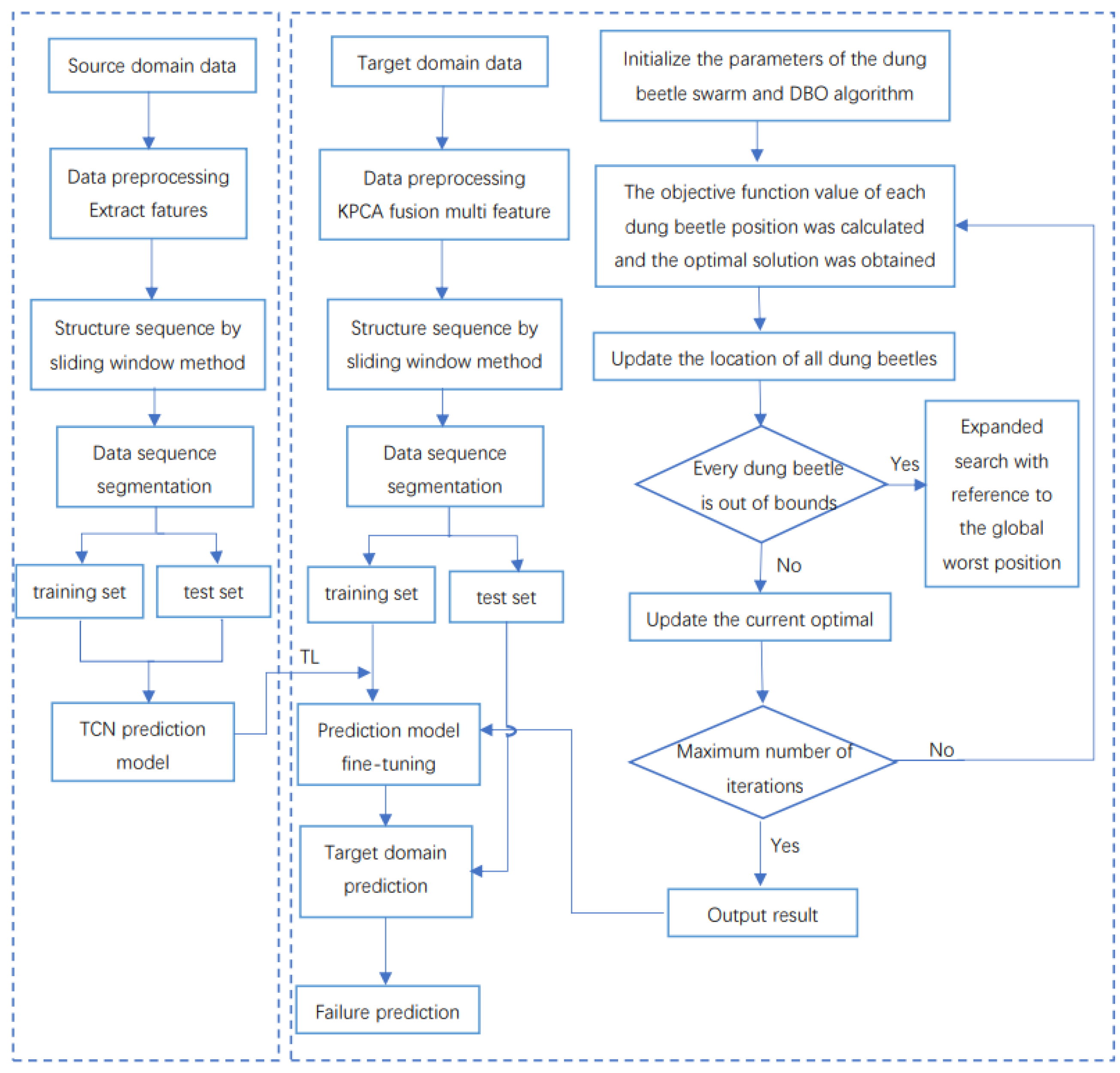
In this paper, a transfer learning method based on a TCN and the DBO algorithm is proposed to transfer the source condition with full life cycle degradation data to a new target condition for fault prediction. The flow chart of fault prediction using this method is shown in Figure 3.

3.1. TCN Modeling

The prediction model uses the TCN to extract the fault features in the signal. Since the data are one-dimensional time series data, and the one-dimensional convolutional layer in deep learning is mostly used for the feature extraction of time series data and text data, it is very suitable for the accelerated aging time series data of IGBTs in this paper.
The prediction method is as follows: Firstly, the decay parameters related to device performance are selected according to the requirements to form the training set and the test set. Secondly, the training set and test set are preprocessed to eliminate the influence of noise and dimension on the model’s prediction. Then, the model parameters are initialized, the optimizer is selected to train the training set iteratively, and the time backpropagation algorithm is used to adjust the model parameters. Finally, the test set is input into the trained TCN model, and the model output is the prediction data.
The time window method predicts the outcome at the next point in time based on data from that time period. The size of the time window determines how much data can be used to make the prediction. A smaller time window means that only a small amount of past data can be utilized, which may result in the model failing to capture complex patterns. A larger time window may contain too much data, making the model too complex to train and generalize. The studies in the current literature using the same IGBT dataset in the study selected a window length of 5 to construct the samples [20,21]. Therefore, in this paper, the sliding time window method was used to construct data samples with a window length of 5. That is, [[x0,x1,x2,x3,x4],[x5]] represents a time series sample constructed by the sliding window method. [x0,x1,x2,x3,x4] is taken as a sample and [x5] is taken as a sample label value, and so on, to obtain the input sequence and output sequence. The schematic diagram of the sliding time window method is shown in Figure 4.
The model uses the rectified linear unit (ReLU) function as the activation function after the convolutional layer because it has the advantages of simple derivation and sparsity of the activated data, which can reduce the network overfitting to some extent. The Adam optimizer was chosen because it can internally achieve dynamic adjustment of the learning rate convergence, thus improving the convergence speed and generalization ability of the model.

3.2. DBO Performance Testing

Currently, commonly used methods for parameter tuning include the particle swarm optimization (PSO) algorithm, whale optimization algorithm (WOA), dung beetle optimization algorithm, etc. PSO [22] has been applied in many fields. The principle is simple and easy to implement, but it lacks the dynamic adjustment of speed, and can easily fall into the local optimum, which will lead to low convergence accuracy and difficulty in converging. The WOA [23] has the ability to find the optimal solution in a shorter period of time with global search capability, but it is more dependent on the initial solution, and can easily fall into the local optimal solution. The DBO algorithm explores the search space thoroughly using information from different time periods and uses different update rules to ensure that the developed DBO algorithm maintains a sufficient balance between local and global search capabilities to avoid falling into the local optimum.
In order to test the optimization ability of the DBO algorithm, the DBO was compared with PSO and WOA. The two test functions were selected for simulation verification, in which the test function f 1 is a unimodal function and   f 2 is a multi-modal function. The specific test function expressions are shown in Table 1.
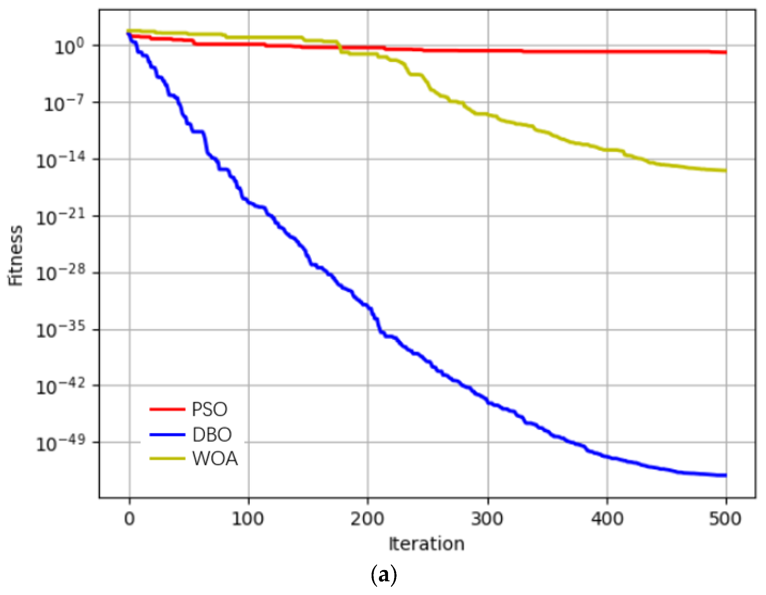
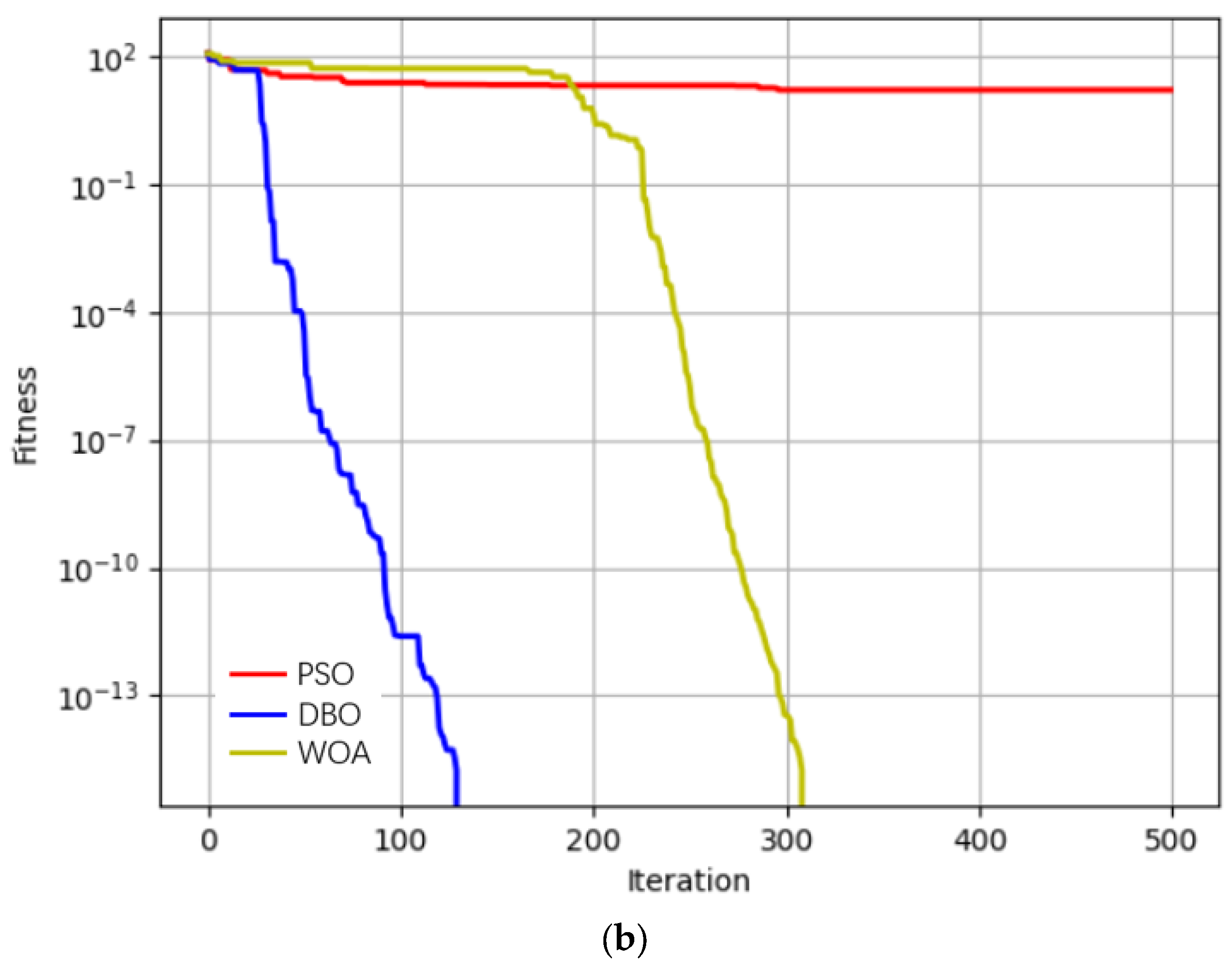
The population size of each algorithm was set to 30, the maximum number of iterations was 500, the dimension of the test function was 10, and each test function was run 20 times. The average fitness iteration convergence comparison curve of test functions f 1 and f 2 was drawn, as shown in Figure 5. The optimal value, standard deviation, and average value of the optimization results were calculated and analyzed. The comparison results of test functions are shown in Table 2.
From Figure 5, it can be seen that DBO has the least number of iterations among the three optimization algorithms with the same accuracy, and the convergence speed of the DBO algorithm is better than that of PSO and WOA.
From Table 2, it can be seen that when the test function is f 1 , although DBO, PSO, and WOA fail to find the optimal value, the DBO optimization result is closer to the optimal value, and then from the mean and standard deviation, the DBO algorithm performs better overall. When the test function is f 2 , both the DBO algorithm and WOA algorithm can find the optimal value with the same standard deviation, but from the mean value, DBO performs better. Therefore, it can be shown that among the three algorithms, the DBO algorithm has better stability, robustness, and superior performance in finding the optimal value.

3.3. DBO-TCN Optimized Transfer Learning Model

In this paper, the model transfer method was used to realize cross-case prediction, and its basic idea is as follows: The target domain is directly transplanted with the source domain network parameters in the establishment of the time series prediction model, and some of the TCN network parameters are fixed without changing. The data in the target domain are adjusted to another part of the network parameters that can be changed through network training so that the network is more suitable for the input–output mapping relationship in the target domain. Since the IGBT fault prediction problem studied in this paper belongs to the category of regression prediction, the three regression prediction index functions of mean square error (MSE), root mean square error (RMSE), and mean absolute error (MAE) were chosen to measure the performance of the model prediction algorithm, and their expressions are as follows:
M S E = 1 n i = 1 n ( y y ^ ) 2 R M S E = 1 n i = 1 n ( y y ^ ) 2 M A E = 1 n i = 1 n y y ^
where y represents the true value, y ^ represents the predicted value, n represents the number of predicted samples, and the smaller the value of the prediction indicator function, the better the network prediction performance.
From Section 3.2, it can be seen that the DBO algorithm has better stability and robustness and superior optimization performance, so in order to better adapt to the target domain, this paper adopts the DBO optimization method for the transfer model network parameter adjustment. The steps were as follows: Firstly, the TCN model trained in the source domain was frozen, and the obtained pre-trained model was used to initialize the model weights in the target domain. Secondly, the target domain was fine-tuned by using DBO for part of the network, and the multiple hyperparameters were iteratively optimized to improve the prediction accuracy and convergence speed of the model, so as to obtain an optimal combination of hyperparameters. Finally, the joint training of the unfrozen layer and the newly modified part was carried out on the target domain for the prediction.

4. Model Verification

For the IGBTs used in the rod control power supply cabinets of nuclear power plants, the devices are mainly controlled by applying the rectangular square wave voltage of pulse width in practice [24]. They have the same characteristics as the IGBTs used by the Prognostics Center of Excellence (PCoE) of National Aeronautics and Space Administration (NASA) for accelerated aging experiments on pre-drive power supply voltage and packaging method. For example, the pre-drive power supply voltage is 15 V, and the packaging mode is the welded type. The IGBT failure mode is closely related to the packaging mode of the power module. The main failure modes of welded IGBT power modules are bonding line failure and welding layer failure. Therefore, in the absence of the actual rod control power cabinet IGBT operation aging data, the IGBT accelerated aging dataset published by the PCoE was used to validate the research method proposed in this paper.
The environment used for validating the computational process was Python 3.9, and the computer configuration used for computation was an i5-8250U processor with 8 G RAM.

4.1. Data Presentation

The IGBT accelerated aging dataset published by the PCoE contains accelerated aging data for IGBTs under four experimental conditions, namely the experimental data of the source measurement unit (SMU) of the new equipment, accelerated thermal overstress aging with DC at the gate, accelerated thermal overstress aging with square signal at the gate, and accelerated thermal overstress aging with square signal at the gate and SMU [25]. The experimental verification work in this paper adopts the third and fourth types of experimental data for modeling. The experimental conditions of these two types of data are as follows:
(1)
Accelerated thermal overstress aging with a square signal at the gate. A square signal with a frequency of 10 kHz, a duty cycle of 40%, and an amplitude of 10 V was applied to the gate of the IRG4BC30K power device, and the temperature of the package was controlled to be 268–270 °C. In this case, the device was subjected to continuous overcurrent and a high-temperature aging test. The IGBT devices were continuously turned on and off, and the temperature of the package rose under the control of a drive mode with a fixed frequency and fixed pulse width. The driving mode with a fixed-frequency- and fixed-pulse-width control signal was turned off when the maximum temperature threshold was reached and was turned on again when the temperature was lower than the minimum temperature threshold. After 418 sets of the turn-on/turn-off test, the IGBTs latched up and the device failed. Each turn-on/turn-off set contained 100,000 collector–emitter voltage data.
(2)
Accelerated thermal overstress aging with a square signal at the gate and SMU. During the experiment, the emitter was connected to the ground wire of the power supply, and the collector and the resistor were connected in series to the positive lead of the power supply. The gate was driven by a high-speed amplifier that amplifies the output of a function generator to realize a jump in the device supply voltage from 2.5 V to 5.5 V with an amplitude of 0.5 V. A fixed-frequency- and fixed-pulse-width signal with a duty cycle of 40%, frequency of 1 kHz, and amplitude of 8 V was applied to the gate to control the opening of the IGBT device.

4.2. Data Pre-Processing

Taking the turn-on/turn-off data under accelerated thermal overstress aging with a square signal at the gate as an example, a transient voltage was generated during the turn-off of the IGBT due to the presence of parasitic components such as stray inductors, which, together with the turn-off voltage of the device produces the peak voltage shown in Figure 6. From the data comparison of groups 100, 200, 300, and 400 in the figure, it can be seen that the collector–emitter cut-off peak voltage values show a downward trend in the IGBT degradation process, and the peak voltage effect is very short, appearing at approximately 40,000–50,000 sampling points in each group. The horizontal coordinate of the figure represents the sequence number of sampling points, and the vertical coordinate represents the collector–emitter transient voltage value in V. This voltage will decrease with the degradation of the IGBT performance until the latch-up effect occurs, in which the relationship between the turn-off peak voltage and device degradation has been studied in the literature [25]. It is also proposed in the literature [26] that with the degradation of the IGBT performance, the turn-off peak voltage shows a decreasing tendency. Referring to the literature [25,26], the collector–emitter turn-off peak voltage was selected as the degradation parameter, which reflects the degradation law of IGBT performance.
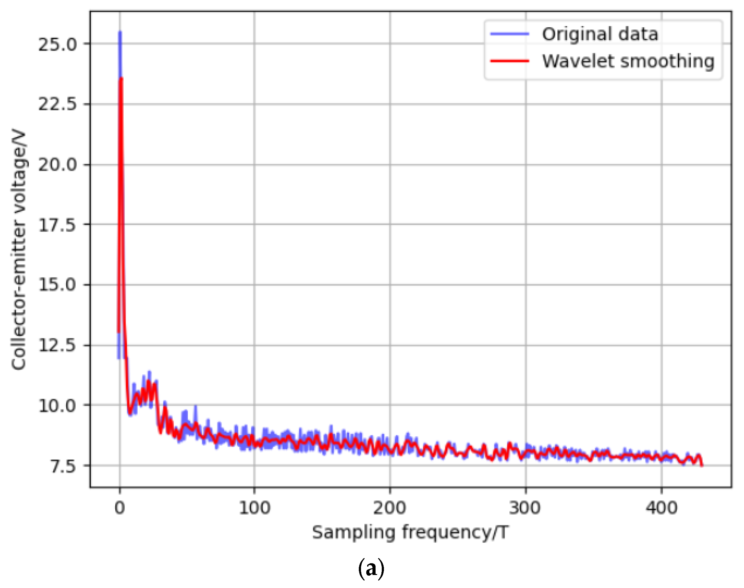
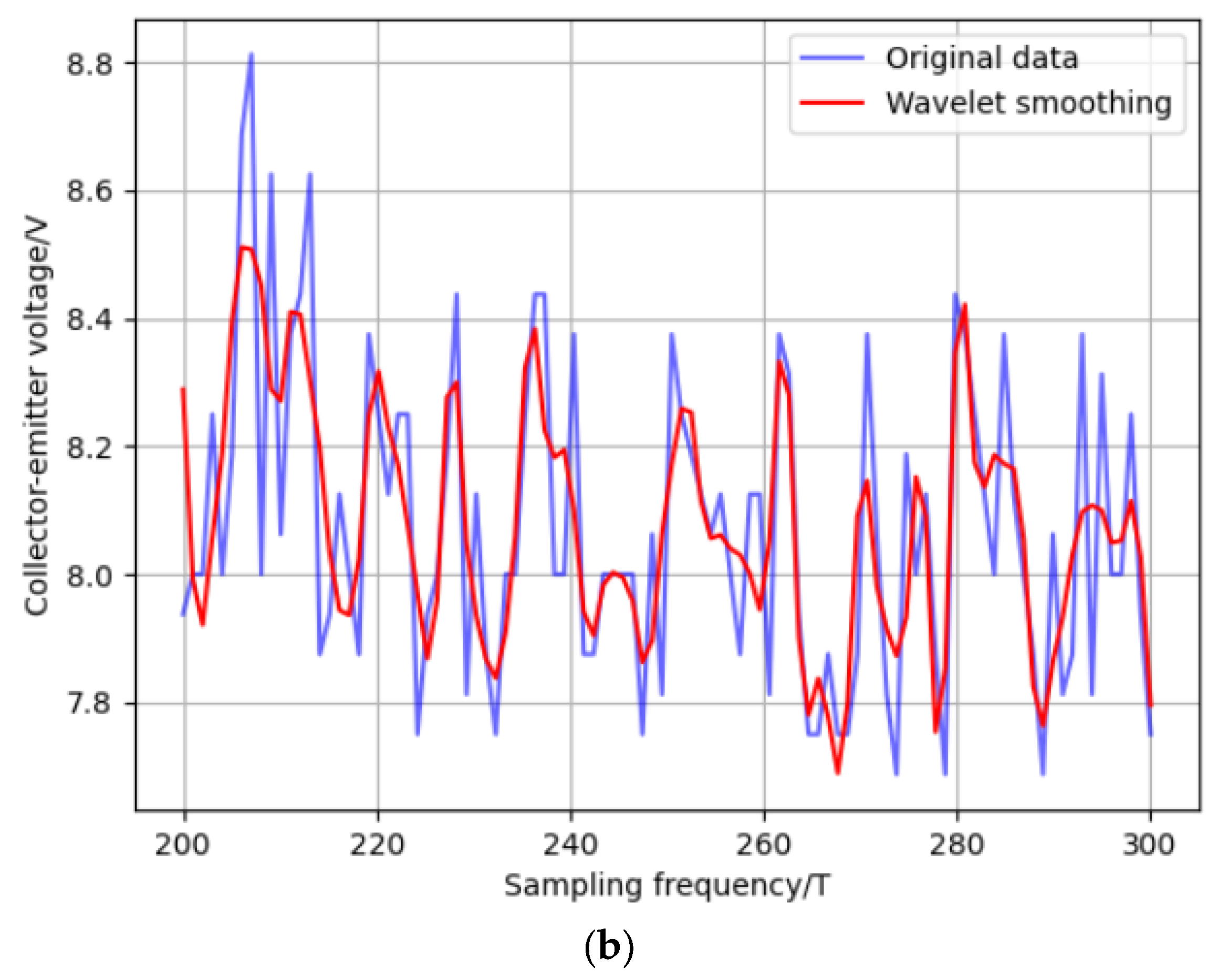
In the aging process of IGBTs, the peak voltage fluctuation is strong, but the general trend is downward; that is, with the aging of the device, the turn-off peak voltage becomes smaller and smaller. In this paper, wavelet transform was used to process the extracted turn-off peak voltage to reduce noise and sudden fluctuations and improve the accuracy of prediction. The comparison before and after signal processing is shown in Figure 7. It can be seen from the figure that compared with the original signal, the signal after noise reduction is smoother and retains the characteristics of the original signal better.
In order to reduce the influence of the network prediction results deviating from the actual values due to the different dimensions of the characteristic parameter samples, it is necessary to standardize the fault prediction values to improve the prediction accuracy, i.e.:
φ n = x n X M i n X M a x X M i n x n * = φ n M a x M i n + Min
where xn is the sample value; XMin and XMax are the minimum and maximum values of the sample; Min and Max are the specified minimum and maximum values; and xn* is the normalized value.

4.3. TCN-Based IGBT Fault Prediction Modeling

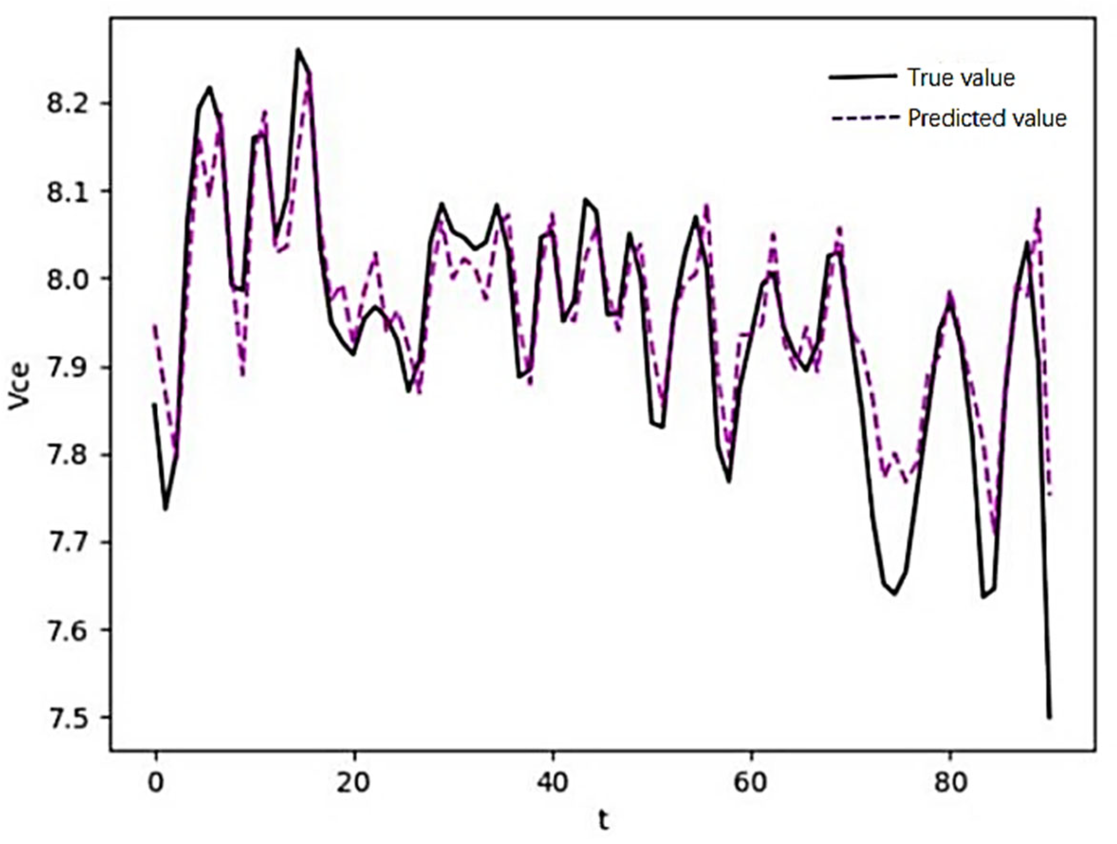
The TCN model proposed in this paper was verified by the experimental data of accelerated thermal overstress aging with a square signal at the gate. Firstly, the turn-off peak voltage of 418 groups of on–off data was extracted as the sample data, and the data were preprocessed by outlier removal, wavelet transform, standardization, etc. The preprocessed data were constructed as samples with a time window with a length of 5, 80% of the sample data were selected as the training set of the model, and 20% of the data were selected as the test set of the model. The model prediction results are shown in Figure 8.
From Figure 8, it can be seen that the TCN model accomplishes the prediction of IGBT recession parameters more effectively, and the predicted value curve roughly coincides with the target value curve. On the basis of the known initial turn-off peak voltage of the device, the failure can be predicted according to the model prediction curve by choosing a suitable threshold value in combination with the actual situation of the device. In order to further verify the superiority of the prediction method proposed in this paper, the LSTM, GRU, and RNN models were established according to the TCN modeling process, and the prediction results of these models were compared. The RNN is a classical sequence model that captures temporal dependencies in sequence data. The LSTM and GRU algorithms are commonly used as time series prediction algorithms because of their long-term memory capability and their ability to solve the problem of the long-range dependence of traditional recurrent neural networks. The mean square error, root mean square error, and mean absolute error were used as the indexes to evaluate the accuracy of model prediction, and the comparison results are shown in Table 3.
Table 3 shows that the model prediction accuracies of the TCN model are all better than those of the LSTM, GRU, and RNN models, proving that the TCN model is more accurate and effective for fault state trend prediction.

4.4. Optimal Transfer Learning Model of IGBT Based on DBO-TCN

The target domain selects the IGBT dataset under the experimental conditions of accelerated thermal overstress aging with a square signal at the gate and SMU. Since the power supply voltage, the maximum temperature threshold, and the minimum temperature threshold were not constant, in order to avoid using the amplitude as a single feature parameter and not fully reflecting the change trend of the signal in the experiment, six parameters were selected as eigenvalues to reflect the signal change process in the target domain. These parameters included the variance, standard deviation, skewness, kurtosis, barycenter frequency, and root mean square frequency of the time-domain waveform. The KPCA technique was used to integrate these six eigenvalues into one eigenvalue to characterize the degradation state of the IGBT, and the preprocessed data were used to construct the target domain samples with a time window with a length of 5. The specific transfer steps were as follows:
(1)
The TCN prediction model was obtained using the experimental data of accelerated thermal overstress aging with a square signal at the gate as the source domain.
(2)
Some network structure and weight parameters of the TCN model were frozen to keep them unchanged.
(3)
The DBO optimization algorithm was used to optimize the learning rate of the transfer model, the number of nodes in the hidden layer, and the number of training times, so as to obtain the parameters suitable for the samples in the target domain, and then the IGBT fault prediction model of transfer learning was obtained.
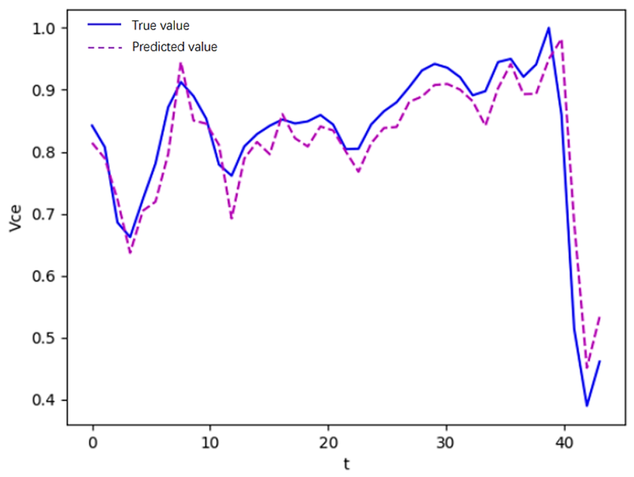
The prediction results of the model after transfer learning are shown in Figure 9.
From Figure 9, it can be seen that the transfer model better accomplishes the prediction of the IGBT recession parameters, and that the predicted value curve is closer to the true value curve. In order to further verify the superiority of the transfer learning model, the DBO-TCN model predictions after transfer learning were compared with the target-domain-retraining TCN model, LSTM transfer learning model, and GRU transfer learning model as shown in Table 4.
According to the prediction results in Table 4, the DBO-TCN transfer learning model shows great improvement in evaluation metrics compared to the target-domain-retraining TCN model, LSTM transfer learning model, GRU transfer learning model, and RNN transfer learning model. The DBO-TCN transfer learning model reduces the mean squared error, the root mean squared error, and the mean absolute error by 0.71%, 4.86%, and 4.45%, respectively, i.e., by a factor of two to three, compared to the target-domain-retraining TCN model. This indicates that the proposed method is more accurate and effective in predicting fault state trends. Moreover, in terms of model training time, the DBO-TCN transfer learning model requires less time compared to the retraining TCN model.

5. Conclusions

In this paper, an improved transfer learning prediction method based on a TCN is proposed to solve the problems of low efficiency and poor prediction results across the operating conditions of existing prediction methods. The method adopts the TCN method to predict the source domain data, which makes full use of the timing dependency relationship. The KPCA technique is used to fuse the time–frequency features of the target domain data into a feature indicator, which fully characterizes the IGBT degradation state and reduces the computational complexity. The DBO algorithm is used to optimize the number of hidden layers, the number of hidden layer nodes, and the learning rate of the transferred TCN prediction model, and the cross-condition prediction from the source domain to the target domain is realized. The results show that the transfer model method can significantly reduce the prediction error, which further confirms the excellent prediction performance of the model, and provides technical support for the fault prediction research of the IGBT in the rod control cabinet of a nuclear power plant.

Author Contributions

Conceptualization, Z.C. and L.Y.; methodology, L.Y.; software, L.Y.; validation, Z.C., L.Y. and Y.J.; formal analysis, Z.C.; investigation, L.Y.; resources, Z.C., L.Y. and J.L.; data curation, L.Y. and J.L.; writing—original draft preparation, L.Y.; writing—review and editing, L.Y., Z.C., J.L., C.L. and Y.J.; visualization, L.Y.; supervision, Z.C. and C.L.; project administration, Z.C. and L.Y.; funding acquisition, Z.C. and Y.J. All authors have read and agreed to the published version of the manuscript.

Funding

This research was funded by the National Natural Science Foundation of China, grant number [U2267206], and by the China National Atomic Energy Agency Stable Support Project, Project Name: Research on Intelligent Diagnosis and Health Management Technology for Key Electrical Drive Equipment in Nuclear Power Plants.

Data Availability Statement

The data presented in this study are available on request from the corresponding author. The data are not publicly available due to [protect the intellectual property rights of the authors’ affiliated institution].

Conflicts of Interest

The authors declare no conflicts of interest.

References

  1. Xu, Y.; Li, T.; Wang, C. Application of IGBT in rod control system of nuclear power plant. Autom. Instrum. 2014, 35, 41–43+46. [Google Scholar]
  2. Zhong, Z.; Wang, Y.; Huang, Y.; Xiao, D.; Xia, P.; Liu, C. Probabilistic sparse self-attention-based prediction of IGBT module remaining life across operating conditions. J. Shanghai Jiao Tong Univ. 2023, 57, 1005–1015. [Google Scholar]
  3. Alghassi, A.; Perinpanayagam, S.; Samie, M. Stochastic RUL Calculation Enhanced with TDNN-Based IGBT Failure Modeling. IEEE Trans. Reliab. 2016, 65, 558–573. [Google Scholar] [CrossRef]
  4. Oh, H.; Han, B.; McCluskey, P.; Han, C.; Youn, B.D. Physics of Failure, Condition Monitoring, and Prognostics of Insulated Gate Bipolar Transistor Modules: A Review. IEEE Trans. Power Electron. 2015, 30, 2413–2426. [Google Scholar] [CrossRef]
  5. Wu, Z.; Bai, H.; Yan, H.; Zhan, X.; Guo, C.; Jia, X. Intelligent Fault Diagnosis Method for Gearboxes Based on Deep Transfer Learning. Processes 2023, 11, 68. [Google Scholar] [CrossRef]
  6. He, B. Failure Mechanism Analysis of IGBT Based on Comsol Multiphysics Field Coupling Simulation; Harbin Institute of Technology: Harbin, China, 2021. [Google Scholar]
  7. Huang, K. Research on IGBT Module Performance Degradation and Fault Prediction Technology; Southwest Jiaotong University: Chengdu, China, 2022. [Google Scholar]
  8. Yuan, M.; Yin, Z.; Luo, P.; Zhang, Y. MPCC-based open-circuit fault diagnosis method for inverter IGBTs in permanent magnet synchronous motor drive systems. Electr. Drives 2023, 53, 25–31+54. [Google Scholar]
  9. Górecki, P.; Górecki, K.; Zarębski, J. Accurate Circuit-Level Modelling of IGBTs with Thermal Phenomena Taken into Account. Energies 2021, 14, 2372. [Google Scholar] [CrossRef]
  10. Held, M.; Jacob, P.; Nicoletti, G.; Scacco, P.; Poech, M.H. Fast Power Cycling Test for Insulated Gate Bipolar Transistor Modules in Traction Application. Int. J. Electron. 1999, 86, 1193–1204. [Google Scholar] [CrossRef]
  11. Bayerer, R.; Hermann, T.; Licht, T.; Lutz, J.; Feller, M. Model for Power Cycling Lifetime of IGBT Modules-Various Factors Influencing Lifetime. In Proceedings of the 5th International Conference on Integrated Power Electronics Systems, Nuremberg, Germany, 11–13 March 2008; pp. 1–6. [Google Scholar]
  12. Zhou, C.; Gao, B.; Yang, H.; Zhang, X.; Liu, J.; Li, L. Junction Temperature Prediction of Insulated Gate Bipolar Transistors in Wind Power Systems Based on an Improved Honey Badger Algorithm. Energies 2022, 15, 7366. [Google Scholar] [CrossRef]
  13. Zhou, A.; Mahemuti, P.; Li, G.; Zhao, Z.; Liu, H. Study on IGBT life prediction based on SMA-Elman. Microelectron. Comput. 2023, 40, 117–124. [Google Scholar]
  14. Ismail, A.; Saidi, L.; Sayadi, M.; Benbouzid, M. A New Data-Driven Approach for Power IGBTs Remaining Useful Life Estimation Based On Feature Reduction Technique and Neural Network. Electronics 2020, 9, 1571. [Google Scholar] [CrossRef]
  15. Bai, S.; Kolter, J.Z.; Koltun, V. An empirical evaluation of generic convolutional and recurrent networks for sequence modeling. arXiv 2018, arXiv:1803.01271. [Google Scholar]
  16. Gao, X.; Ma, D.; Han, H.; Gao, H. Fault prediction of complex industrial processes based on DAE and TCN. J. Instrum. 2021, 42, 140–151. [Google Scholar]
  17. Jin, S.; Si, F.; Dong, Y.; Ren, S. A Data-Driven Kernel Principal Component Analysis–Bagging–Gaussian Mixture Regression Framework for Pulverizer Soft Sensors Using Reduced Dimensions and Ensemble Learning. Energies 2023, 16, 6671. [Google Scholar] [CrossRef]
  18. Wang, J.; Chen, Y. Introduction to Transfer Learning, 2nd ed.; Electronic Industry Press: Beijing, China, 2022. [Google Scholar]
  19. Xue, J.; Bo, S. Dung beetle optimizer: A new meta-heuristic algorithm for global optimization. J. Supercomput. 2023, 79, 7305–7336. [Google Scholar] [CrossRef]
  20. Han, H. Research on IGBT Fault Prediction Based on Deep Learning; Beijing Jiaotong University: Beijing, China, 2019. [Google Scholar]
  21. Leng, L.; Fu, J.; Ning, B. Study on IGBT time series prediction based on SSA-LSTM model. Semicond. Technol. 2023, 48, 66–72. [Google Scholar]
  22. Deepak, M.; Rustum, R. Review of Latest Advances in Nature-Inspired Algorithms for Optimization of Activated Sludge Processes. Processes 2023, 11, 77. [Google Scholar] [CrossRef]
  23. Li, W.; Zhang, W.; Liu, B.; Guo, Y. The Situation Assessment of UAVs Based on an Improved Whale Optimization Bayesian Network Parameter-Learning Algorithm. Drones 2023, 7, 655. [Google Scholar] [CrossRef]
  24. Yang, P.; Zhang, J.; Wang, X.; He, Z.; Zheng, G. Simulation and optimization of nuclear reactor rod-controlled power supply circuit. Nucl. Technol. 2020, 43, 39–45. [Google Scholar]
  25. Zhang, M.; Wang, Q.; Yu, Y. IGBT fault prediction under thermal stress based on GRU and PCA-TL. Sci. Technol. Eng. 2023, 23, 4654–4659. [Google Scholar]
  26. Sonnenfeld, G.; Goebel, K.; Celaya, J.R. An agile accelerated aging, characterization and scenario simulation system for gate controlled power transistors. In Proceedings of the 2008 IEEE International Automatic Testing Conference, AUTOTESTCON, Salt Lake City, UT, USA, 8–11 September 2008; pp. 208–215. [Google Scholar]
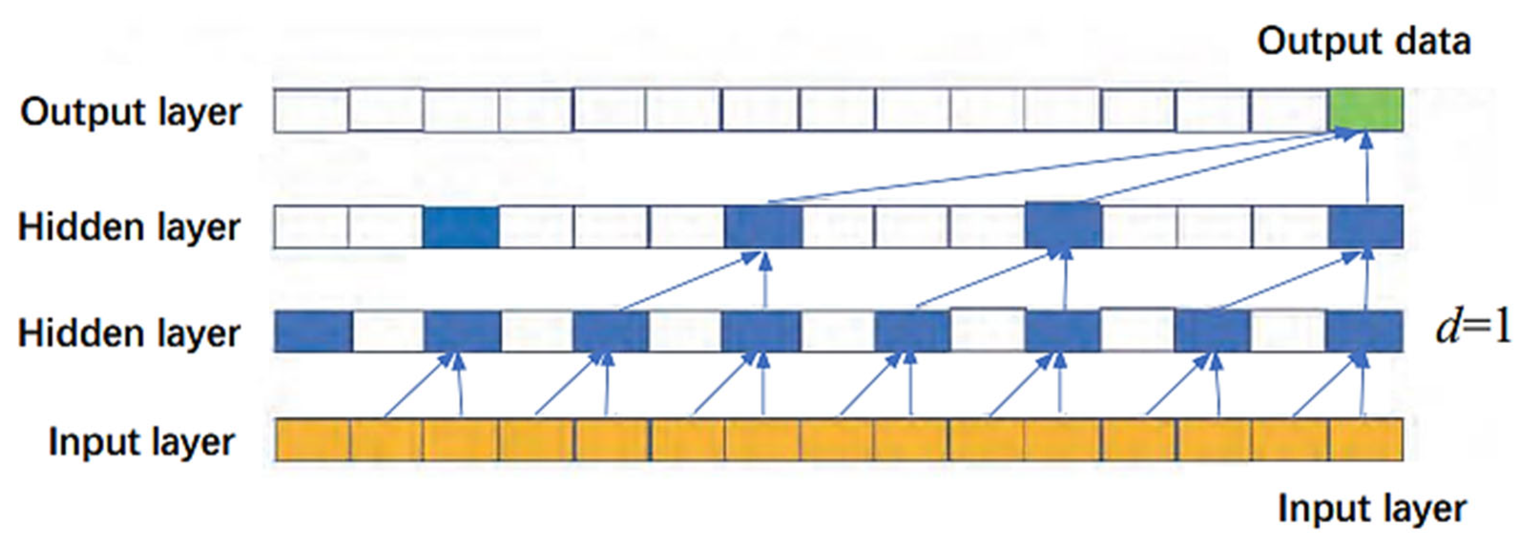
Figure 1. TCN convolutional structure.
Energies 17 00447 g001
Figure 2. Residual connection.
Energies 17 00447 g002
Figure 3. Fault prediction flow chart.
Energies 17 00447 g003
Figure 4. Sliding time window method.
Energies 17 00447 g004
Figure 5. Convergence curves of functions f1 and f2. (a) Convergence curve of function f1; (b) Convergence curve of function f2.
Energies 17 00447 g005aEnergies 17 00447 g005b
Figure 6. Shutdown peak voltage.
Energies 17 00447 g006
Figure 7. IGBT data noise reduction processing. (a) IGBT with all data noise reduction processing; (b) IGBT with part of the data noise reduction process.
Energies 17 00447 g007aEnergies 17 00447 g007b
Figure 8. TCN model prediction results.
Energies 17 00447 g008
Figure 9. DBO-TCN transfer model prediction results.
Energies 17 00447 g009
Table 1. Test functions.
FunctionSearch AreaOptimal Value
f 1 x = i = 1 D ( j = 1 i x i ) 2 [−100, 100]0
f 2 x = i = 1 D x i 2 10 cos 2 π x i + 10 [−5.12, 5.12]0
Table 2. Comparison results of DBO, PSO, and WOA in function test.
FunctionDBOPSOWOA
Optimal ValueStandard DeviationAverage ValueOptimal ValueStandard DeviationAverage ValueOptimal ValueStandard
Deviation
Average Value
f 1 7.81 × 10−548.50 × 10−283.19 × 10−291.28 × 10−12.07 × 10−1−9 × 10−33.29 × 10−161.05 × 10−84.77 × 10−10
f 2 05.56 × 10⁻¹⁰−5.90 × 10−111.61 × 1011.035−1.2 × 10−205.66 × 10−102.93 × 10⁻¹⁰
Table 3. Results of prediction model assessment indicators.
ModelMSE/%RMSE/%MAE/%
TCN0.366.054.7
LSTM2.1314.6211.16
GRU1.9413.9311.20
RNN2.5616.0212.01
Table 4. Comparison results of the transfer learning model and the target-domain-retraining TCN model.
ModelMSE/%RMSE/%MAE/%
DBO-TCN transfer learning model0.244.933.84
Target-domain-retraining TCN model0.959.798.29
LSTM transfer learning model2.2114.8811.15
GRU transfer learning model2.2515.0211.29
RNN transfer learning model3.0217.3912.97
Disclaimer/Publisher’s Note: The statements, opinions and data contained in all publications are solely those of the individual author(s) and contributor(s) and not of MDPI and/or the editor(s). MDPI and/or the editor(s) disclaim responsibility for any injury to people or property resulting from any ideas, methods, instructions or products referred to in the content.